en fr

HAL Id: tel-01404060

https://tel.archives-ouvertes.fr/tel-01404060

Submitted on 28 Nov 2016

HAL is a multi-disciplinary open access

archive for the deposit and dissemination of

sci-entific research documents, whether they are

pub-lished or not. The documents may come from

teaching and research institutions in France or

abroad, or from public or private research centers.

L’archive ouverte pluridisciplinaire HAL, est

destinée au dépôt et à la diffusion de documents

scientifiques de niveau recherche, publiés ou non,

émanant des établissements d’enseignement et de

recherche français ou étrangers, des laboratoires

publics ou privés.

Model Building by Temporal Logic Constraint Solving:

Investigation of the Coupling between the Cell Cycle

and the Circadian Clock

Pauline Traynard

To cite this version:

Pauline Traynard. Model Building by Temporal Logic Constraint Solving: Investigation of the

Cou-pling between the Cell Cycle and the Circadian Clock . Quantitative Methods [q-bio.QM]. Université

Paris Diderot, 2016. English. �tel-01404060�

T

HÈSE

présentée à

L’U

NIVERSITÉ

P

ARIS

D

IDEROT

(P

ARIS

7)

S

ORBONNE

P

ARIS

C

ITÉ

pour obtenir le titre de

Docteur

spécialité

Informatique

Model Building by

Temporal Logic Constraint Solving:

Investigation of the Coupling between

the Cell Cycle and the Circadian Clock

soutenue par

P

AULINE

T

RAYNARD

le 10 mai 2016

devant le jury composé de :

Président M. Ahmed BOUAJJANI

Rapporteurs M. Attila CSIKÁSZ-NAGY

M. Nir PITERMAN

Examinateurs Mme. Laurence CALZONE

Abstract

In this dissertation, we explore the use of temporal logic and model checking in systems biology. Our thesis is that temporal logic provides a powerful language to formalize complex yet imprecise dynamical properties of biological systems and to partly automate model building as a constraint satisfaction problem. We take advantage of this logical paradigm for systems biology to capture properties emerging from complex regulatory networks.

First, we investigate the ability of Computation Tree Logic to verify dynamical properties in asynchronous state transition graphs derived from logical models of the mammalian cell cycle. Logical modeling provides a qualitative and potentially non-deterministic description of a biological system. This feature is useful to account for a variety of dynamical properties, observed in different conditions within a generic model. We develop an approach of iterative property verification to assist the building and updating of logical models.

Then we consider quantitative deterministic models. For such models, oscillatory prop-erties such as pseudo-periods and pseudo-phases are formalized by quantitative constraints in First-Order Linear Time Logic. A continuous model can provide a precise description of the mechanisms governing a complex regulatory network, and a quantitative prediction of its dynamics. However, the classical difficulties associated with this approach are brought by numerous and often poorly characterized kinetic parameters. We address this challenge by im-plementing two complementary strategies to obtain efficient solving of dynamical constraints over a finite time horizon: the design of useful temporal logic formula patterns associated with dedicated constraint solvers, and some trace simplification rules to safely reduce the size of the traces to analyze.

We show that this approach enables the calibration of high-dimensional models on quanti-tative single-cell data with an application to model coupling for the mammalian cell cycle and the circadian clock. Understanding the relationships between these two molecular oscillators is an important problem in the field of chronobiology. We draw several coupling hypotheses and

Résumé

Cette dissertation explore l’utilisation de la logique temporelle et de la vérification de mod-èle en biologie des systèmes. Nous soutenons que la logique temporalle constitue un outil puis-sant pour formaliser des propriétés dynamiques à la fois complexes et imprécises permettant de caractériser un système biologique. Cet outil peut être utilisé pour partiellement automatiser la construction de modèle, comme une résolution d’un problème de satisfaction de contraintes. Tout d’abord, nous étudions l’emploi de la logique arborecente (Computation Tree Logic) pour vérifier des propriétés dynamiques dans des graphes de transitions d’états discrets asyn-chrones, dérivés de modèles logiques du cycle cellulaire mammifère. La modélisation logique fournit une description qualitative et potentiellement non-déterministe d’un système biologique. Elle offre un cadre utile pour rendre compte des diverses propriétés dynamiques observées dans différentes conditions au sein d’un modèle générique. Nous développons une approche de vérification itérative de propriétés pour assister la construction et la mise à jour de modèles logiques.

Puis, nous considérons des modèles quantitatifs déterministes. Pour de tels modèles, des propriétés sur les oscillations, telles que pseudo-période ou pseudo-phase, peuvent être for-malisées par des contraintes quantitatives en logique du premier ordre à temps linéaire (First-Order Linear Time Logic, FO-LTL). Un modèle continu peut fournir une description précise des mécanismes impliqués dans un réseau de régulations complexe, ainsi qu’une prédiction quan-titative de ses dynamiques. Cependant, une difficulté bien connue associée à cette approche provient du grand nombre de paramètres cinétiques, qui sont souvent mal caractérisés. Afin de répondre à ce problème, nous implémentons deux stratégies complémentaires pour améliorer l’efficacité de la résolution de contraintes dynamiques sur un horizon de temps fini. Une première approche exploite la définition d’une liste de motifs de logique temporelle fréquem-ment utilisés, associés à des solveurs de contraintes dédiés. Dans la deuxième approche, nous définissons et appliquons des règles de simplification de trace permettant de réduire la trace à analyser sans perte d’information.

Nous montrons que cette approche permet de calibrer des modèles de haute dimension sur des données quantitatives sur cellule individuelle. Elle est appliquée au couplage de modèles du cycle cellulaire et de l’horloge circadienne mammifères. Comprendre la relation entre ces deux rythmes moléculaires est un problème important dans le domaine de la chronobiologie. Nous déduisons différentes hypothèses de couplage et étudions leurs conséquences.

Remerciements

La thèse n’est pas un travail solitaire. Je dédie la mienne à celles et ceux qui par leur générosité, leur bonne humeur, par l’intérêt manifesté à l’égard de mon projet et leur implication, m’ont permis de progresser et d’aboutir dans cette phase de « l’apprenti-chercheur ».

Je tiens tout d’abord et spécifiquement à remercier Attila Csikász-Nagy et Nir Piterman pour avoir accepté d’être rapporteurs de ce mémoire, dont la version finale a grandement bénéficié de leur lecture attentive et de leurs précieuses observations. Je suis également reconnaissante à tous les membres du jury d’avoir accepté de se déplacer pour assister à la présentation de ce travail.

A François Fages et Denis Thieffry, mes directeurs de thèse, pour la confiance qu’il m’ont accordée en acceptant d’encadrer ce travail doctoral, pour m’avoir fait profiter de leurs connais-sances et bénéficier de leurs multiples conseils, pour le temps qu’ils ont consacré à diriger cette recherche, à relire et corriger tant nos articles que ce présent document, je veux exprimer mes plus chaleureux remerciements. Je leur suis également redevable des conditions de travail priv-ilégiées qu’ils m’ont apportées : entre l’IBENS et Inria, j’ai profité de deux environnements aussi riches que variés - partage qui m’a permis d’élargir mes horizons aussi bien en biologie qu’en informatique. Ils m’ont permis, à travers de multiples déplacements en conférences et en écoles d’été, de découvrir que le domaine de la recherche est un monde riche de personnes brillantes et accessibles, mues par la passion de la science, dont le dynamisme et le talent intellectuel forcent au respect et à l’humilité. Elles incarnent à merveille la devise affectionnée de François : « le plaisir de comprendre comme seule contrainte ».

Je ne veux pas oublier l’ensemble des deux équipes de recherche dont j’ai eu la chance de faire partie et mes collègues dans chaque institut : par les précieux moments partagés autour d’un thé, café, gâteau et autres pintes de bières, sans oublier les barbecues, cours de salsa et balades en raquettes, ils ont contribué à apporter une ambiance chaleureuse. Je remercie particulièrement la joyeuse équipe de sportifs d’Inria, notamment Victorien, Jonathan, Renaud, Sarah et Thierry. J’étais loin d’imaginer que cette préparation au doctorat ferait également de moi une fière candi-date au marathon. Nos entraînements assidus et bavards dans la riante forêt de Bailly seront de mes meilleurs souvenirs.

Au terme de ce parcours, mes pensées vont enfin à mes proches et amis qui - bien qu’un peu délaissés ces derniers mois - m’ont toujours adressé leurs encouragements. A mes parents va ma gratitude pour m’avoir offert le goût de la science, poussée à la curiosité intellectuelle, et donné toutes les chances pour réussir. Enfin une pensée pour Charles, pour son accompagnement et son réconfort, notamment durant les derniers mois de rédaction quand il partageait mes insomnies. A toi dont j’ai égoïstement saboté pas mal de soirées, week-ends et autres vacances, merci pour ton soutien indéfectible.

Contents

Contents 6

1 Introduction 8

1.1 Computational Systems Biology . . . 8

1.2 Abstraction of biological systems . . . 9

1.3 Model validation . . . 13

1.4 Outline . . . 17

2 Temporal constraints in the logical framework 18 2.1 Cell cycle . . . 18

2.2 Logical modeling framework . . . 19

2.3 Model analysis . . . 21

2.4 Application: studying the structural properties of the cell cycle . . . 24

2.5 Stochastic simulations of the logical model . . . 32

2.6 Conclusions and prospects . . . 34

3 Formalizing complex behaviors with temporal constraints 36 3.1 First Order Linear Time Logic for continuous trajectories . . . 36

3.2 Formalizing common properties for oscillatory systems with temporal logic . . . . 43

3.3 Illustration: parameter analysis of a toy oscillator model . . . 50

3.4 Conclusion . . . 57

4 _{Efficient solving of FO-LTL(Rlin) constraints} 58 4.1 Solving complexity . . . 58

4.2 Dedicated solvers for complex specifications . . . 59

4.3 Trace simplification preserving temporal specifications . . . 73

4.4 Trace simplification for selecting main peaks . . . 80

4.5 Conclusion . . . 84

5 Application to the coupling between the cell cycle and the circadian clock 86 5.1 Introduction . . . 86

5.2 Experimental data and their formal specification in temporal logic . . . 89

5.3 Cell Cycle and Circadian Clock Models . . . 92

5.4 Coupled Model . . . 96 5.5 Alternative hypotheses . . . 103 5.6 Bidirectional coupling . . . 108 5.7 Conclusion . . . 110 6 Conclusion, prospects 112 6.1 Summary . . . 112 6.2 Contributions . . . 113 6.3 Prospects . . . 114

Contents

Bibliography 116

A Appendix 127

A.1 Perturbation properties and CTL formulae for the logical model of the cell cycle . . 127 A.2 Toy oscillator model . . . 130 A.3 Models studied in Chapter 5 . . . 130

1.

Introduction

“

François Jacob, 1974

”

1.1

Computational Systems Biology

Systems approach for biology

Molecular systems biology: from molecules to processes

Describing biological processes with mathematics is a challenge of increasing importance in mod-ern biology. On the molecular level, biochemical reactions form intra- and intercellular relation-ships between molecular components and delineate networks of interconnected and mutually dependent molecules.

The study of regulatory networks relies on a systems approach, formalized with computa-tional models. This approach explains the paradoxical tolerance of huge variability of behaviors observed among similar organisms, organs and cells: inherently stochastic individual trajecto-ries are constrained in robust biological systems. Feedback-based constraints cause high-level behaviors to emerge and are responsible for maintaining the stability of global properties.

The approach of building explanatory and predictive computational models from the bio-chemical elements of living organisms is central in the field of systems biology. The goal of this extensively multidisciplinary research field, fed with techniques borrowed from other disciplines such as non-linear dynamics, statistics, control theory, graph theory, was described by Kitano in 1999: "Gain system-level understanding of multi-scale biological processes in terms of their elementary interactions at the molecular level." Proposing a model accounting for the observed cell responses, or better, predicting novel behaviors, is now regarded as an essential step to validate a proposed mechanism in systems biology.

Cells as complex biochemical integrative circuits

The development of systems biology is fueled with the constant improvement of experimental tools, resulting in informative data on biological systems responses in various environmental and stimulation conditions and at different scales, from single cell to whole organism. At the molec-ular level in particmolec-ular, the increasingly precise knowledge of interactions composing molecmolec-ular networks and their mechanisms derives from the huge amount of biological data generated by high-throughput methods and analyzed by functional genomics. A high variety characterizes these mechanisms: chemical reaction, complex formation, binding, transcriptional regulation, etc.

1.2. Abstraction of biological systems Abstracting molecules as functional elements that execute operations on a signal helps reducing the complexity.

From this point of view, cells can be seen as biochemical integrative circuits in which com-plex regulatory networks integrate and process information from multiple external signals, and compute an adequate answer. Accumulation and optimization driven by evolution make them efficient, robust and flexible. The approach of describing biological systems as executable models is detailed in particular in [Fisher and Henzinger, 2007]. The difficulties of understanding such circuits lie in part in the number of molecular species and their interactions, but most of all in the nature of the biochemical computation, which is high dimensional, concurrent, distributed and stochastic, and relies on tight controls to enforce specific cellular responses. In particular, biological processes operate at widely disparate time and spatial scales and commonly involve nonlinearities. Hence, processing biochemical information requires an understanding of control notions such as structural stability, resilience, and robustness.

It creates a strong push for the development of methods that analyze large interaction net-works and produce quantitative predictions that match single cell data precision and robustness, and multiscale models that take into account biological variability and population effects. Dedi-cated mathematical and computational approaches are needed to calibrate models to experimen-tal data.

Formal methods for systems biology

Computational Science, as the field of study concerned with the theoretical foundations of in-formation and computation, brings useful techniques to the modeling and understanding of molecular biological networks. Beyond the algorithm and computing power, able to deal with the high number of behaviors produced by combinatorial composition and stochastic trajecto-ries, and the definition of common standards and methods that structure the systems biology community (such as repositories for data, ontology or biological models), the most important contribution is a wealth of formal methods borrowed from programming theory and designed to deal with complex networks. These methods are increasingly used for the formal analysis of natural processes such as biological behaviors.

Formal methods rely on abstraction to infer properties from complex systems. In particular, methods for the systematic study of the structure, correctness and efficiency of computational systems are adaptable to biological systems.

1.2

Abstraction of biological systems

Model building

Understanding the temporal behavior of biological regulatory networks requires the integration of regulatory data into a formal dynamical model. This abstract representation of a biological system fulfills several essential roles:

• to formalize existing knowledge,

• to bring understanding of dynamical features of biological networks, • to make predictions on the system,

• to assist the rational design of novel informative experiments.

These roles fall within contradictory perspectives. On the one hand, knowledge representa-tion implies to take into account all known interacrepresenta-tions with the maximum of details. However, some relations between molecules sometimes need to be abstracted for lack of knowledge of

1. INTRODUCTION

necessitates heavy abstractions. In general, models for making predictions should represent the minimum information sufficient for answering particular questions, in order to maximize the efficiency of available tools. This classic difficulty faced by modeling is highlighted by Olaf Wolkenhauer [Wolkenhauer, 2014]: "The model should be as simple as possible and as detailed as necessary. [...] Thus modeling is the art of making reasonable assumptions and appropriate choices." The same trade-off appears for program analysis and is at the heart of the theory of abstract interpretation [Cousot and Cousot, 1977, Fages and Soliman, 2008]. Therefore each decision has to be made with the objective of a good balance between computational cost and precision of the dynamics. For example, considering gene regulation, the activation of a gene may be modeled by taking into account the different processes from transcription to translation, or by simply considering that the gene is activated. Most of all, a model has to be built adequately to address specific questions.

These objectives are best achieved through an iterative modeling process, ideally forming a cy-cle of data-driven modeling and model-driven experimentation, as shown in Figure 1.1. Phases of model building, refinement or extension, are interwoven with phases of model validation, where experiments performed on the model allow to verify relevant properties and assess whether the model achieves a useful approximation of the system. A negative outcome reveals the need of changes in the model and give new insights into the underlying mechanisms. Many choices have to be made along this process, starting with the level of precision of the initial model, to the formalism and abstraction used to describe the dynamics, the properties to check, and the successive refinements needed to reach a satisfactory description of the system.

Computational model Hypothesis Validation Dry experiment Wet experiment New data Biological

phenomenon Experimental data

validated invalidated Predictions Wet experiment New data

Figure 1.1: The cycle of model building: a computational model is built on experimental data on the basis of hypotheses accounting for missing data or unobserved conditions. These hypotheses have to be validated with well-chosen experiments that generate new data, which are integrated in the model and lead to modifications. If the model is invalidated, the model has to be revised with different hypotheses, potentially with the help of new data.

Hierarchy of semantics

Whatever the chosen level of precision, abstracting a biological system in a formalized model is done in several steps. It starts with a regulatory map that integrates and organizes the knowledge on the system. Tools like CellDesigner [Funahashi et al., 2008] facilitate the construction and maintenance of large or detailed maps. The map is then abstracted into an influence graph con-stituting the model structure with chosen components and describing the relationships between

1.2. Abstraction of biological systems modeled quantities. Finally, the influence graph is formalized in a model with a chosen semantics, depending on the amount of dynamical parameters that can be estimated, the available data and the expected result [Franke et al., 2010].

Different semantics have been developed to formalize biological systems, and can be classified in two main categories: quantitative and qualitative. The most frequently used semantics are introduced below.

• Logical models (qualitative)

If precise mechanisms for interactions are unknown and the data about the system’s behav-ior is mostly qualitative, the influence graph can be directly used to build a logical model. This qualitative approach based on Boolean algebra or generalization thereof [Glass and Kauffman, 1973, Thomas, 1991] offers a flexible framework to delineate the main dynamical properties of complex biological regulatory networks. In this formalism, the activity levels of regulatory components are abstracted into discrete variables and their dynamics are represented by transitions between discrete states of the system (see [Chaouiya and Remy, 2013] for more detail). The time is implicitly represented through the discrete transitions. The logical framework has been used successfully to construct and analyze large networks [Albert and Thakar, 2014, Naldi et al., 2015, Le Novere, 2015].

• Continuous models (quantitative)

Quantitative models are essentially based on systems of ordinary differential equations (ODEs), representing the continuous evolution of each molecule concentration, with a con-tinuous time. This formalism provides quantitative predictions, and dynamical systems analyses techniques such as phase portrait and bifurcation analysis can be used to study the possible dynamics (used for example in [Leloup and Goldbeter, 2003, Csikász-Nagy et al., 2006, Novák and Tyson, 2008]). Since kinetic parameters have to be calibrated with experimental data, this formalism suffers from the lack of reliable kinetic data for the regula-tory mechanisms and the high levels of noise in experimental data. Analyzing a continuous model is based on deterministic numerical simulations, which offers a partial view of the system dynamics properties, restricted to a particular set of parameter values. Moreover, detailed simulations are computationally expensive and often result in time consuming analyses. In Figure 1.2, a simple reaction of repressed mRNA transcription is represented as a regulatory map, and modeled with logical and continuous semantics.

• Stochastic models

Attempts at modeling intrinsic and extrinsic noise have increased the interest in stochastic methods. Logical and continuous semantics can be extended to include stochastic rates, in order to take into account the high variation exhibited by some processes that involve a small number of molecules, such as transcription. For example, stochastic equations are a refinement from differential models that includes additional stochastic variables repre-senting uncertainty in parameters, reaction rates, or network structure. When biological variability as well as uncertainty in measurements may significantly affect the interpretation of data, stochastic models relying on Markov processes and simulated with Continuous Time Markov Chains (CTMCs) are better suited, at the cost of a heavier computational effort [Wilkinson, 2009]. The compositionality offered by process algebra, originally developed for describing computer processes, is also a successful approach to model biological systems as concurrent systems [Regev et al., 2001].

In this dissertation we focus on non-stochastic logical and continuous modeling. While this choice impacts greatly on the dynamical results, theorems allow to draw conclusions from one semantic to another one. Although it overtakes the scope of this thesis, it is important to have in mind that links can be drawn between different modeling semantics, and that most analysis techniques can be adapted from one semantic to another.

Some formalisms support various semantics with extensions. For example, Petri nets are a graphical and mathematical formalism suitable for the modeling and the analysis of concurrent,

1. INTRODUCTION R mRNA 00 11 01 10 R mRNA 0 1 0 1

Figure 1.2: Left: CellDesigner-style regulatory map of a repressed mRNA transcription. Middle: Logical modeling of a repressed mRNA transcription with two Boolean components R (repressor) and mRNA. The dynamics on the bottom exhibits two stable states (round nodes): mRNA is active if R is inactive, and mRNA is inactive if R is active. Right: ODE modeling a repressed mRNA transcription with a Hill function. R is the repressor concentration, k1 is the maximal expression rate when there is no repressor, Km is the repression coefficient, equal to the concentration of repressor needed to repressed by 50% the overall expression, and n is the Hill Coefficient. It controls the steepness of the switch between no-repression to full-repression. On the bottom, the level of transcribed mRNA versus R is displayed.

logical systems, based on the number of molecules for each species and simulated with multiset rewriting [Reddy et al., 1996, Chaouiya, 2007]. However, extensions of the formalism allow the consideration of stochastic or continuous models.

Based on the theory of abstract interpretation, links can be drawn between different semantics. In [Fages and Soliman, 2008], Galois connections have been shown to link in the logical formalism the syntactical, stochastic, discrete Petri Net and Boolean semantics. Moreover, for ample con-ditions the ODE semantics approximates the mean stochastic behavior [Gillespie, 1977]. These abstraction relationships are summarized in Figure 1.3.

Developing common formalisms for different semantics, and relationships between semantics is useful to draw links between models. Techniques of model reduction [Naldi et al., 2011, Naldi et al., 2012], modular modelling (see for example [Fauré et al., 2009]) or hybrid [Lincoln and Tiwari, 2004, Chiang et al., 2015] and multiscale modeling can then take advantage of exist-ing models to broaden the analysis of already studied biological systems at multiple levels of organization (gene, protein/enzyme, cell, tissue, organ, organism). Population models can be approximated by stochastic models that use ODEs modelling higher order moments to estimate the mean and variance. Proper population models, based on PDEs and agent-based simulations (for example in [Billy et al., 2014]), usually capture less details on the molecular machinery of the cell, but account for cell-to-cell variability. Multiscale models attempt to describe both molecular interactions and population characteristics such as growth rate [El Cheikh et al., 2014].

1.3. Model validation concrete Stochastic CTMC Petri Nets abstract Boolean Syntactical Continuous ODE

Figure 1.3: Hierarchy of semantics described in [Fages and Soliman, 2008]: Boolean semantics can be abstracted from logical semantics, which can be abstracted from stochastic semantics based on Continuous-Time Markov Chains. Continuous semantics based on ODEs abstracts the mean behavior of stochastic semantics in some conditions.

1.3

Model validation

Formal specifications of dynamical behaviors

A model is validated relatively to a considered behavior by checking the coherence of its dy-namics with available data on this behavior. Different in silico experiments can be used to infer dynamic properties that will be most relevant to confront with the data, which can be quantitative or qualitative, incomplete or uncertain, reflect different conditions of perturbations of the system, and may need a phase of preprocessing.

Asymptotic properties can usually be determined with static analysis methods based on struc-tural conditions rather than simulations. For example, steady-state analysis finds equilibrium states of the systems on topology grounds. On the other hand, formalizing properties on the tra-jectories of the system is more complex, because of the wide possibility of possible behaviors. Of crucial importance is the selection and correct specification of relevant properties. For example, comparing a simulation trajectory to an experimental trace with a general comparison method such as curve-fitting poses great risks of over-specification in case of imprecise or noisy data.

This problem is addressed by the formalization of complex properties with temporal logic, a formal system for representing and reasoning about propositions qualified by the orders of events in time. Properties expressed in temporal logic are automatically verified against a model by model checkers. In this dissertation, we explore the use of temporal logic to formalize complex yet imprecise dynamical properties of biological systems for different semantics, and to partly automate model building as a constraint satisfaction problem.

Model checking

Model checking is a computer science technique that aims at determining whether a dynamical system, formalized as a finite-state automaton, satisfies a set of properties, themselves formalized as logical specifications. It has been initially proposed in the 1980s to reason about very large hardware and software systems, typically to check for the absence of deadlock and critical state

1. INTRODUCTION

intractable. This motivates the use of automated formal verification techniques that explore exhaustively and automatically finite models of programs so as to determine whether undesirable error states are accessible.

The system dynamics is formalized as a Kripke structure, which is an oriented graph repre-senting the transitions between the different states of the system. Each path in the graph, starting from some initial states, represents a sequence of states separated by permissible transitions, i.e. a possible computation of the system. Model-checkers use specific algorithms to verify properties in the graph.

The size of the model is critical for the checking phase to be practical. Traditional model check-ing is based on Binary Decision Diagrams and is implemented in symbolic model checkers such as NuSMV [Cavada et al., 2002]. This approach has been complemented by various successful model checking algorithms based on SAT-solving, such as IC3 [Bradley, 2011]. In the frame of biological systems viewed as programs, it is natural to use model checking tools to verify the validity of biological properties in a system. In this respect, in mid 2000s, model checking started to be applied in the broad field of Systems Biology, mainly for the verification of qualitative systems dynamics. Successful applications include [Chabrier-Rivier et al., 2004, Bernot et al., 2004, Batt et al., 2005, Gong et al., 2011].

This approach makes a bridge between theoretical models and biological experiments, through the following identifications:

biological model = transition system, biological property = temporal logic formula,

model validation = model checking, model inference = constraint solving.

Initially developed for discrete systems, model checking methodologies have been improved, as well as their range of applicability, and the tools have been extended to deal with real-time and limited forms of hybrid systems. Temporal logic specifications are applied differently on logical models and continuous models, although the challenge is the same: automatically decide if the dynamics of the model satisfies a given temporal property. On the one hand, the simplicity of the logical framework allows the logical symbolic verification of qualitative temporal logic specifications for all possible dynamics of the model with model checking methods. On the other hand, extensions of temporal model checking techniques enable quantitative verifications with continuous semantics, such as robustness. But the verification relies on numerical simulation and is restricted to a given parameterization.

Formalizing dynamical behaviors with temporal logic

Different temporal logics exist, each with specific operators to reason about time. The most widely used are the Linear Time Logic (LTL) and the Computation Tree Logic (CTL), which have been developed successively and have become standards in the model checking community. All properties expressible in either logic can also be expressed in the superset CTL*.

Computation Tree Logic (CTL)

CTL is a branching-time logic that can reason about multiple time lines [Clarke et al., 1999] organized in a tree-like structure, and is thus adapted to non-deterministic automata derived from discrete models. Symbolic methods avoid enumerating each state of an automaton, which can be costly, by representing sets of states and transitions. A widely adopted method uses binary decision diagrams (BDDs). Another method called Bounded Model Checking (BMC) [Clarke et al., 2001] uses a propositional SAT solver rather than BDD manipulation techniques and looks for solutions of size smaller than a user-provided bound. Extensions of CTL exist, for example the Action Restricted Computation Tree Logic (ARCTL) [Monteiro and Chaouiya, 2012] is used to account for a distinct semantics of inputs and internal (regulated) components. It imposes an additional path restriction on a subset of inputs while letting others inputs to freely vary.

1.3. Model validation

Linear Temporal Logic (LTL)

LTL is restricted to reasoning about one time line, and can thus be successfully used to charac-terize deterministic dynamics. Otherwise, it checks the satisfaction of a property successively on all possible sequences of states. Similarly to CTL, solving LTL specifications can be done with BDDs or SAT solvers in the BMC framework. Initially applied to discrete systems, LTL can be generalized to quantitative models in two ways: either by discretizing the different regimes of the dynamics in piece-wise linear or affine models [de Jong et al., 2004, Batt et al., 2010], or by relying on numerical simulations instead of symbolic solving and taking a first-order version of temporal logic (FO-LTL) with constraints on concentrations, as query language for the numerical traces [Fages and Rizk, 2008]. Such language can be used not only to extract information from numerical traces coming from either experimental data or model simulations, but also to specify the expected behaviors as constraints for model calibration and robustness measure [Rizk et al., 2009, Rizk et al., 2011, Donzé et al., 2013].

Other extensions of temporal logics have been developed for quantitative model checking, like the continuous interpretation of Signal Temporal Logic [Donzé and Maler, 2010], which has been successfully used in [Stoma et al., 2013] to build a model of TRAIL-induced apoptosis and revisit the classification of T-cells, or for oscillation constraints in [Banks et al., 2015]. However, STL is limited by the inability to distinguish signal values occurring in time points in which some local property is satisfied. In [Brim et al., 2014], an extension of STL logic denoted STL* based on a signal-value freeze quantification allows referencing a signal value in a time point. In this formalism, suited for nontrivial real-time processes, a property satisfaction problem is solved with an approximate monitoring procedure. The grammar uses bounded operators constrained by time intervals.

FO-LTL, in contrast, is suited for smooth signals supporting derivatives and uses unbounded operators, which allows the definition of complex specifications on a whole trace.

Thesis

The formalization of biological properties as a specification in temporal logic remains a delicate task and a bottleneck of this approach.

In this dissertation, we explore the use of both CTL and FO-LTL for constraint solving in systems biology. Although both have already been used in various studies, we investigate their application to analyze oscillatory systems, which necessitate to formalize more complex behav-iors than previously done.

For example, in [Batt et al., 2005] CTL specifications have been used with model-checking methods to test conditions leading to a given state in a model, imposing restrictions on sequences of events along the path.

Moreover, the method based on FO-LTL and described in Chapter 3 has been used in cell signaling to elucidate the complex dynamics of GPCR signaling in [Heitzler et al., 2012]. How-ever, the specifications defined in this study were mostly based on curve-fitting, a technique that requires precise quantitative and temporal data. In that case, some response curves in a model of GPCR signaling were available, and the failure to fit them was the key to revisit the structure of GPCR signaling interactions, and propose a different mechanism that has been verified experimentally. As another example, a temporal logic specification of timing constraints in a model of a genetic switch was successfully used in [Rizk et al., 2009] to compute global sensitivity indices and improve the design of a synthetic switch.

We investigate the definition of temporal logic specifications that are more complex than curve-fitting or simple reachability. Our work highlights the ability of this formal framework to specify a wide variety of dynamical behaviors, and to deal with imprecise data. For example, as will be detailed in Chapter 3, FO-LTL allows us to combine qualitative properties of oscillations and quantitative properties on the shapes of the traces such as distances between peaks or peak amplitudes. This is useful to capture the periods on both experimental and simulated traces, even

1. INTRODUCTION

Constraints for model synthesis: parameter inference

Calibrating dynamical models on experimental data is a central task in computational systems biology. Beyond property verification, the logical paradigm exposed earlier allows to develop methods of model synthesis as constraint solving problems. Given a regulatory network, the goal is to infer a parameterization (logical or continuous rules) that satisfies a list of properties specified as constraints.

When logical or numerical values for model parameters can be found to fit the data, the model can be used to make predictions, whereas the absence of any good fit may suggest to revisit the structure of the model and gain new insights in the biology of the system, see for instance [Stoma et al., 2013, Heitzler et al., 2012]. The validation of the model is thus a phase of intelligent assistance for the design of new experiments.

In particular, several optimization methods have been developed to infer kinetic parameters for continuous models by fitting timed quantitative data such as time series. They are increasingly used as technical innovations in experimental devices now produce precise temporal data with single-molecule measurements and single-cell time series.

The difficulty for model calibration is to identify the most relevant characteristics from the quantitative data and avoid over-fitting. Temporal logic provides a generic method to specify dynamical behaviors wile combining expressiveness and flexibility.

Complexity

The general idea of model-checking a single finite trace has been well known for years, notably in the framework of Runtime Verification [Markey and Schnoebelen, 2003]. It usually relies on the classical bottom-up algorithm, which is bilinear [Ro¸su and Havelund, 2005]. This extends even to quantitative model checking like the continuous interpretation of Signal Temporal Logic [Donzé and Maler, 2010] since the combination of two booleans or two reals by min/max is cheap. However, when using the full power of First-Order Linear Time Logic (FO-LTL) to compute validity domains, the dependency of the complexity on the size of the trace is no longer linear but exponential in the number of variables [Fages and Rizk, 2008], reflecting the computational cost of combining complex domains. In this dissertation we address this issue with two approaches to improve the performance of FO-LTL constraint solving, and with it of the corresponding calibration methods: a trace simplification procedure prior to the constraint solving [Traynard et al., 2014] and the definition of dedicated solvers for frequently used properties [Fages and Traynard, 2014].

Modelling platforms

Two modelling softwares have been mainly used for the work presented in this thesis: GINsim for logical modelling and Biocham for continuous modelling.

• GINsim - http://ginsim.org

The logical model presented in Chapter 2 has been built and partly analyzed with GINsim. This software suite has been developed to facilitate the definition, the simulation, and the dynamical analysis of logical models [Naldi et al., 2009, Chaouiya et al., 2012]. In particular, this software supports STG construction for different updating assumptions. In addition, it provides a function to compress state transition graphs by regrouping the states into compo-nents leading to the same attractors or cyclic compocompo-nents, thereby easing the identification of dynamical attractors (stable states, simple or complex cycles) along with their basins of attractions [Bérenguier et al., 2013]. Finally, GINsim enables the definition and storage of different initial states and perturbations (e.g. gain- or loss-of-function mutants).

• Biocham - http://lifeware.inria.fr/biocham The logical paradigm for systems biology is at the heart of the development of the biochemical abstract machine (BIOCHAM) modeling

1.4. Outline platform [Fages, 2005, Calzone et al., 2006]. Over the last decade, this software environ-ment has been developed to model cell biology molecular reaction systems, reason about them at different levels of abstraction, and formalize biological behaviors in temporal logic with numerical constraints. Biocham allows us to analyze dynamical properties, infer non-measurable kinetic parameter values, and evaluate robustness.

Several methods for efficient solving of temporal specifications, in particular trace simplifi-cation [Traynard et al., 2014] and dedicated solvers [Fages and Traynard, 2014], have been developed as part of this work and implemented in Biocham.

The continuous model presented in Chapter 5 has been built using the BIOCHAM modeling software for

1. importing and exporting models in SBML, and modeling the molecular interactions of the coupling of the models,

2. specifying experimentally observed behaviors in quantitative temporal logic using relations for periods and phases [Fages and Traynard, 2014, Traynard et al., 2014], 3. searching parameter values [Rizk et al., 2011] and measuring robustness and

parame-ter sensitivity indices [Rizk et al., 2009] with respect to the temporal logic specification of the dynamical behavior,

4. making biological hypotheses on the coupling between the cell cycle and the circadian clock.

1.4

Outline

• Chapter 2 provides a formal introduction to CTL and an illustration of its use for analyzing the structural properties of a logical model of the cell cycle. An updating of its regulatory network and logical rules is proposed based on this analysis.

• Chapter 3 introduces FO-LTL logic and recalls some results used in this thesis. Then com-mon dynamical properties, in particular for oscillatory systems, are formalized as temporal logic specifications and illustrated on a toy oscillator model.

• Chapter 4 extends FO-LTL-based tools with trace simplification and built-in functions, in order to improve the solving efficiency of common oscillatory constraints. An illustration on oscillatory data analysis is also provided.

• Chapter 5 puts these tools to full application to investigate coupling mechanisms between the mammalian cell cycle and circadian clock. Temporal logic is used to specify period and phase constraints extracted from experimental studies and synthesize satisfactory models. • Chapter 6 concludes, discusses limits and envisions future directions.

2.

Temporal

constraints in the

logical framework

2.1

Cell cycle

The cell cycle involves a succession of phases governing genome replication (S phase) and cell division (mitosis or M phase), separated by regulated irreversible transitions (checkpoints), as schematized in Figure 2.1. Each phase is closely regulated, and the resulting cycle exhibits reg-ular oscillations in some conditions, for example in developing tissues, where cells divide syn-chronously with a fixed period. In other conditions, cells can exit the cycle and remain in a quiescent state.

M

G

G

S

G

Figure 2.1: Schema of the phases composing the cell cycle.

Widely conserved among eukaryotes, the underlying core network has been modelled using differential equations for several species (Yeast, Xenopus, mammals), leading to novel insights into its organization and dynamical properties (see e.g. [Novák and Tyson, 2004, Csikász-Nagy et al., 2006, Gérard and Goldbeter, 2009, Ferrell et al., 2011, Tyson and Novák, 2015] and references

2.2. Logical modeling framework therein). However, extension and analysis of such differential models becomes really difficult as the number of experimentally identified components and interactions increases. This lead to the consideration of simpler, qualitative but nevertheless rigorous formal approaches, using discrete formalisms (see e.g. [Li et al., 2004, Davidich and Bornholdt, 2008, Irons, 2009, Fauré et al., 2009, Mombach et al., 2014]), that have proven to be able to correctly represent the succession of phases and transitions in the cell cycle.

Notably, [Fauré et al., 2006] defined the first Boolean model for the core network driving the mammalian cell cycle and demonstrated that the logical framework enables the reproduction of important properties of the highly complex and coordinated system regulating the maintenance and preservation of distinct phases in the cell cycle. This model accounts for the existence of a quiescent stable state, as well as for an asymptotic behavior characterized by the periodic activities of the four main cyclins, that drive the cell cycle through key transitions by enabling the phosphorylation of a number of substrates by their catalytic partners, the cyclin-dependent kinases (cdks). However, detailed conclusions on the order of activity switching (off or on) and its match to the available data are restricted to the kinetic approximation induced by the assumption that all possible changes in the component activities occur synchronously. Since asynchronous transitions cause a combinatorial explosion, Fauré et al. propose a compromise by defining priority classes for the transitions between states. This approach produces a reduced non-deterministic transition graph and results in some unrealistic pathways. [Fauré et al., 2006] further considered a list of documented perturbations to validate their model. The simulations of several perturbations that did not match experimental observations already pointed toward some limitations of the model.

Based on this previous work, we now focus on the fully asynchronous updating strategy, which allows the consideration of alternative dynamics in the absence of kinetic data. The result-ing complex dynamical trajectories can be analyzed with formal analysis tools. More precisely, the existence of specific sequences of states or set of states in the asynchronous trajectories is verified with model-checking techniques. These sequences formalize dynamical properties such as irreversible transitions between phases of the cell cycle. The novel application of model-checking techniques is combined with two validation methods applied in the previous study - the type of asymptotic behavior and the impact of perturbations - to characterize the dynamics of the logical model and its consistency with biological observations. Combining these methods thereby achieves a better understanding of the dynamics of the model and highlights its limitations.

Then, the model is refined in a data-driven approach through a careful review of the litera-ture to identify relevant novel information. It leads to the introduction of new interactions and components. Although we only comment the dynamical properties directly affected by each modification, we also check at each step that other properties in Table A.1 (effect of perturbations) and Tables A.2 and A.3 (sequential aspects) are still satisfied.

The main features of the logical framework are summarized in Section 2.2. The use of model checking is then described more precisely in Section 2.3. Section 2.4 details the composition of the network driving the mammalian cell cycle, and the results of the analysis of Fauré’s model are presented in Section 2.4. The rest of Section 2.4 is then devoted to assessing the improvement brought by refining and extending the model. Finally, Section 2.5 explores a stochastic extension of the model.

2.2

Logical modeling framework

Logical modeling aims at representing regulatory or signaling networks as molecular automata with symbolic logic. Gene expression changes are encoded as transitions between logical states of the automata. This formalism was first introduced by Mitoyosi Sugita [Sugita, 1963], and then de-tailed with a synchronous updating by Stuart Kauffman [Kauffman, 1969] and an asynchronous updating by René Thomas [Thomas, 1973].

2. TEMPORAL CONSTRAINTS IN THE LOGICAL FRAMEWORK

Regulatory network

Asynchronous STG:

cyclic attractor

Synchronous STG:

cyclic attractor

B

not A or not C

B

A

B

C

Figure 2.2: Top: a toy regulatory network with three nodes A, B and C and the corresponding logical rule below each node. Green arrows depict positive interactions (activation) while red arrows represent negative interactions (inhibition). Bottom: the corresponding state transition graphs (STG) with asynchronous transitions (bottom left) or synchronous transitions (bottom right).

further integers when justified). Each arc represents a regulatory interaction between the source and target nodes, and is labelled by a threshold and a sign (positive or negative). The dynamical behavior of each node is then defined by logical functions or rules, which associate a target value for each combination of regulators. The dynamics of the system can be represented in terms of a state transition graph (STG), where the nodes denote the states of the system (i.e. vectors giving the levels of activity of all the variables), and the arcs represent state transitions (i.e. changes in the value of one or several variables, according to the corresponding logical functions) (for more details, see [Thomas and D’Ari, 1990, Thomas et al., 1995, Chaouiya et al., 2003].

When concurrent variable changes are enabled at a given state, the resulting state transitions depend on the chosen updating assumption. With a fully synchronous strategy, all concurrent variables are updated through a unique transition. This assumption leads to relatively simple transition graphs and deterministic dynamics. However, this assumption notably causes spuri-ous cyclic attractors. On the other hand, the asynchronspuri-ous updating assumption considers the updating of each variable separately. The resulting dynamics is more difficult to evaluate. For instance, for the very simple toy model represented in Figure 2.2, synchronous transitions result in a cyclic attractor with four states, while the asynchronous attractor involves twice more states with multiple trajectories. Although methods have been developed to infer the asynchronous attractors [Garg et al., 2008], refined analysis of the dynamics inside an attractor remain hard. Nonetheless, the asynchronous updating strategy is seen as more realistic because it allows the consideration of alternative dynamics in the absence of kinetic data.

In this chapter, we focus on the asynchronous updating strategy and we rely on model-checking techniques to analyze the resulting complex transition graph.

2.3. Model analysis

2.3

Model analysis

We use three types of properties to characterize the dynamics of a logical model and its consis-tency with biological observations: attractors, sequences of states in the simulated trajectories, and impacts of perturbations.

Attractors, perturbations, model checking

The attractors of a model, defined as the terminal strongly connected components of the STG, are the final states of all possible trajectories and characterize the asymptotic behavior of the model. An attractor composed of several states linked in cyclic trajectories is a complex attractor, while an attractor composed of a single state is a stable state. The existence of a cyclic attractor is a first requirement for the logical model to reproduce the oscillatory expressions of proteins in the cell cycle, and its composition point out which components of the model take part in periodic activities.

Moreover, reproducing the results of experimental perturbations is a method of choice to validate a dynamical model. Comparing the asymptotic behavior of a model with or without perturbation provides interesting insights into the structural properties of the system. If the resulting attractors clearly contradict the expected behavior, it provides a rejection of the model.

Finally, the existence of specific sequences of states or set of states can be checked by model checking among the possible trajectories simulated with a given updating strategy (from de-terministic trajectories with the synchronous updating to branching trajectories with the asyn-chronous updating). This technique is used originally in this study to look for sophisticated sequences characterizing the transitions between cell cycle phases, rather than mere reachability properties. We describe more precisely its use and application in the following paragraphs.

Model checking with CTL

Model checking allows the formal verification of specific dynamical properties and thereby the validation or refutation of a model [Clarke et al., 1999]. It can also be used to formulate predictions or hypotheses on the studied system.

As introduced in Chapter 1, behavioral properties are expressed in the logical framework in Computation Tree Logic (CTL), described in more details in the next subsection.

CTL specifications are then evaluated on discrete models with a model-checker. In particular we use NuSMV, a symbolic model-checker based on Binary Decision Diagrams that provides a description language to specify generic finite state machines [Cimatti et al., 2002]. It has been widely used to check properties on discrete regulatory networks.

Model checking with CTL has already been applied to address biological problems, although usually focusing on simple properties. Symbolic model checking for systems biology using CTL formulae as introduced by [Chabrier and Fages, 2003] to assess state reachability. Later, [Batt et al., 2005] tested conditions leading to a given state, imposing restrictions on sequences of events along paths. In [Batt et al., 2010], model checking was used to solve a parameter search problem for piecewise-affine differential equation models of regulatory networks in order to reproduce observed expression profiles.

Approaches using extensions of standard CTL have been explored, such as Action Restricted CTL (ARCTL), to discriminate between variants of a logical model of T-helper cell differentiation, or to investigate reachability properties between logical expression patterns as input conditions representing T-helper cell types [Monteiro et al., 2014, Abou-Jaoudé et al., 2015]. Another ap-proach implemented in ANTELOPE (Analysis of Networks through TEmporal-LOgic sPEcifica-tions) [Arellano et al., 2011] supports Hybrid CTL, an extension of standard CTL with a special

2. TEMPORAL CONSTRAINTS IN THE LOGICAL FRAMEWORK

CTL

The Computation Tree Logic CTL [Clarke et al., 1999] is a branching-time logic that allows rea-soning about an infinite tree of state transitions.

A CTL formula is built upon atomic propositions potentially combined with the usual opera-tors from propositional logic, such as negation (¬), conjunction (∧), disjunction (∨), and implica-tion (→).

In addition, it uses operators about branches (non-deterministic choices) and time (state tran-sitions).

CTL temporal operators are:

• F (finally): F φ means that φ is eventually true (at some time point in the future). • G (globally): G φ means that φ is always true (at all time points in the future). • X (next): Xφ means that φ is true at the next transition.

• U (until): φ U ψ means that φ is true until ψ becomes true.

• W (weak until): φ W ψ means that φ is true until ψ becomes true, or φ is always true. Two path quantifiers allow to handle non-determinism, and each temporal operator must be paired with a path quantifier:

• A (for all): Aφ means that φ is true on all branches • E (exists): Eφ means that it is true on at least one branch.

These operators enjoy some simple duality properties: • ¬(EF(φ)) = AG(¬φ),

• ¬(EφUψ) = A(¬ψW¬φ), • ¬(EφWψ) = A(¬ψU¬φ).

In the following we provide examples of statements containing CTL formulae that can be used with the model checker NuSMV to assess the belonging of set of states to attractors or basins of attractions. In the following statements, SPEC and INIT are the SMV statements defining, respec-tively, a CTL specification to check and the initial states where the specification will be tested. The terms Attractor, Attractors, PointInAttractor, initStates and BasinOfAttraction all represent user-defined set of states or single states.

Attractors

• Existence of an attractor

INIT Attractor; SPEC AG Attractor; - equivalent to AX Attractor

If the answer to this specification is True, Attractor contains one or several attractors (stable state or cycle).

• Finding all attractors

SPEC AG EF(Attractors ∧ AG Attractors);

If the answer to this specification is True, Attractors contains all attractors. Note that the same formula with AG AF instead of AG EF would fail in the presence of transient cycles in the transition graph, because infinite paths that never reach the attractors could exist inside transient cycles.

2.3. Model analysis

Basins of attraction

• Exact basin of attraction

SPEC (initStates → AG EFPointInAttractor) ∧ (¬initStates → AG¬ PointInAttractor);

If the answer to this specification is True, the attractor is the only one reachable from init-States and is not reachable from any other state: initinit-States is the exact basin of attraction of the attractor containing PointInAttractor. Otherwise, initStates is not the exact basin of attraction of the attractor containing PointInAttractor: there is either a missing state or too many states.

• Transient cycle in a basin of attraction

INIT BasinOfAttraction; SPEC AG EF Attractor ∧ ¬ AF Attractor;

If the answer to this specification is True, there is a transient cycle in the basin of attraction.

Sequences of states

So far most uses of model checking for logical modeling correspond to reachability properties verifying the existence of a path between sets of states, with possible restrictions on the paths. Here, we use the model-checker NuSMV to verify the existence or the absence of specific state transition paths corresponding to sophisticated dynamical properties. We use the following generic CTL temporal logical formula to verify the existence of a trajectory complying a sequence of properties S1, S2, S3, ..., Sn−1, Sn, each denoting a set of states defined by constraints on some of the model components:

¬E[(S1)U(S2∧ E[(S2)U(S3∧ ...E[(Sn−1)U(Sn)])])]

The negation is used here for two reasons. First, since a CTL temporal logic property φ holds if all initial states satisfy φ, testing whether ¬φ holds verifies the absence of the specified sequence. Second, a contradiction of ¬φ returns an example of transition path matching the prescribed sequence.

Importantly, we do not expect all the sequential activities observed experimentally to be satisfied by our model. Indeed in the logical framework, the asynchronous assumption relies on a branching definition of time, potentially resulting in different dynamics compatible with the same model. On the one hand, experimentally-observed sequences of states are expected to exist in the asynchronous trajectories. Otherwise the model can be safely rejected. On the other hand, safety properties (verifying that incorrect sequences do not exist) do not invalidate the model if they are unsatisfied. Indeed, incorrect sequences of states that can be exhibited in the asynchronous trajectories do not necessarily indicate a flaw of the model, but might rather point to specific kinetic constraints, not taken into account by the asynchronous dynamics, that could oppose these spurious sequential activities.

Nonetheless, satisfied safety properties represent interesting features of the model. Indeed, a property satisfied in the asynchronous transition graph is intrinsically rooted in the structure of the model, and as such could always be exhibited in some conditions. The cell cycle represents a particularly interesting case, because the articulation of distinct phases is a highly complex and coordinated process. It is regulated by protein synthesis, phosphorylation (through the activity of cyclin-dependent kinases or CDKs) and protein degradation processes (involving ubiquitin ligases). We expect that characteristic dynamical properties, such as checkpoints and irreversible transitions, are robustly encoded in the structure of the corresponding regulatory network. Anal-ysis of a logical model should reveal such properties, despite the absence of detailed kinetic

2. TEMPORAL CONSTRAINTS IN THE LOGICAL FRAMEWORK

G1

S

M

G2

CycE

CycA

CycB

Figure 2.3: Schema displaying the sequential activities of the three main cyclins in the mammalian cell cycle: cyclin E, cyclin A and cyclin B.

2.4

Application: studying the structural

prop-erties of the cell cycle

Logical modeling of the mammalian cell cycle

The present study is based on the first Boolean model of the mammalian cell cycle [Fauré et al., 2006], which demonstrated that the logical framework enables the reproduction of important properties of the cell cycle. In order to update and extend this model, we further rely on a recent differential model emphasizing the role of Skp2 [Gérard and Goldbeter, 2009].

[Fauré et al., 2006] defined a Boolean model for the core network driving the entry of mam-malian cells into cell cycle, based on the differential model proposed by [Novák and Tyson, 2004]. For proper logical rules, this model accounts for the existence of a quiescent stable state, as well as for a cyclic attractor characterized by the periodic activities of the four main cyclins, which drive the cell cycle through key transitions by enabling the phosphorylation of a number of substrates by their catalytic partners, the cyclin-dependent kinases (cdks). Cyclin D (called CycD and corresponding to an input in the model) is the main target of the growth factors that push a cell out of its quiescent state to enter the cell cycle. Cyclin E (CycE) regulates the transition between the G1 and S phases. Cyclin A (CycA) controls S phase and its progression into G2 phase. Finally, cyclin B (CycB) is in charge of the transition from G2 phase to the mitosis, and thus triggers the division of the cell before its return to the quiescent state or to G1 phase. The successive activities of these three cyclins in the cell cycle are schematized on Figure 2.3.

Fauré’s model further includes the three main inhibitors of the cell cycle: the retinoblastoma protein Rb, the Cdk inhibitor p27/Kip1 (p27 in the sequel) and the proteasome complex repre-sented by its two co-activators Cdh1 and Cdc20. However, this seminal model considered CycD sufficient to completely inhibit p27 and Rb. Hence, these inhibitors were kept inactive along the whole cyclic attractor, whereas, according to experimental data, these factors should be active in G1 phase, and inactive in the rest of the cell cycle ([Rivard et al., 1996], Nelson et al. 1997).

Finally, Fauré’s model accounts for the role of the E2 ubiquitin conjugating enzyme UbcH10, which participates in Cdh1 dependent degradation of cyclin A. This extension of the original differential model explains how the auto-ubiquitination of UbcH10 likely prevents cyclin A from degradation by the APC in G1 phase. The logical rules governing the dynamics of the model species are listed in Table 2.2.

Reproducing the results of experimental perturbations is a method of choice to validate a dy-namical model. Comparing the asymptotical behavior of a model with or without a perturbation provides interesting insights into the properties of the system. [Fauré et al., 2006] considered a

2.4. Application: studying the structural properties of the cell cycle Node Level Initial rules

Rb 1 !CycB & !CycD & (p27 | (!p27 & !CycA & !CycE)) E2F 1 !Rb & !CycB & (p27 | (!p27 & !CycA))

CycE 1 E2F & !Rb

CycA 1 (E2F | CycA) & (!UbcH10 | !Cdh1) & !Rb & !Cdc20 CycB 1 !Cdh1 & !Cdc20

p27 1 !CycB & !CycD

& ((p27 & (!CycA | !CycE))| (!p27 & !CycA & !CycE))

Cdc20 1 CycB

Cdh1 1 (!CycB & (!CycA | p27)) | Cdc20

UbcH10 1 !Cdh1 | (Cdh1 & UbcH10 & (CycA | CycB | Cdc20))

Table 2.1: Logical rules governing transitions in the initial model of the mammalian cell cycle [Fauré et al., 2006].

list of documented perturbations to validate their model. However, the simulations of several perturbations did not match experimental observations. In particular, the effect of a loss-of-function of cyclin E does not seem to be adequately predicted.

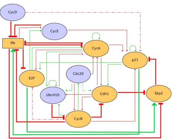
2. TEMPORAL CONSTRAINTS IN THE LOGICAL FRAMEWORK CycD Rb E2F CycE CycA CycB p27 Cdc20 Cdh1 UbcH10 Skp2

Figure 2.4: Updated model of the mammalian cell cycle. Red arrows depict negative interactions (inhibitions), green arrows are positive interactions (activations). Nodes are either Boolean (ellipses) or multilevel (rectangle). Logical rules of yellow nodes have been modified compared to the initial model, and thick arrows correspond to modified regulations. Dashed arrows correspond to interactions that have been removed from the model.

Results

We have investigated the asynchronous dynamics of Fauré’s model using model checking and perturbation analysis, and we systematically assessed the results to refine and extend this model so that it better matches reported data. In this respect, we first carefully reviewed the literature to identify relevant novel information.

The potential roles of different phosphorylation states of the protein Rb (Lundberg & Weinber, 1998) was considered through the use of a ternary node (i.e. taking the value 0, 1 and 2). We further assessed an extension of the model considering the role of Skp2, which links three key inhibitors of the cell cycle and constitutes an additional pathway by which Rb can arrest the progression of the cell cycle [Binné et al., 2007, Liu et al., 2008]. The regulatory graph of the updated model is depicted on Figure 2.4, while the corresponding logical rules are listed in Table 2.2.

Updating of regulatory rules

The cdk inhibitor p27 plays a critical role in several phases of the cell cycle and in the regulation of the quiescent state. It inhibits the activities of cyclin E/cdk2 and cyclin A/cdk2. This inhibitory activity is modeled by opposite regulations on the targets of CycE and CycA. Moreover, p27 and cyclin D also bind in a complex, but this complex retains the activity of cyclin D. Since the cyclins are in competition for complexation with p27, the initial model considered a direct inhibition of

2.4. Application: studying the structural properties of the cell cycle

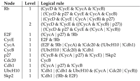
Node Level Logical rule

Rb 1 (CycD & !CycE & !CycA & !CycB) | (!CycD & p27 & CycE & CycA & CycB) | (CycD & (CycE | CycA | CycB) & p27) 2 (!CycD & !CycE & ((!CycA & !CycB) | p27))

| (!CycD & p27 & CycE & (!CycA | !CycB)) E2F 1 (!CycA | p27) & !Rb

CycE 1 E2F & !Rb

CycA 1 (E2F & !Rb | CycA) & !Cdc20 & (!UbcH10 | !Cdh1) CycB 1 (!UbcH10 | !Cdc20) & !Cdh1

p27 1 (!CycB & (!CycA | p27) & !CycE) | !Skp2

Cdc20 1 CycB

Cdh1 1 (!CycA | p27) & !CycB

UbcH10 1 !Cdh1 | (Cdh1 & UbcH10 & (CycA | Cdc20 | CycB)) Skp2 1 !Cdh1 | (!Rb & E2F)

Table 2.2: Logical rules governing transitions in the updated model of the mammalian cell cycle.

p27 by cyclin D to reflect the sequestration of the inhibitor by the cyclin D during the cell cycle. This causes p27 to be completely inactive in presence of the input cyclin D, while it is released and active in absence of the input (i.e. in the quiescent state). This approximation overlooks the role of p27 in the transition from G1 to S. Indeed, the complete activation of cyclin E is a progressive process, slowed down by both Rb and p27, which are both negative regulators of cyclin E: Rb binds to the transcription factor E2F, thereby inhibiting its ability to activate the synthesis of cyclin E, whereas p27 directly binds to cyclin E/Cdk2 and thereby blocks its activity. Rb and p27 are both phosphorylated by cyclin E, inducing inactivity of Rb and proteasome-dependent degradation of p27. These factors are thus involved in a positive circuit enabling the full activation of the kinase and ultimately entry into S phase [Kotoshibai et al., 2005].

In order to account for this mechanism, we removed the inhibition of p27 by CycD. Although it is clear that cyclin D plays a role in p27 phosphorylation, the observation that the activity of p27 varies in the cell cycle while the level of cyclin D stays consistently high suggests that this role is weak relatively to those of cyclin A, cyclin E and cyclin B [Rivard et al., 1996]. Alternatively, a ternary node could have been associated with p27 to distinguish two activation levels, in presence versus absence of cyclin D. We have further modified the rule for p27 (see Table 1) to account for the inhibitory effect of CycE [Montagnoli et al., 1999]. Simulation of the model with this new rule results in a correct asynchronous attractor with varying p27 activity (in the presence of CycD).

In order to verify the correct role of p27 in the cycle, we check for the existence of the three state transition sequences defined in Table 2.3 and formalized with CTL formulae. For example, the sequence of states [001, 101, 100, 110, 010] taken by the vector (CycE, CycA, p27) is translated into the CTL formula:

¬E[ (CycE=0 ∧ CycA=0 ∧ p27=1) U (CycE=1 ∧ CycA=0 ∧ p27=1 ∧E[ (CycE=1 ∧ CycA=0 ∧ p27=1) U (CycE=1 ∧ CycA=0 ∧ p27=0 ∧E[(CycE=1 ∧ CycA=0 ∧ p27=0) U (CycE=1 ∧ CycA=1 ∧ p27=0 ∧E[(CycE=1 ∧ CycA=1 ∧ p27=0) U (CycE=0 ∧ CycA=1 ∧ p27=0)])])])]

This first sequence represents the expected sequence for the G1/S transition, while the other two correspond to incorrect situations where p27 is either degraded before the activation of its inhibitor CycE, or stays active after the activation of CycA. We further impose the constraint CycB=0 & Cdh1=1, characterizing G0, at the initial states.

The requirement of cyclin E for cell cycle viability might depend on the cell context. Cyclin E is known to participate in the phosphorylation of Rb together with cyclin D [Weinberg, 1995]. However, observations on cyclin E-deficient cells highlight a crucial role of cyclin E in some sit-uations. [Geng et al., 2003] reported that cyclin E-deficient cells can maintain active proliferation