• Aucun résultat trouvé

A certified numerical algorithm for the topology of resultant and discriminant curves

N/A
N/A
Protected

Academic year: 2021

Partager "A certified numerical algorithm for the topology of resultant and discriminant curves"

Copied!
27
0
0

Texte intégral

(1)

HAL Id: hal-01402194

https://hal.inria.fr/hal-01402194

Submitted on 24 Nov 2016

HAL is a multi-disciplinary open access

archive for the deposit and dissemination of

sci-entific research documents, whether they are

pub-lished or not. The documents may come from

teaching and research institutions in France or

abroad, or from public or private research centers.

L’archive ouverte pluridisciplinaire HAL, est

destinée au dépôt et à la diffusion de documents

scientifiques de niveau recherche, publiés ou non,

émanant des établissements d’enseignement et de

recherche français ou étrangers, des laboratoires

publics ou privés.

A certified numerical algorithm for the topology of

resultant and discriminant curves

Rémi Imbach, Guillaume Moroz, Marc Pouget

To cite this version:

Rémi Imbach, Guillaume Moroz, Marc Pouget. A certified numerical algorithm for the topology of

resultant and discriminant curves. Journal of Symbolic Computation, Elsevier, 2016, 80, Part 2,

pp.285–306. �10.1016/j.jsc.2016.03.011�. �hal-01402194�

(2)

A certified numerical algorithm for the topology of resultant and

discriminant curves

R´emi Imbacha,b, Guillaume Moroza,b, Marc Pougeta,b

aInria, France. bLORIA laboratory, Nancy, France.

Abstract

Let C be a real plane algebraic curve defined by the resultant of two polynomials (resp. by the discriminant of a polynomial). Geometrically such a curve is the projection of the intersection of the surfaces P(x, y, z)= Q(x, y, z) = 0 (resp. P(x, y, z) = ∂P∂z(x, y, z) = 0), and generically its singularities are nodes (resp. nodes and ordinary cusps). State-of-the-art numerical algorithms compute the topology of smooth curves but usually fail to certify the topology of singular ones. The main challenge is to find practical numerical criteria that guarantee the existence and the uniqueness of a singularity inside a given box B, while ensuring that B does not contain any closed loop of C. We solve this problem by first providing a square deflation system, based on subresultants, that can be used to certify numerically whether B contains a unique singularity p or not. Then we introduce a numeric adaptive separation criterion based on interval arithmetic to ensure that the topology of C in B is homeomorphic to the local topology at p. Our algorithms are implemented and experiments show their efficiency compared to state-of-the-art symbolic or homotopic methods.

1. Introduction

Given a bivariate polynomial f with rational coefficients, a classical problem is the compu-tation of the topology of the real plane curve C= {(x, y) ∈ R2| f (x, y)= 0}. One may ask for the

topology in the whole plane or restricted to some bounding box. In both cases, the topology is output as an embedded piecewise-linear graph that has the same topology as the curve C. For a smooth curve, the graph is hence a collection of topological circles or lines; for a singular curve, the graph must report all the singularities: isolated points and self-intersections.

Symbolic methods based on the cylindrical algebraic decomposition can guarantee the topol-ogy of any curve. However, the high complexity of these purely algebraic methods prevents them to be applied in practice on difficult instances. On the other hand, purely numerical methods such as curve tracking with interval arithmetic or subdivision are efficient in practice for smooth curves but typically fail to certify the topology of singular curves. A long-standing challenge is to extend numerical methods to compute efficiently the topology of singular curves.

Computing the topology of a singular curve can be done in three steps.

Email addresses: Remi.Imbach@inria.fr (R´emi Imbach), Guillaume.Moroz@inria.fr (Guillaume Moroz), Marc.Pouget@inria.fr (Marc Pouget)

(3)

1. Enclose the singularities in isolating boxes.

2. Compute the local topology in each box, that is i) compute the number of real branches connected to the singularity, ii) ensure that it contains no other branches.

3. Compute the graph connecting the boxes.

Up to homeomorphisms, the local topology at a point of a curve is characterized by the number of real (half-) branches of the curve connected to the point. This number is two for a regular point, and can be any even number at a singular point. We define a witness box of a singular point as a box containing the singular point such that the topology of the curve inside the box is the one of the graph connecting the singularity to the crossings of the curve with the box boundary. The topology of the curve in a witness box is thus completely determined by its number of crossings with the box boundary. In this article, we only focus on the first two steps of the above-mentioned topology algorithm, that is computing witness boxes. The third step can be seen as reporting the topology of a smooth curve in the complement of the witness boxes of the singular points. There already exist certified algorithms for this task using subdivision (Plantinga and Vegter(2004);Lin and Yap(2011)). Another option is to use certified path tracking (e.g. Martin et al.(2013);Van Der Hoeven(2011); Beltr´an and Leykin(2013)) starting at the crossings of the curve with the boundary of singularity boxes, note that to report the closed loops without singularity, at least one point on such components must be provided. Contribution and overview.. The specificity of the resultant or the discriminant curves computed from generic surfaces is that their singularities are stable, this is a classical result of singularity theory due to Whitney. The key idea of our work is to show that, in this specific case, the over-determined system defining the curve singularities can be transformed into a regular well-constrained system of a transverse intersection of two curves defined by subresultants. This new formulation can be seen as a specific deflation system that does not contain spurious solutions.

Our contribution focuses on the first two steps of the above mentioned topology algorithm for a curve defined by the resultant of two trivariate polynomials P and Q: f= Resultantz(P, Q),

see Figure1for an illustration of the discriminant curve of a torus.

In Section2, the main results are Theorems1and2that characterize the singularities of the resultant or discriminant curve in terms of subresultants under generic assumptions. A semi-algorithm1 is proposed to check these generic assumptions, i.e. it terminates if and only if the assumptions are satisfied (note that this is the best one can hope for when using a purely numerical method). Based on the characterization of Theorems1 and2, Algorithm 2, using subdivision and interval evaluation, isolates the node and cusp singularities with an adaptive certification.

Sections3and4address the second step on the above-mentioned topology algorithm. Algo-rithms3and4in Section3distinguish nodes from cusps and compute the number of branches. Then in Section4, Algorithm5refines an isolating box of a singular point such that it becomes a witness box.

In Section5, experiments are detailed showing that our specialized certified numerical method outperforms state-of-the-art implemented methods for polynomials of degree greater or equal to 5. Moreover, the performance of our method is also improved when we restrict the problem to a box.

Notations.. Let f be a bivariate polynomial and C it associated curve. We denote by fxiyj the

partial derivative (∂x)∂i+ ji(∂y)f j. A point p= (α, β) in C

2is singular for f if f (p)= f

x(p)= fy(p)= 0,

(4)

and regular otherwise. A node is a singular point with det(Hessian( f ))= f2

xy− fx2fy2 6= 0. An

ordinary cuspis a singular point such that det(Hessian( f ))= 0 and for all non trivial direction (u, v), f (α+ ut, β + vt) vanishes at t = 0 with multiplicity at most 3.

We denote by f any convergent interval extension of f , that is for any box B, { f (x, y)|(x, y) ∈ B} ⊂ f (B), and for any decreasing sequence of boxes Biconverging to a point p, the sequence

 f (Bi) converges to f (p). By abuse of notation, we often denote f (B) by Bf or simply f .

The Krawczyk operator of a mapping F defined in Lemma7is denoted by KF. The topological

interior of a box B is denoted int(B).

For two polynomials P and Q in D[z] with D a unique factorization domain (in this article D will be Q[x, y]), recall that the ithsubresultant polynomial is of degree at most i (see e.g. (Kahoui,

2003, §3)), we denote it Si(z)= siizi+ si,i−1zi−1+ · · · + si0. The resultant is thus S0(z)= s00in D

and we also denote it more classically as Resz(P, Q). Finally, V( f1, . . . , fn) denotes the solutions

of the system f1= · · · = fn= 0.

Previous and related work.. There are many works addressing the topology computation via symbolic methods, see for instance the book chapter byMourrain et al.(2006) and references therein. Most of them use subresultant theory, but there are also some alternatives using only resultants (e.g. Seidel and Wolpert (2005); Emeliyanenko and Sagraloff (2012)) or Gr¨obner bases and rational univariate representations (Cheng et al.(2010)). An alternative byAkoglu et al.(2014) even computes a rational univariate representation numerically if all approximate solutions are known. For the restricted case of computing the topology of non-singular curves, certified numerical methods are usually faster and can in addition reduce the computation to a user defined bounding box. One can mention interval analysis methods (Martin et al.(2013)) or more generally certified homotopy methods (Beltr´an and Leykin(2013); Van Der Hoeven

(2011)). These methods are based on the fact that the regular solutions of a square system can be certified and approximated with quadratic convergence with the interval Newton-Krawczyk oper-ator (Rump(1983);Neumaier(1990)). Another well-studied numerical approach is via recursive subdivision of the plane. Indeed, the initial idea of the marching cube algorithm byLorensen and Cline(1987) can be further improved with interval arithmetic to certify the topology of smooth curves (Snyder(1992);Plantinga and Vegter(2004);Liang et al.(2008)).

For singular curves, isolating the singular points is already a challenge from a numerical point of view. Indeed, singular points are defined by an over-determined system f = fx= fy= 0

and are not necessarily regular solutions of this system. A classical approach to handle an over-determined system { f1, . . . , fm} is to combine its equations in the form f1 xif1 + · · · + fm xifm =

0 for each variable {xi}1≤i≤n<m, to transform it into a square system (Dedieu(2006)), but this

introduces spurious solutions. Singular solutions can be handled through deflation (Giusti et al.

(2007); Ojika et al.(1983);Leykin et al.(2006);Mantzaflaris and Mourrain (2011)), roughly speaking, the idea is to compute partially the local structure of a non-regular solution, and use this information to create a new system where this solution is regular. However this system is usually still overdetermined, and it does not vanish on the solutions of the original system that do not have the same local structure. Thus, this cannot be directly used to separate solutions with different multiplicity structures. It is important to mention that the certification of solutions of over-determined systems is theoretically out of reach of numerical methods in the general case. In the polynomial case, non-adaptive lower bounds can be used but they are too pessimistic to be practical, see (Hauenstein and Sottile,2012, Remark 7) orBurr et al.(2012).

When the curve we consider is a resultant, its singular locus can be related to the first sub-resultant (see (Jouanolou, 1979, §4.3) and (Bus´e and Mourrain,2009, §5) for examples). In

(5)

Section2, we use this structure to exhibit a square deflation system. Another approach would be to exhibit a square system in higher dimension that defines the set of points for which the poly-nomials P and Q have two solutions. This approach was considered byDelanoue and Lagrange

(2014) to compute the topology of the apparent contour of a smooth mapping from R2to R2.

The number of real branches connected to the singularity can be computed with the topo-logical degree of a suitable mapping (Szafraniec(1988);Alberti et al.(2008);Mantzaflaris and Mourrain(2011)) or with the fiber multiplicity together with isolation on the box boundary ( Sei-del and Wolpert(2005)). Certifying the topology inside a box requires the detection of loops near a singularity. It is usually solved in the literature by isolating the x-extreme points, which reduces the problem to a univariate polynomial computed with resultants (Seidel and Wolpert

(2005);Mourrain et al.(2006) for example).

We are not aware of numerical algorithms that can certify in practice the computation of the topology of singular curves, but several promising approaches have been presented. Relying on global non-adaptive separation bounds for algebraic systems, the subdivision approach presented byBurr et al.(2012) can theoretically certify the topology of any singular curve. Due to these worst-case bounds, this algorithm cannot be practical. A numerical algebraic geometric approach is presented byLu et al.(2007) using irreducible decomposition, generic projection and plane sweep, deflation and homotopy to compute the topology of a singular curve in any codimension. Even if this work has been implemented byBates et al.(2013)1, the certification of all the

al-gorithm steps appears as a challenge. The numerical approach byCorless et al.(2013), based on Bezoutian and eigenvalue computation, can handle singular curves but even if multiprecision gives accurate results no certification is provided.

2. Subresultant based deflation

The input of algorithms in this section are two trivariate polynomials P, Q and a box B0 in

R2. Our goal is to isolate the singularities of the plane curve f = 0 defined by the resultant of Pand Q with respect to z. In this section, we exhibit a square polynomial system g = h = 0 and a polynomial u such that the singularities of f are exactly the solutions of the constrained system g= h = 0 and u 6= 0. Moreover, the singularities are regular solutions of g = h = 0, such that numerical methods can certify whether a box contains or not a singularity. In Section2.1, the constrained system is constructed using subresultants. In Section2.2, the regularity of this system is translated in terms of types of singularities. Generic assumptions are required so that these characterizations of the singularities of f hold. Section2.3presents a semi-algorithm for checking the assumptions that we now define. Given two trivariate polynomials P, Q in Q[x, y, z] and a two-dimensional box B0, we define the generic assumptions:

(A1) Above the box B0for the x and y-coordinates, the intersection of the surfaces P(x, y, z)= 0

and Q(x, y, z) = 0 is a smooth space curve denoted CP∩Q, i.e. the tangent vector t =

OP × OQ is nowhere null on CP∩Q(whereOP is the gradient vector (Px, Py, Pz)).

(A2) Above any point (α, β) in B0, there are at most two points of CP∩Qcounted with

multiplic-ities, or in other words, the polynomial gcd(P(α, β, z), Q(α, β, z)) has degree at most two. In addition, there are finitely many (α, β) in B0such that this degree is two.

1See alsowww.bertinireal.comandMyszka et al.(2013) for an application to real curves arising in engineering.

(6)

(A3) The leading coefficients LP(x, y) and LQ(x, y) of P and Q seen as polynomials in z have no

common solutions in B0.

(A4) The singularities of the resultant or discriminant curve are only nodes or ordinary cusps.

Note that these assumptions are satisfied for almost all pairs of polynomials in Q[x, y, z]. 2.1. Singularities via subresultants

Let f be the resultant polynomial (with respect to the variable z) of two polynomials P and Qin Q[x, y, z]. We always assume that f is square-free and thus its singularities are isolated. Let Ssing= V( f, fx, fy) be the set of singular points of f and Ssres= V(s11, s10) − V(s22). We prove in

this section that, under our assumptions, these two sets coincide. Figure2illustrates Theorem1

for the discriminant curve of a torus.

Theorem 1 (Recknagel(2013)). Let f be the resultant of the polynomials P and Q in Q[x, y, z] with respect to the variable z. Then Ssres⊂ Ssingand if the assumptions(A1) to (A3) are satisfied

then Ssing ⊂ Ssres.

Proof of the inclusion Ssres ⊂ Ssing.. Let I = h f, fx, fyi and J = hs11, s10i : hs22i∞, then

Ssing = V(I) and V(J) = V(s11, s10) − V(s22) = Ssres ⊃ Ssres. It is thus sufficient to prove

that I ⊂ J, or in other words that there exists a positive integer m such that h f , fx, fyi · hs22im=

hsm 22f, s m 22fx, s m 22fyi ⊂ hs11, s10i.

The generic chain rule of subresultant (see for instance (Kahoui,2003, Theorem 4.1)) yields s2

22f = Res(S2, S1). On the other hand, Res(S2, S1) =

s22 s11 s21 s10 s11 s20 s10 = s2 10s22 + s 2 11s20 − s10s11s21. Hence s222f ∈ hs11, s10i.

The previous identity expresses s222f as a quadratic form in s11and s10, differentiating with

respect to x (or y) yields a sum with s11or s10as a factor in each term, thus ∂(s222f) is in hs11, s10i.

This implies that ∂(s322f) is also in hs11, s10i. In addition, ∂(s322f) = 3s222f∂s22+ s322∂ f hence

s322∂ f = ∂(s322f) − 3s222f∂s22with both terms in hs11, s10i, thus s322∂ f is in hs11, s10i. We conclude

that hs322f, s322fx, s223 fyi ⊂ hs11, s10i, hence I ⊂ J and Ssres⊂ Ssing.

Proof of the inclusion Ssing ⊂ Ssres.. Let (α, β) be a singular point of f , so that f (α, β) = 0.

According to the generic condition (A2), gcd(P(α, β, z), Q(α, β, z)) has at most two simple roots

or one double root.

For the case of a double root, gcd(P(α, β, z), Q(α, β, z)) has degree 2 and by the gap structure theorem (more precisely its corollary showing the link between the gcd and the last non-vanishing subresultant, see e.g. (Kahoui,2003, Corollary 5.1)) and assumption (A3): (a) this gcd is the

sub-resultant S2(α, β), hence s22(α, β) 6= 0, and (b) the subresultants of lower indices are vanishing,

in particular s11(α, β)= 0 and s10(α, β)= 0. Hence (α, β) is in Ssres.

Otherwise, let γ be a simple root of gcd(P(α, β, z), Q(α, β, z)), the generic condition (A1)

yields that the tangent vector t(p) to CP∩Q at the point p = (α, β, γ) is well defined and not

vertical. Indeed, the multiplicity of γ in gcd(P(α, β, z), Q(α, β, z)) is 1, so it is also 1 in at least one of the polynomials P(α, β, z) or Q(α, β, z). In other words, Pz(p) 6= 0 or Qz(p) 6= 0 which

implies that the x and y-coordinates of t(p) cannot both vanish (otherwise, t(p) would be the null vector contradicting assumption (A1)). Without loss of generality we may assume that the

x-coordinate of t(p) is not null: xt(p) = Py(p)Qz(p) − Pz(p)Qy(p) 6= 0.

(7)

Figure 1: A torus defined by P= 0, in dashed line the curve P = Pz= 0 and in solid line the discriminant curve of the

torus defined by Resz(P, Pz)= 0.

Figure 2: Illustration of Theorem1. Two views of the discriminant curve f = 0 of the torus of Figure1and curves defined by the coefficients s10, s11, s22of the sub-resultants chain of P and Pz. The singularities of the discriminant

curve are the solutions of the system s11= s10= 0 such that s22does not vanish.

(8)

We now apply (Bus´e and Mourrain,2009, Theorem 5.1) rephrased in the affine setting to P and Q: fy= ± Py Pz Qy Qz s11+ uP + vQ

with u, v in Q[x, y]. Evaluated at p, P and Q vanish and we obtain: fy(α, β) = ±xt(p)s11(α, β).

Since (α, β) is a singular point of f , fy(α, β)= 0, and together with xt(p) 6= 0 this gives s11(α, β)=

0. The gap structure theorem and f (α, β) = 0 then implies that (a) s10(α, β) = 0, and (b) the

degree of gcd(P(α, β, z), Q(α, β, z)) is at least 2. Together with the generic condition (A2), this

degree is exactly 2 and so is the degree of the second subresultant S2 evaluated at (α, β), thus

s22(α, β) 6= 0. We then conclude that in this case too (α, β) is in Ssres.

2.2. Regularity conditions

The main theorem of this section is the relation between the types of singularities of f and the regularity of the solutions of the system s11 = s10 = 0. We assume for this section that the

assumptions (A1), (A2) and (A3) hold.

Theorem 2. Let f be the resultant of the polynomials P and Q in Q[x, y, z] with respect to the variable z. If the assumptions(A1), (A2) and (A3) hold then the following propositions are

equivalent:

i. p is a regular solution of s11 = s10= 0 and s22(p) 6= 0

ii. p is a node or an ordinary cusp of the curve f = 0

Furthermore in this case, p is an ordinary cusp point if and only if CP∩Qhas a vertical tangent

above p.

The proof of this theorem is decomposed with the following lemmas.

Lemma 3 (Recknagel(2013)). Let p be a node of f . Then p is a regular point of the system s11= s10= 0.

Proof. Since p is a node, it is a singular point of f = 0 and Theorem1implies that p is a solution of the system s11 = s10 = 0. Moreover, we saw in the proof of Theorem1that Ssres ⊂ Ssing

but more precisely that hs322f, s322fx, s322fyi ⊂ hs11, s10i. In the following, we use the notion of

multiplicity of a point in an ideal sometimes called the intersection multiplicity as defined for instance in (Cox et al.,2005, §4.2, Definition 2.1). In particular, the latter inclusion implies that the multiplicity of p in hs11, s10i is lower or equal to its multiplicity in hs322f, s322fx, s322fyi. Since

pis a node of f , the determinant of the Hessian of f is non-zero and p is a regular point of h f, fx, fyi. And since s22(p) 6= 0, we can conclude that the multiplicity of p in hs322f, s322fx, s322fyi

is 1. Thus p has also a multiplicity 1 in hs11, s10i.

Lemma 4. Let p be an ordinary cusp point of f . Then p is a regular point of the system s11 =

s10= 0.

Proof. Let p = (α, β) be an ordinary cusp point of f . Suppose by contradiction that p is a singular solution of s11 = s10 = 0. Then the determinant of the Jacobian matrix

s11 xs10 x

s11 ys10 y

 is 0 and there exists a vector (u, v) ∈ R2\ {(0, 0)} orthogonal simultaneously to the gradient of s11and

to the gradient of s10. In particular, s11(α+ ut, β + vt) (resp. s10(α+ ut, β + vt)) vanishes at 0 in

(9)

twith multiplicity at least 2. Using standard formula on the resultants ((Kahoui,2003, Theorem 4.1) for example) we have s2

22f = Res(S1, S2). Developing the right hand side we get:

s222f = s22s210− s21s11s10+ s20s211.

Thus, evaluating the right hand side on (α+ ut, β + vt), we observe that it vanishes at 0 in t with multiplicity at least 4.

On the other hand, p being an ordinary cusp of f , the polynomial f (α+ ut, β + vt) vanishes at 0 in t with multiplicity at most 3. In addition, under the assumptions (A2) and (A3), we

have s22(p) 6= 0 and the left hand side vanishes at 0 in t with multiplicity at most 3, hence a

contradiction follows.

Lemma 5. Let q = (α, β, γ) be a regular point of the curve CP∩Q such that s22(p) 6= 0 with

p = (α, β). Then q is a regular point of the curve S2(x, y, z) = S1(x, y, z) = 0. Moreover, the

vectors ∇P(q), ∇Q(q) generate the same vector space as ∇S2(q) and ∇S1(q).

Proof. Using the identities of (Kahoui,2003, Theorem 4.2), there exists U, V, U0, V0such that: s222P= US2+ VS1 s222Q= U0S2+ V0S1 Since s22(p) 6= 0, we have: ∇P(q)= U(q) s22(p)2 ∇S2(q)+ V(q) s22(p)2 ∇S1(q) ∇Q(q)= U0(q) s22(p)2 ∇S2(q)+ V0(q) s22(p)2 ∇S1(q)

Since q is a regular point of P= Q = 0, ∇P(q) and ∇Q(q) generate a dimension 2 vector space. Thus ∇S2(q) and ∇S1(q) also generate the same dimension 2 vector space and q is a regular point

of the curve S2= S1= 0.

Proof of Theorem2. The implication ii. =⇒ i. is a direct corollary of Lemma3and4. For the reciprocal, we know that s22(p) 6= 0, thus

f = 1 s22 s210+ 1 s2 22 s20s211− 1 s2 22 s21s10s11

Let us denote by A, J and V the matrices and the vector A= 2s22 −s21 −s21 2s20 ! J= s10 x s10y s11 x s11cy ! V = s10 s11 !

The resultant satisfies f= 1 2s2

22

Vt· A · V. Let p be a singular point of the curve f = 0. According to Theorem1, s11(p)= s10(p)= 0. Moreover, without restriction of generality, we can assume

that (α, β, 0) satisfy P(α, β, 0)= Q(α, β, 0) = 0 using the property that the resultant is invariant by translation of z in P and Q. In this case, we have also s20(p)= 0.

With abuse of notations, we denote by Ok(x, y) a polynomial that is in the ideal hx, yikwhere

kis a positive integer. In particular we have:

Ok1(x, y) · Ok2(x, y)= Ok1+k2(x, y)

Ok1(x, y)+ Ok2(x, y)= Omin(k1,k2)(x, y)

δOk(x, y)= Ok−1(x, y) for δ= ∂/∂xor ∂/∂y

(10)

With this notation, the taylor expansion of V at p gives V(p+ (x, y)) = J(p) x y ! + O2(x, y) such that : f(p+ (x, y)) = 1 2s22(p)2 (x y) J(p)t· A(p) · J(p) x y ! + O3(x, y)

This implies that the Hessian of f at p is the matrix s 1

22(p)J(p)

t· A(p) · J(p). If the determinant

of the Hessian is not zero, then p is a node. Otherwise we have det(A(p)) det(J(p))2 = 0. Let

us prove in this case that p is an ordinary cusp in f . For that, we need to prove that for every direction (u, v) 6= (0, 0), the valuation of t in f (p + t(u, v)) is lower or equal to 3. By hypothesis i., det(J) 6= 0, thus det(A(p)) = 4s22(p)s20(p)− s21(p)2= 0. In particular, this means that s21(p)= 0.

In particular recalling that:

f = 1 s22 s210+ 1 s222s20s 2 11− 1 s222s21s10s11 we have for (u, v) such that a := us10 x(p)+ vs10y(p) 6= 0:

s210(α+ ut, β + vt) = a2t2+ O3(t) s20s211(α+ ut, β + vt) = O3(t) s21s10s11(α+ ut, β + vt) = O3(t) This implies: f(α+ ut, β + vt) = 1 s22(p) a2t2+ O3(t)

and for (u, v) such that us10 x(p)+ vs10y(p)= 0 there exists a constant c 6= 0 such that (u, v) = (cs10y, −cs10 x) and we have:

f(α+ ut, β + vt) = c

3

s22(p)2

(s20 x(p)s10y(p) − s20y(p)s10 x(p))(s11 x(p)s10y(p) − s11y(p)s10 x(p))2t3

+ O4(t) = c3 s22(p)2 det(G(p)) det(J(p))2t3+ O4(t) where G:= s20 x s20y s10 x s10y !

Lemma5 implies that (α, β, 0) is a regular point of S2(x, y, z) = S1(x, y, z) = 0. On the other

hand, ∇S1(α, β, 0)=  s10 x(p) s10y(p) s11(p)  ∇S2(α, β, 0)=  s20 x(p) s20y(p) s21(p)  9

(11)

Since s11(p) = s21(p) = 0, the point (α, β, 0) is regular in S2(x, y, z) = S1(x, y, z) = 0 only

if the determinant of the matrix G(p) is different from zero. In addition, hypothesis i. implies det(J(p)) 6= 0. We thus conclude that for every (u, v) 6= (0, 0), the valuation of t in f (ut, vt) is lower or equal to 3, and p is an ordinary cusp.

Finally, we prove that p is an ordinary cusp if and only if CP∩Qhas a vertical tangent above p

at q= (α, β, 0). First, if p is an ordinary cusp, then the Hessian of f is zero at p and det(A(p)) = 0. In this case we saw that s21(p)= 0 and since s11(p)= 0, this implies that ∂S∂z2(q)= s21(p)= 0

and ∂S1

∂z (q) = s11(p) = 0. Using Lemma5this implies that ∂P∂z(q) = ∂Q∂z(q) = 0 such that the

tangent vector of CP∩Qat q is vertical. Reciprocally, if the tangent vector of CP∩Qat q is vertical,

then∂P∂z(q)= ∂Q∂z(q)= 0 and Lemma5implies that∂S2

∂z (q)= 0, thus S2has a double root in z and

det(A(p))= 0. Thus the Hessian of f is vanishing at p and p is an ordinary cusp of f . 2.3. Checking the assumptions

As opposed to symbolic methods, our numerical approach requires assumptions on the input. To be complete we provide a way to check that the assumptions are fulfilled using only numerical methods. Note that we only provide a semi-algorithm, when it halts one is sure that the assump-tions are satisfied. On the other hand, if it is stopped at an arbitrary time threshold, no result is provided. In addition, when the assumptions are satisfied the running time could be considered as a measure of how near the input is from the degenerate ones, that is the set of inputs that do not satisfy the assumptions.

Lemma 6. The semi-algorithm1terminates if and only if the assumptions(A1), (A2), (A3) and

(A4) are satisfied.

Proof. We first show that if the semi-algorithm terminates then (A1), (A2), (A3) and (A4) are

satisfied. Indeed, for any box of the subdivision, (a) Lines5ensures that the leading coefficients LPand LQof P and Q have no common solutions so that (A3) holds; (b) Lines7,9and15ensure

that f , s11 and s22 do not vanish simultaneously, hence there is at most two points of the curve

CP∩Qabove each point of B0, (A2) is satisfied; (c) Lines11and17ensure that the curve CP∩Qis

smooth so that (A1) holds; Line19finally ensures the regularity assumption (A4).

Conversely, it is easy to see that when the assumptions (A1), (A2), (A3) and (A4) are satisfied

Semi-algorithm1 will terminate due to the convergence of the interval functions to the actual value of the corresponding function when the diameter of a box tends to 0.

2.4. Numerical certified isolation

There is no new result in this section, but for the reader’s convenience, we recall a classical numerical method to isolate regular solutions of a square system within a given domain via recur-sive subdivision and show how it applies in our case. Such a subdivision method is often called branch and bound method (Kearfott (1996)) and uses the Krawczyk operator or Kantorovich theorem to certify existence and unicity of solutions. We recall the properties of the Krawczyk operator and propose the naive Algorithm2for the isolation of the singularities of a resultant using the characterization of these points proved in Theorem2. Note that even if the assump-tions (A1) to (A4) are satisfied, this naive algorithm may fail if a singularity lies on (or near) the

boundary of a box during the subdivision. Indeed, for this algorithm to be certified, there is a need to use ε-inflation of a box when using the Krawczyk test and cluster neighboring boxes of

(12)

Semi-algorithm 1 Subdivision based checking of assumptions (A1), (A2), (A3) and (A4)

Input: A box B0in R2and two polynomials P and Q in Q[x, y, z].

Output: The semi-algorithm terminates if and only if the assumptions (A1), (A2), (A3) and (A4)

are satisfied.

1: Let f be the resultant and s22, s11, s10be the subresultant coefficients of P and Q wrt z.

2: L:= {B0}

3: repeat

4: B:= L.pop

5: if 0 ∈LP(B) and 0 ∈LQ(B) then . Checking (A3)

6: Subdivide B and insert its children in L, continue

7: else if 0 6∈ f (B) then .Checking if P and Q have no common solution(A2)

8: continue

9: else if 0 6∈s11(B) then .Checking if P and Q have at most 1 common solution(A2)

10: Iz:= −s10(B)/s11(B)

11: if (0, 0, 0) ∈t(B × Iz) then . Checking (A1)

12: Subdivide B and insert its children in L, continue

13: else

14: continue

15: else if 0 6∈s22(B) then .Checking if P and Q have at most 2 common solutions(A2)

16: Iz:= union of the complex boxes solution of: s22(B)z2+ s21(B)z+ s20(B)= 0

17: if (0, 0, 0) ∈t(B × Iz) then . Checking (A1)

18: Subdivide B and insert its children in L, continue

19: else if 0 ∈Jacobian(s11, s10)(B) then . Checking (A4)

20: Subdivide B and insert its children in L, continue

21: else

22: continue

23: else

24: Subdivide B and insert its children in L, continue

25: until L= ∅

26: return true

the subdivision. For simplicity we do not detail this issue and refer for instance to (Stahl,1995, §5.9),Kearfott(1997);Schichl and Neumaier(2005).

Let F be a mapping from R2to R2and denote JFits Jacobian matrix. The following lemma

is a classical tool to certify existence and uniqueness of regular solutions of the system F=0 0

 . For simplicity, we state the following lemma on R2but this result holds in any dimension.

Lemma 7. (Krawczyk Krawczyk(1969)(Rump,1983, §7)) Let Bx, By be real intervals, B =

(Bx, By) be a box in R2, (x0, y0) be the center point of B and ∆B =

Bx−x0 By−y0  . Let N be the mapping: N(x, y)= xy − JF(x0, y0)−1· F(x, y)

and KF the Krawczyk operator defined by:

KF(B) := N(x0, y0)+ JN(B) ·∆B.

If KF(B) is contained in the interior of B then F=

0

0


has a unique solution in B. 11

(13)

Algorithm 2 Subdivision based isolation of singularities

Input: A box B0 in R2 and two polynomials P and Q in Q[x, y, z] such that the assumptions

(A1), (A2), (A3) and (A4) are satisfied.

Output: A list LS ing of boxes such that each box isolates a singularity of the curve defined by

f = Resz(P, Q), and each singularity in B0is in a box of LS ing.

1: Let f be the resultant and s22, s11, s10be the subresultant coefficients of P and Q wrt z.

2: L:= {B0} 3: repeat 4: B:= L.pop 5: if 0 6∈ f (B) or 0 6∈ s11(B) or 0 6∈s10(B) then 6: Discard B 7: else

8: if K(s11,s10)(B) ⊂ int(B) and 0 6∈s22(B) then 9: Insert B in LS ing

10: else

11: Subdivide B and insert its children in L

12: until L= ∅

13: return LS ing

The Krawczyk operator can be seen as the mean value evaluation of the Newton mapping. This implies that the refinement, by recursively applying the Krawczyk operator, of a box con-taining a unique solution is quadratically convergent (Moore and Jones(1977)). We use such a refinement in Algorithms3,4and5.

Termination of Algorithm2.. We assume that P, Q satisfy the assumptions (A1), (A2), (A3) and

(A4). Since in this case the singularities of f are either nodes or ordinary cusp points, Theorem2

implies that they are regular solutions of the system s11 = s10= 0. This implies that Algorithm2

will always terminate.

3. Number of real branches at singularities

Algorithm2isolates singularities in boxes. The next step is to identify the singularity type, node or ordinary cusp, and compute its local topology i.e. the number of real branches of the curve connected to the singular point.

3.1. Resultant

For a resultant curve, recall that nodes are stable singularities whereas cusps are not, thus a purely numerical method cannot distinguish between node and cusp singularities. In particular, given a box B containing a singularity, let I be a box evaluation of the determinant of the Hessian. If I does not vanish in the considered box, it is a node, but if it contains 0, it can still be a node, but also a cusp. For a node, the local topology is easily deduced from the topological degree of the mapping ( fx, fy).

Lemma 8. (Alberti et al.,2008, Theorem 4.15) Let B be a box containing a singularity p of f such that I:=  det(H)(B) 6= 0, then if I < 0 then p is connected to 4 real branches, otherwise if I> 0, then p is an isolated real point.

(14)

Conversely, if p is a node, then for a small enough box containing p, the determinant of the Hessian does not contain 0 and the number of branches connected to p can be recovered. Thus, when B contains a node singularity of the resultant, Semi-algorithm3will always terminate and compute the number of real branches connected to p. Note that in the case when the singularity is an ordinary cusp, Semi-algorithm3will not terminate.

Semi-algorithm 3 Number of branches at a resultant singularity

Input: A box B in R2output by Algorithm2containing a unique singular point p.

Output: The number of branches connected to p.

1: Let f be the resultant and s11, s10be the subresultant coefficients of P and Q wrt z.

2: while 0 ∈ det(Hessian( f ))(B) do

3: B:= B ∩ K(s11,s10)(B)

4: if  det(Hessian( f ))(B) > 0 then return 0

5: else return 4

3.2. Discriminant

In this section we focus on a discriminant curve. Let f be the resultant of P and Q := Pz

satisfying the assumptions (A1), (A2), (A3) and (A4).

The discriminant of P is equal to the resultant of P and Pzdivided by the leading term of P in

z. Assumption (A3) implies that the leading coefficient of P in z is constant, such that the curve

defined by f is the same as the one defined by the discriminant of P.

As for the resultant, the singularities of the curve f = 0 are either nodes or ordinary cusps. Furthermore, for the discriminant curve, the ordinary cusps are stable and we can identify them numerically. Node singularities can be detected and their local topology computed with the same algorithm as in the previous section for the resultant. We will now focus on the case where the singular point is an ordinary cusp. First we show that above an ordinary cusp, the polynomial P has a triple root in z.

Lemma 9. Under the assumptions (A1), (A2), (A3), (A4) the point p= (α, β) is an ordinary cusp

of the discriminant curve f = 0 if and only if P(α, β, z) has a triple root in z.

Proof. Under our assumptions, Theorem 2 states that p = (α, β) is an ordinary cusp of the discriminant curve f = 0 if and only if the curve CP∩Pzhas a vertical tangent above p. This is the

case if and only if there exists γ such that Pz(α, β, γ)= Pzz(α, β, γ)= 0. Moreover, (A2) implies

that Pzzz(α, β, γ) 6= 0, such that γ is a triple root of P(α, β, z).

It is thus desirable to identify cusps via triple points, the following lemma states the regularity of these points which is a necessary condition to use numerical methods for their isolation. Lemma 10. If P has a triple point, and the curve P = Pz = 0 is smooth then the point is a

regular solution of P= Pz= Pzz= 0.

Proof. At the triple point q, the Jacobian of the system P= Pz = Pzz= 0 is Pzzz(q)

Px(q) Pxz(q) Py(q) Pyz(q) . By assumption, Pzzz(q) 6= 0. Moreover, since the curve P = Pz = 0 is regular, at least one minor

of its jacobian matrix is not zero. Since Pz(q)= 0 and Pzz(q)= 0, this means that

Px(q) Pxz(q) Py(q) Pyz(q) 6= 0. Thus the Jacobian is not zero and q is regular.

(15)

The following more effective version of this Lemma delimits the box containing the triple root.

Lemma 11 (triple points). Let B be a box containing a unique singular point p of f and assume that 0 /∈ s22. The polynomial P has a triple point in z above p if and only if the system

P= Pz= Pzz = 0 has a regular solution in the box B × Izwhere Izis the interval −2ss21

22.

Proof. If P(α, β, z) has a triple root z0for (α, β) ∈ B, then it has a multiplicity 2 in gcd(P(α, β, z),

Pz(α, β, z)). In particular z0is a double root of the second polynomial subresultant S2 = s22z2+

s21z+ s20, and z0 = −2ss21(α,β)

22(α,β) ⊂ Iz. Thus if (α, β) is the projection of a triple point of P, then

this point is necessarily in the box B × Iz. Finally if the system P = Pz= Pzz = 0 has a regular

solution in B × Iz, then we can conclude that the 3d box contains a triple point of P and that its

projection is p.

An ordinary cusp is connected to exactly 2 real branches. Using Lemma11, Algorithm4

classifies the singularities between nodes and ordinary cusps, and compute the number of real branches connected to them. It always terminates since the diameter of the box converges toward 0 such that eventually either det(Hessian( f ))(B) 6= 0 or K(P,Pz,Pzz)(B × Iz) ⊂ int(B × Iz).

Algorithm 4 Number of branches at a discriminant singularity

Input: A box B in R2output by Algorithm2containing a unique singular point p.

Output: The number of branches connected to p and its singularity type (node or ordinary cusp).

1: Let f be the resultant and s2,2, s2,1, s11, s10be the subresultant coefficients of P and Pzwrt z.

2: while true do

3: if  det(Hessian( f ))(B) > 0 then return (0, node)

4: if  det(Hessian( f ))(B) < 0 then return (4, node)

5: Iz:= −2ss21(B)

22(B)

6: if K(P,Pz,Pzz)(B × Iz) ⊂ int(B × Iz) then return (2, ordinary cusp) 7: B:= B ∩ K(s11,s10)(B)

4. Loop detection near singularities

Now that we know the number of branches npconnected to a singularity p, we need to ensure

that the enclosing box B computed so far does not contain any other branches not connected to p. First we can refine B until the number of branches crossing the boundary of B matches np.

But this is not enough, since B could contain closed loops of f , see Figure3. This case can be discarded for a node by ensuring that B contains a unique solution of the system fx = fy = 0

(Lemma12), for a cusp we define a specific interval test (Lemma14). 4.1. Resultant

In the case of nodes, p is a regular solution of the system fx= fy= 0 since the determinant

of the Jacobian of this system is the determinant of the Hessian of f and is not zero at p. Thus we can use standard tools from interval analysis to guarantee that p is the only root in B of the system fx= fy= 0.

(16)

B1

B2

B3

s

Figure 3: Illustration for Algorithm5. As input, B1is an isolating box of a node that contains a closed loop of the

resultant curve f= 0. The first refinement of Algorithm5yields a box B2that avoids the point s solution of the system

fx= fy= 0. B2no longer contains the closed loop but is still intersected by branches not connected to the node. The

second refinement of Algorithm5yields the witness box B3.

Lemma 12 (Node near loops). Let K( fx, fy) be the Krawczyk operator defined in Lemma7 with

respect to the system fx= fy= 0, and B be a box containing a node p of f . If K( fx, fy)(B) ⊂ int(B)

then B contains no closed loop of f .

Proof. Lemma 7 ensures that p is the only solution of fx = fy = 0 in B. If B contains a

closed loop included in int(B), then a connected subset of B has its boundary included in the curve defined by f . Thus it contains a point q where f reaches a local extremum and such that

f(q) 6= 0. In particular, fx(q)= fy(q)= 0 and q 6= p, hence the contradiction.

Remark 13. Alternatively, using tools from the next section, denoting by f an evaluation of f on the box B, we let I:=  fxx fyy− fxy fxy. Then we claim that if I does not contain0 then

B contains at most 1 solution of the system fx= fy= 0.

4.2. Discriminant

For the discriminant, the loops near the nodes can be handled as for the resultant. However, the same approach cannot handle ordinary cusps. The problem is that ordinary cusps are singular solutions of the system fx= fy= 0. We need the following lemma to handle ordinary cusps.

Lemma 14 (Ordinary cusp near loops). Let p be an ordinary cusp point of f in a box B. Let J, K, L, M be the intervals:

J=  fyy

K=  fyy2 fxxx− 3 fyy fxy fxxy+ 3 fxy2 fxyy− fxy fxx fyyy

L=  fyy fxxy+  fxx fyyy− 2 fxy fxyy

M=  fyy fxy− fxy fyy

and let J0, K0, L0, M0be the intervals obtained by the same formula with x and y swapped. Let I= JK − LM and I0= J0K0− L0M0. If (J and I) or (J0and I0) do not contain0, then B does not

contain any closed loop of the curve defined by f .

Remark 15. If B is small enough, then either I or I0does not contain zero.

(17)

When a solution of a system S is singular, there are several ways to check that a box B does not contain any other solutions of S . One way is to compute a univariate polynomial r vanishing on the projection of the solutions of S (with resultant or Gr¨obner bases), and check that the projection of B contains only one solution of the square-free part of r. Another way is to use a multivariate version of the Rouch´e theorem (see for instanceVerschelde and Haegemans(1994)). In our case, this would amount to solve a system of two polynomials of degree lower than 3 and check if its solutions are within a suitable complex box containing B.

The method we propose is easy to implement and can potentially be extended to other kinds of functions than polynomials. The main idea behind the proof of Lemma14is to compute a pseudo-resultant of fxand fyin the ring localized at p. Then using the fact that the evaluation on

a box of the coefficients of the Taylor expansion of a polynomial f is included in the evaluation of the corresponding derivative of f , we can compute the evaluation of the local elimination polynomial on B using only derivatives of the polynomials fxand fy.

Before proving Lemma14, we define the notion of separation polynomial that we will use. Definition 16. Let S be a bivariate polynomial system vanishing on p= (α, β), and IS the ideal

generated by its polynomials. Let k be an integer and h be a polynomial such that h(x, y)(x−α)k∈ IS and h(p) 6= 0. Then we say that h is a separation polynomial.

A classical separation polynomial is obtained by computing the resultant of f and g seen as univariate polynomials in y with coefficients in K[x]. We get a polynomial r(x) that can be factorized in h(x)(x − α)k where h(α) 6= 0. However we do not restrict h to be a univariate

polynomial.

Lemma 17. Let h be a separation polynomial and B be a box containing a solution p= (α, β) of S . If0 /∈h, then the solutions of S in B all have the same x-coordinate. Moreover, if there is a polynomial r in IS such that0 /∈ry, then S has only one solution in B.

Proof. Let (x0, y0) ∈ B such that x0 6= α. If h(x0, y0) 6= 0, then h(x0, y0)(x0 −α)k 6= 0. Thus

there is a polynomial in IS that does not vanish on (x0, y0) and this point is not a solution of S .

Moreover, if (α, y0) is solution of S with y06= β, then r(α, β) = r(α, y0)= 0 and ryhas a solution

in B which contradicts the second part of the lemma.

Proof of Lemma14. Consider the system fx= fy= 0. Any closed loop of f contains a solution

of this system. The cusp point p = (α, β) is also solution of this system and if B contains no other solution than p, then B cannot contain a loop. By hypothesis, p is a cusp, hence a singular solution of the system fx = fy = 0, thus the determinant of the Hessian vanishes and

we have: fxy(p)2 = fx2(p) fy2(p). In addition, since p is an ordinary cusp, we know that either

fx2(p) or fy2(p) is not zero (otherwise the multiplicity would be 4 or more in one direction).

Assume without restriction of generality that fy2(p) 6= 0. Let X, Y be two new variables such that

x

y= M · XY where:

M= fyy(p) 0

− fxy(p) 1


In the following, we denote by F the function f ◦ M, and by P = (γ, δ) the point M−1· p.

Let Hf be the Hessian of f and HF be the Hessian of F. Using standard calculus formulas or a

computer algebra system, denoting (FX, FY) and ( fx, fy) by ∇Fand ∇ f respectively, we have:

∇F XY

= ∇

f xy · M

HF = MT· Hf · M

(18)

In particular, we have:

FXY(P)= fyy(p) fxy(p) − fxy(p) fyy(p)= 0

FXX(P)= 2 fyy(p)( fxx(p) fyy(p) − fxy(p)2)= 0

Thus, letting∆x = x − α and ∆y = y − β, we can write FX and FYas:

FX(X, Y)= FX(X, δ) ∆x2 ∆x 2+FX(X, Y) − FX(X, δ) ∆y ∆y FY(X, Y)= FY(X, δ) ∆x2 ∆x 2+FY(X, Y) − FY(X, δ) ∆y ∆y

In the following we let a(x) = FX(X,δ)

∆x2 , b(x, y)=

FX(X,Y)−FX(X,δ)

∆y , c(x)= FY∆x(X,δ)2 , and d(x, y) =

FY(X,Y)−FY(X,δ)

∆y . Using Taylor-Lagrange theorem, we know that if I is an interval, x0 is a real in

I and g : I → R is a function satisfying g(x0) = 0, then for any x ∈ I, there exists x1 ∈ I

such that g(x) = g0(x

1)(x − x0). In particular, x−xg(x)

0 ∈ g

0. Moreover, if g0(x

0) = 0 as well,

then there exists x2 ∈ I such that g(x) = 12g 00(x

2)(x − x0)2. In particular, in this case we have g(x)

(x−x0)2 ∈

g00

2 . Applying this theorem on the univariate functions g1 : x 7→ FX(X, δ), g2 : y 7→

FX(X, Y) − FX(X, δ), g3: x 7→ FY(X, δ), and g4: y 7→ FY(X, Y) − FY(X, δ), remark that:

g001(x)= 1 f2 yy FXXX(X, δ) g02(y)= FXY(X, Y) g003(x)= 1 f2 yy FXXY(X, δ) g04(y)= FYY(X, Y)

This allows us to conclude:

a(B) ⊂ 1 f2 yy BFXXX 2 b(B) ⊂BFXY c(B) ⊂ 1 f2 yy BFXXY 2 d(B) ⊂BFYY

Finally, let letting h = ad − cb. Eliminating ∆y from FX and FY, we get the polynomial

dFX− bFY = ∆x2(ad − cb)= h∆x2in the ideal generated by FXand FY. Since FX and FYare an

invertible linear combination of fxand fy, the polynomial h is in

D fx, fy

E

. Furthermore we have h(p) 6= 0 since 2h(p) = FXXX(P)FYY(P) − FXXY(P)FXY(P) = FXXX(P)FYY(P). By assumption,

FYY(P) = fyy(p) 6= 0 and since p is an ordinary cusp, F vanishes at P in the X direction with

a multiplicity at mot 3 by definition, thus FXXX(P) 6= 0. Thus h is a separation polynomial.

Moreover, using the inclusion given by Taylor-Lagrange theorem, we have:

2h ⊂ 1 fyy(p)2

(BFXXXBFYY−BFXXYBFXY)

(19)

Using standard calculus and the relation fxy(p)2= fx2(p) fy2(p), we can expand the formula with respect to f : FXY= fyy(p) fxy− fxy(p) fyy FYY = fyy FXX= fyy(p)2fx2− 2 fy2(p) fxy(p) fxy+ fxy(p)2fyy = fyy(p)( fyy(p) fxx+ fxx(p) fyy− 2 fxy(p) fxy)

FXXY= fyy(p)( fyy(p) fxxy+ fxx(p) fyyy− 2 fxy(p) fxyy)

FXXX= fyy(p)3fxxx− 3 fyy(p)2fxy(p) fxxy+ 3 fyy(p) fxy(p)2fxyy− fxy(p)3fyyy

= fyy(p)( fyy(p)2fxxx− 3 fyy(p) fxy(p) fxxy+ 3 fxy(p)2fxyy− fxy(p) fxx(p) fyyy)

2h ⊂ 1 fyy(p)


fyy(p)2 fxxx− 3 fyy(p) fxy(p) fxxy+ 3 fxy(p)2 fxyy− fxy(p) fxx(p) fyyy

  fyy

− 1

fyy(p)


fyy(p) fxxy+ fxx(p) fyyy− 2 fxy(p) fxyy


( fyy(p) fxy− fxy(p) fyy)

⊂ JK − LM J

Thus if 0 /∈ J and 0 /∈ JK − LM then, 0 /∈h and 0 /∈  fyy, thus, according to Lemma17, B contains no other solution of fx= fy= 0 than p.

4.3. Algorithm for the resultant and the discriminant curves

As illustrated on Figure3, a box output by Algorithms3or4may contain a closed loop of the curve. Algorithm5first refines this box to avoid such closed loops using the interval criteria of Lemmas12or14. The box can still be crossed by branches of the curve not connected to the singular point. Then a second refinement is performed to ensure that the number of crossings of the curve with the box boundary matches the known value given as input: the output box is thus a witness box of the singularity. Note that, in Line8of Algorithm5, computing the intersections of the curve with the box boundary boils down to univariate polynomial isolation for which many certified numerical algorithms exist, see for instanceRouillier and Zimmermann(2003).

5. Experiments

As recalled in introduction, the topology of a curve can be recovered through three steps, computing successively: (1) the singularities, (2) the local topology at the singularities and (3) the global isotopic graph. Even though this is not always clearly reported in previous software experiments, the computation time of steps (1) and (2) usually dominates the one of step (3). For example, in the software Isotop (see (Pe˜naranda,2010, § A.1.3) andCheng et al.(2010)), based on a symbolical approach, step (3) uses at most 5% of the total computation time on resultant curves. The connection step (3) could be done by the subdivision method ofLin and Yap(2011) that computes the topology of non-singular curves. The experiments reported inLin and Yap

(2011) show that this step should not be dominating in our proposed algorithm. We thus focus our experimental comparisons on the steps (1) and (2).

One of the main advantage of our approach is that the singularities are the regular solutions of a square system and step (1) consists in isolating those solutions. This allows us to use a certified

(20)

Algorithm 5 Witness box of a singularity

Input: A box B in R2output by Algorithm3or Algorithm4containing a unique singular point

pwith its type: node or cusp and npits number of branches.

Output: A witness box of the singularity p.

1: Let f be the resultant and s11, s10be the subresultant coefficients of P and Q wrt z.

2: while true do

3: if B-type= node and K( fx, fy)(B) ⊂ int(B) then break 4: if B-type= cusp then

5: Compute I and I0as defined in Lemma14

6: if 0 6∈ I or 0 6∈ I0 then break

7: B:= B ∩ K(s11,s10)(B)

8: while np6= (number of crossings of f = 0 with the boundary of B) do

9: B:= B ∩ K(s11,s10)(B)

return B

subdivision-based solver to isolate and certify the solutions (Algorithm2). In Section5.2, we compare this approach with the methods used to isolate singularities in state-of-the-art algorithms to computing the topology of a curve.

For step (2), we need to refine the boxes around each singularity until the local topology is trivial inside the box (Algorithms3,4and5). We observe experimentally in section5.3that the number of evaluations required to refine the boxes is small and that multiprecision arithmetic is needed for the certification.

All softwares were tested on a Intel(R) Xeon(R) CPU L5640 @ 2.27GHz machine with Linux. Running times given here have to be understood as sequential times in seconds.

Data for Tables1,2and3.. Random dense polynomials P, Q are generated with given degree dand bitsize σ, that is the coefficients are integers chosen uniformly at random with absolute values smaller than 2σ. Unless explicitly stated, the given running times are averages over five instances for each pair (d, σ).

5.1. Details of implementations

Symbolic methods.. We tested RS4, developed by F. Rouillier, that is specialized for bivariate systems and uses triangular decompositions and Rational Univariate Representations(RUR); it is shown inBouzidi et al.(2011);Bouzidi(2014) that it is one of the best bivariate solvers. Roughly speaking, it performs two steps: the first one, purely symbolic, computes the RUR of the system. The second one is the numeric isolation of the solutions. A more stable but less efficient version, called RSCube2, can be found as a package for the software Maple.

The first column of Tables1and2reports running times in seconds for RS4 for isolating the real solutions of the system {s11, s10}. Recall that solutions of this system are singularities of the

curve only if they also are solutions of the resultant f = Resultantz(P, Q).

We did also test the routine Isolate of the package RootFinding natively available within Maple. Since it deals with over-determined systems, it has been used to isolate solutions of {s11, s10, f }. Obtained results are not reported in Tables1and2because they are outperformed

by RS4 in every cases.

2available athttps://gforge.inria.fr/projects/rsdev/

(21)

Homotopy methods.. We tested two homotopy solvers, HOM4PSLee et al.(2008) and Bertini

Bates et al.(2013). These methods do not accept constraints, thus the isolation of the system {s11, s10} is performed. Note that the path tracking of these software is not certified and solutions

can be missed when the path tracker jumps from one path to another. We measure the reliability of a resolution by comparing the number of obtained complex solutions to the B´ezout bound of the system, which is the actual number of solutions since our systems are dense and regular. In Tables1and2, this measure is reported in the column nsol/deg. Notice that we tackled the problem of overflows that can arise when representing large integers by normalizing coefficients of input polynomials.

Subdivision method.. We have implemented Algorithms2,3,4and5within the mathematical software sage. The critical sub-algorithms are the evaluation of polynomials and the Krawczyk operator. Since the subresultant polynomials s10 and s11 have a large number of monomials

with very large coefficients, an important issue lies in both efficiency and sharpness of their interval evaluation. We used the fast_polynomial libraryMoroz(2013) that allows to compile polynomial evaluations using Horner scheme. The double precision interval arithmetic of the C++ boost library is used for Tables1and2. For Table3, we used the quadruple precision interval arithmetic of MPFIRevol and Rouillier(2005). We used the centered form at order two evaluation of polynomials that requires to compute symbolically partial derivatives up to order two of polynomials. Precisely, for a box B with center c, f (B) = f (c) + Jf(c)(B − c)+ 1

2Hf(B)(B − c)

2 where J

f is the Jacobian and Hf the Hessian of f . This evaluation form is

studied in (Neumaier,1990, §2.4) and proved to be quadratically convergent. It happened to be more efficient in our experiments than the classical mean value form. In the Krawczyk operator, derivatives of s10and s11are evaluated at order 1.

Algorithm 2 performs the isolation in a bounded box. To extend the isolation to all real solutions, we use a method introduced by (Neumaier, 1990, p. 210) (see also (Stahl, 1995, §5.10) for a two dimensional example). By changes of variables, this method transforms the isolation problem in R2 to three isolations in the bounded box [−1, 1] × [−1, 1]. The running times of Algorithm2are given for the input box [−1, 1] × [−1, 1] and for the global isolation in R2. Concerning the isolation in [−1, 1] × [−1, 1], the column diam of Tables1and2gives the minimum value of log10(diam(B)) for all boxes B either discarded or inserted in the list of results Lsingin Algorithm2, and diam(B) stands for the diameter of B.

5.2. Singularities isolation: Tables1and2

We analyze the results obtained with different approaches to isolate singularities of a plane curve defined by Resultantz(P, Q)= 0. Table1reports results for a constant bitsize σ= 8 and a

variable degree d while in Table2the degree is a constant d= 4 and the bitsize σ is the variable. Note that for input polynomials P and Q of total degree d, the total degree of the resultant curve is d2.

• For all methods, the running times increases significantly with the degree of the input polynomials.

• Only the symbolic method has a significant increase of running time with the bitsize of the input polynomials.

(22)

• HOM4PS performs computation in double precision. Notice that it fails to parse input poly-nomials with large numbers of mopoly-nomials. For instance, for P, Q of degree 8, the subresul-tant polynomial s10has 1326 monomials. In addition, as reported by the column nsol/deg,

HOM4PS fails to find all solutions.

Bertini allows to use adaptive multi-precision and this has two consequences. First, Bertini was almost always able to isolate all solutions, thus we did not add the column nsol/deg as for HOM4PS. It only failed once in our experiments for a pair of input polynomi-als of degree 7 with bitsize 8, where the maximum precision of 1024 bits has been reached. Note also that for a degree larger than 7, we only computed a subset of the solutions so we cannot report on this reliability measure. Second, the multi-precision arithmetic has a heavy cost.

Bertini is thus more reliable but also slower than HOM4PS.

• The isolation by subdivision in R2 is roughly three times more expensive than in the

bounded box [−1, 1] × [−1, 1]. This is consistent with the fact that the isolation in R2 involves three isolations of systems of roughly the same complexity on this bounded box. • With constant values of (d, σ), running times of the subdivision approach have a high variance. For instance, when (d, σ)= (5, 4) running times for the isolation in R2 are, for the five instances, (229, 4.56, 3.03, 1.67, 2.08).

• Our approach is certified and more efficient than both homotopic and symbolic tested methods when d > 6 for all the tests we did perform.

5.3. Topology around singularities

We focus here on the computation of the topology around singularities of resultant and dis-criminant curves by applying successively Algorithms3or4, and5.

Table3reports the results for different degrees d and constant bitsize σ = 8 input polynomi-als. Algorithms3or4, and5are applied on all boxes containing singularities given by our global subdivision method. Table3 gives, for each type of curve and each pair (d, σ) the minimum, median and maximum of values log10(diam(B)) where B are the output witness boxes for which

the topology is computed and certified. The large range of sizes for local topology certified boxes is due to the diversity of the local geometry of the curve around a singular point: a singular point may be near to another or near to a branch of the curve not connected to it locally. The sizes are smaller for certifying singularities of a discriminant curve since the test involves higher degrees polynomials to be evaluated. Due to the quadratic convergence of the Krawczyk iteration used for the refinement of boxes, the cost of Algorithms3,4 and5is small compared to the initial isolation. As an example, even for the smallest box of width ∼ 10−17 for a discriminant curve,

only 6 iterations were performed from the isolating box which was of width ∼ 10−4.

We finally propose to appreciate the quality of different tests presented in this paper on an example with a cusp and a nearby loop. Consider the polynomial Pcuspdefined as follows

Pcusp= (z3+ zx − y)((x − δ0)2+ (z − 1)2+ y2) − (δ0/3)2

Its discriminant curve with respect to z is schematically drawn in the left part of Figure4. This curve has a cusp point near (0, 0) and a loop at a distance δ ' δ0of this cusp point. The radius of

the loop is approximately δ. While the value of δ0decreases, we compute

(23)

• the largest diameter τKof a box B centered at the cusp point such that K(s11,s10)(B) ⊂ B,

• the largest diameter τCof a box B centered at the cusp point such that Algorithm4detects

that the singularity in B is a cusp,

• the largest diameter τLof a box B centered at the cusp point such that the test of Lemma14

is satisfied.

The right part of figure4displays the values of log10( τK δ), log10( τC δ), log10( τL δ) when log10(δ)

varies in [−0.5, −6]. For instance, when δ0 = 2−16 ' 1.5 ∗ 10−5, we obtain δ ' 10−5, τ L '

3.9 ∗ 10−9, τK ' 3 ∗ 10−11and τC ' 1.7 ∗ 10−21. In this very precise case, the isolation of the

singularities in the initial box [−1, 1]×[−1, 1] together with the computation of the local topology with our certified numerical method takes 2.94 seconds.

Notice that once a singularity has been isolated in a box B by the subdivision process, the box B0 allowing to certify the nature of the singularity is obtained by contracting B with the

Krawczyk operator, which is known to be quadratically convergent. In the above example, when δ0 = 2−16, three iterations of the Krawczyk operator are needed to obtain the suitable box. As

a consequence, rather than having an incidence on the computation time, the high gradient of τC with respect to δ leads to the need of a multi-precision arithmetic to carry out the topology

certification.

Finally one can remark that in this example the test to avoid loops presented in Lemma14do not require to contract the box obtained by the subdivision process to be fulfilled.

Acknowledgments

The authors would like to thank Laurent Bus´e and ´Eric Schost for fruitful discussions. This research was supported by the ANR JCJC SingCAST (ANR-13-JS02-0006).

Akoglu, T. A., Hauenstein, J. D., Sz´ant´o, ´A., 2014. Certifying solutions to overdetermined and singular polynomial systems over Q. CoRR abs/1408.2721.

URLhttp://arxiv.org/abs/1408.2721

Alberti, L., Mourrain, B., Wintz, J., 2008. Topology and arrangement computation of semi-algebraic planar curves. Comput. Aided Geom. Des. 25 (8), 631–651.

Bates, D. J., Hauenstein, J. D., Sommese, A. J., Wampler, C. W., 2013. Bertini: Software for numerical algebraic geometry. Available at bertini.nd.edu with permanent doi: dx.doi.org/10.7274/R0H41PB5.

Beltr´an, C., Leykin, A., 2013. Robust certified numerical homotopy tracking. Foundations of Computational Mathemat-ics, 1–43.

Bouzidi, Y., Mar. 2014. Solving bivariate algebraic systems and topology of plane curves. Theses, Universit´e de Lorraine. URLhttps://tel.archives-ouvertes.fr/tel-00979707

Bouzidi, Y., Lazard, S., Pouget, M., Rouillier, F., 2011. New bivariate system solver and topology of algebraic curves. In: 27th European Workshop on Computational Geometry - EuroCG.

URLhttp://hal.inria.fr/inria-00580431/en

Burr, M., Choi, S. W., Galehouse, B., Yap, C. K., 2012. Complete subdivision algorithms ii: Isotopic meshing of singular algebraic curves. Journal of Symbolic Computation 47 (2), 131 – 152.

URLhttp://www.sciencedirect.com/science/article/pii/S0747717111001337

Bus´e, L., Mourrain, B., 2009. Explicit factors of some iterated resultants and discriminants. Mathematics of Computation 78 (265), 345–386.

Cheng, J., Lazard, S., Pe˜naranda, L., Pouget, M., Rouillier, F., Tsigaridas, E., 2010. On the topology of real algebraic plane curves. Mathematics in Computer Science 4, 113–137.

URLhttp://dx.doi.org/10.1007/s11786-010-0044-3

Corless, R. M., Diaz-Toca, G. M., Fioravanti, M., Gonzalez-Vega, L., Rua, I. F., Shakoori, A., 2013. Computing the topology of a real algebraic plane curve whose defining equations are available only “by values”. Comput. Aided Geom. Design 30 (7), 675–706.

URLhttp://dx.doi.org/10.1016/j.cagd.2013.04.003

(24)

Table 1: Isolating singularities of Resultantz(P, Q)= 0, with P and Q of degree d and coefficients of constant bitsize

σ = 8. The running times are in seconds, the value diam is the minimum value of log10(diam(B)) for all boxes B

considered in Algorithm2, where diam(B) is the diameter of the box.

RS4 HOM4PS Bertini Subdivision

domain R2 C2 C2 [−1, 1] × [−1, 1] R2

d, σ t t nsol/deg t t diam t

4, 8 0.214 0.078 98.6% 3.256 0.435 -3.2 1.071 5, 8 2.845 1.543 96.3% 124.774 0.682 -3.0 2.678 6, 8 23.90 15.18 90.3% 1604 (2) 3.067 -3.8 9.630 7, 8 137.9 97.95 75.5% 83120 (2) 8.469 -4.4 27.43 8, 8 725.7 (1) (1) 382200 (2,3) 43.47 -5.0 82.98 9, 8 2720 (2) (1) (1) 2766400 (2,3) 47.25 -4.8 273.2

(1) Fails with segmentation false (does not support polynomials with large number of terms) (2) Has been run on a unique example

(3) Time has been obtained by interpolating the time spent for tracking a unique path

Table 2: Isolating singularities of Resultantz(P, Q)= 0, with P and Q of constant degree d = 5 and coefficients of bitsize

σ. The running times are in seconds, the value diam is the minimum value of log10(diam(B)) for all boxes B considered in Algorithm2, where diam(B) is the diameter of the box.

RS4 HOM4PS Bertini Subdivision

domain R2 C2 C2 [−1, 1] × [−1, 1] R2

d, σ t t nsol/deg t t diam t

5, 4 1.788 1.532 94.63% 263.4 0.755 -3.2 48.13

5, 8 2.845 1.543 96.32% 124.7 0.682 -3.0 2.678

5, 16 4.687 1.431 93.60% 300.2 7.052 -4.2 19.22

5, 32 7.468 1.817 94.48% 264.2 2.439 -3.6 7.173

5, 64 13.33 1.728 96.98% 233.7 1.906 -3.4 4.676

Table 3: Computing topology around singularities of discriminant (resp. resultant) curves when P (resp. P, Q) has degree d and constant bit-size σ= 8. The values min, med and max are the minimum, median and maximum values of log10(diam(B)) where B are the witness boxes computed by Algorithms3or4, and5and diam(B) is the diameter of the

box.

Resultant Discriminant

d, σ min med max min med max

4, 8 −5 −4 −2 −12 −5 −3 5, 8 −6 −4 −2 −9 −4 −3 6, 8 −8 −5 −3 −17 −5 −2 7, 8 −9 −4 −3 −15 −6 −3 8, 8 −12 −5 −3 −12 −6 −2 9, 8 −9 −5 −3 −15 −6 −3 23

(25)

Cox, D., Little, J., O’Shea, D., 2005. Using Algebraic Geometry, 2nd Edition. No. 185 in Graduate Texts in Mathematics. Springer, New York.

Dedieu, J., 2006. Points fixes, z´eros et la m´ethode de Newton. Math´ematiques et Applications. Springer.

Delanoue, N., Lagrange, S., 2014. A numerical approach to compute the topology of the apparent contour of a smooth mapping from R2to R2. Journal of Computational and Applied Mathematics 271, 267–284.

URLhttp://www.sciencedirect.com/science/article/pii/S0377042714001812

Emeliyanenko, P., Sagraloff, M., 2012. On the complexity of solving a bivariate polynomial system. In: Proceedings of the 37th international symposium on Symbolic and algebraic computation. ISSAC ’12. pp. 154–161.

Giusti, M., Lecerf, G., Salvy, B., Yakoubsohn, J.-C., Feb. 2007. On location and approximation of clusters of zeros: Case of embedding dimension one. Found. Comput. Math. 7 (1), 1–58.

URLhttp://dx.doi.org/10.1007/s10208-004-0159-5

Hauenstein, J. D., Sottile, F., Aug. 2012. Algorithm 921: alphacertified: Certifying solutions to polynomial systems. ACM Trans. Math. Softw. 38 (4), 28:1–28:20.

URLhttp://doi.acm.org/10.1145/2331130.2331136

Jouanolou, J. P., 1979. Singularit´es rationnelles du r´esultant. In: Algebraic geometry (Proc. Summer Meeting, Univ. Copenhagen, Copenhagen, 1978). Vol. 732 of Lecture Notes in Math. Springer, Berlin, pp. 183–213.

Kahoui, M. E., 2003. An elementary approach to subresultants theory. J. Symb. Comput. 35 (3), 281–292.

Kearfott, R. B., 1996. Rigorous global search: continuous problems. Nonconvex optimization and its applications. Kluwer Academic Publishers, Dordrecht, Boston.

URLhttp://opac.inria.fr/record=b1092397

Kearfott, R. B., 1997. Empirical evaluation of innovations in interval branch and bound algorithms for nonlinear systems. SIAM Journal on Scientific Computing 18 (2), 574–594.

Krawczyk, R., 1969. Newton-Algorithmen zur Bestimmung von Nullstellen mit Fehlerschranken. Computing (Arch. Elektron. Rechnen) 4, 187–201.

Lee, T., Li, T., Tsai, C., 2008. Hom4ps-2.0: a software package for solving polynomial systems by the polyhedral homotopy continuation method. Computing 83 (2-3), 109–133.

URLhttp://dx.doi.org/10.1007/s00607-008-0015-6

Leykin, A., Verschelde, J., Zhao, A., 2006. Newton’s method with deflation for isolated singularities of polynomial systems. Theoretical Computer Science 359 (13), 111 – 122.

URLhttp://www.sciencedirect.com/science/article/pii/S030439750600168X

Liang, C., Mourrain, B., Pavone, J., 2008. Subdivision methods for 2d and 3d implicit curves. In: Geometric modeling and algebraic geometry. Springer, pp. 171–186.

Lin, L., Yap, C., 2011. Adaptive isotopic approximation of nonsingular curves: the parameterizability and nonlocal isotopy approach. Discrete & Computational Geometry 45 (4), 760–795.

URLhttp://dx.doi.org/10.1007/s00454-011-9345-9

Lorensen, W. E., Cline, H. E., August 1987. Marching cubes: A high resolution 3d surface construction algorithm. SIGGRAPH Comput. Graph. 21, 163–169.

URLhttp://doi.acm.org/10.1145/37402.37422

Lu, Y., Bates, D. J., Sommese, A. J., Wampler, C. W., 2007. Finding all real points of a complex curve. In: Algebra, geometry and their interactions. Vol. 448 of Contemp. Math. Amer. Math. Soc., Providence, RI, pp. 183–205. URLhttp://dx.doi.org/10.1090/conm/448/08665

Mantzaflaris, A., Mourrain, B., 2011. Deflation and certified isolation of singular zeros of polynomial systems. In: Proceedings of the 36th international symposium on Symbolic and algebraic computation. ISSAC ’11. ACM, New York, NY, USA, pp. 249–256.

URLhttp://doi.acm.org/10.1145/1993886.1993925

Martin, B., Goldsztejn, A., Granvilliers, L., Jermann, C., 2013. Certified parallelotope continuation for one-manifolds. SIAM J. Numerical Analysis 51 (6), 3373–3401.

Moore, R. E., Jones, S. T., 1977. Safe starting regions for iterative methods. SIAM Journal on Numerical Analysis 14 (6), 1051–1065.

URLhttp://dx.doi.org/10.1137/0714072

Moroz, G., Jul. 2013. Fast polynomial evaluation and composition. Technical Report RT-0453, Inria Nancy - Grand Est (Villers-l`es-Nancy, France).

URLhttps://hal.archives-ouvertes.fr/hal-00846961

Mourrain, B., Pion, S., Schmitt, S., T´ecourt, J.-P., Tsigaridas, E. P., Wolpert, N., 2006. Algebraic issues in Computational Geometry. In: Boissonnat, J.-D., Teillaud, M. (Eds.), Effective Computational Geometry for Curves and Surfaces. Mathematics and Visualization. Springer, Ch. 3, pp. 117–155.

Myszka, D. H., Murray, A. P., Wampler, C. W., 2013. Computing the branches, singularity trace, and critical points of single degree-of-freedom, closed-loop linkages. Journal of Mechanisms and Robotics 6 (1).

URLhttp://dx.doi.org/10.1115/1.4025752y

Figure

Figure 2: Illustration of Theorem 1. Two views of the discriminant curve f = 0 of the torus of Figure 1 and curves defined by the coe ffi cients s 10 , s 11 , s 22 of the sub-resultants chain of P and P z
Figure 3: Illustration for Algorithm 5. As input, B 1 is an isolating box of a node that contains a closed loop of the resultant curve f = 0
Table 1: Isolating singularities of Resultant z (P, Q) = 0, with P and Q of degree d and coefficients of constant bitsize σ = 8
Figure 4: Left: a schematic representation of the discriminant of the polynomial P cusp

Références

Documents relatifs

The case study enables us to determine that the model-based repository approach leads to a reduced number or to a simplification of the engineering process steps, whereas the

Dans le cadre de la mise en œuvre des contractions hiérarchiques pour le cas stochastique, les premières opérations concernent les chemins, définis principalement par une séquence

However, the low level of POMA (approximately 0.1 mg) that is present in the conductive polymer blend, and the high level of TFA doping, should provide negligible capacity

La dualité Tannakienne pour les réseaux Tannakiens donne une équivalence entre C(X/S) ◦ et la catégorie des représentations localement libres d’un schéma en groupes G(X/S) affine

Component C Interface (c) getData setData OBSW Architecture OBSW Architecture Component A Component B Simulink/OBSW Interface Interfaced Component Simulink Simulink Component

The heavy black curves indicate the total comoving volume sampled towards the three ZEN2 cluster fields (dotted; shown as a dashed blue line online), the comoving volume sampled

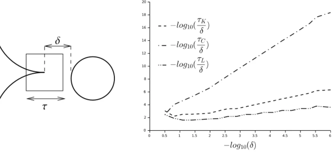
For a given parametric representation of a curve, PTOPO computes the special points on the curve, the characteristic box, the corresponding graph, and then it visualizes the

Vous pouvez aussi rejoindre l’un des nombreux GROUPES associés, ou le quitter si un ami vous y a inclus et qu’il ne vous convient pas (beaucoup l’ignorent, mais il est