Characterization of the dynamic response of continuous system discretized using finite element methods

Characterization of the Dynamic Response of

Continuous Systems Discretized Using Finite

Element Methods

by

Sandra Rugonyi

Nuclear Engineer, Balseiro Institute, Argentina (1995)

Master of Science in Mechanical Engineering, M.I.T. (1999)

Submitted to the Department of Mechanical Engineering

in partial fulfillment of the requirements for the degree of

Doctor of Philosophy in Mechanical Engineering

at the

MASSACHUSETTS INSTITUTE OF TECHNOLOGY

June

2001

ARCHIVES

@

Massachusetts Institute of Technology 2001. All rights reserved.

MASSACHUSETTS INSTITUTE OF TECHNOLOGY

JUL 1 6 2001

A uthor ...

... ....

..

LIBRA R IES

Department of Mechanical Engineering

May 25, 2001

C ertified by ...

..

...

Klaus-Jilrgen Bathe

Professor of Mechanical Engineeing

Thesis Supervisor

A ccepted by ...

...

Ain Ants Sonin

Chairman, Graduate Committee

Characterization of the Dynamic Response of Continuous

Systems Discretized Using Finite Element Methods

by

Sandra Rugonyi

Submitted to the Department of Mechanical Engineering on May 25, 2001, in partial fulfillment of the

requirements for the degree of

Doctor of Philosophy in Mechanical Engineering

Abstract

Nonlinear dynamic physical systems exhibit a rich variety of behaviors. In many cases, the system response is unstable, and the behavior may become unpredictable. Since an unstable or unpredictable response is usually undesirable in engineering practice, the stability characterization of a system's behavior becomes essential.

In this work, a numerical procedure to characterize the dynamic stability of con-tinuous solid media, discretized using finite element methods, is proposed. The pro-cedure is based on the calculation of the maximum Lyapunov characteristic exponent

(LCE), which provides information about the asymptotic stability of the system

re-sponse. The LCE is a measure of the average divergence or convergence of nearby trajectories in the system phase space, and a positive LCE indicates that the sys-tem asymptotic behavior is chaotic, or, in other words, asymptotically dynamically unstable. In addition, a local temporal stability indicator is proposed to reveal the presence of local dynamic instabilities in the response. Using the local stability indi-cator, dynamic instabilities can be captured shortly after they occur in a numerical calculation. The indicator can be obtained from the successive approximations of the response LCE calculated at each discretized time step. Both procedures can also be applied to fluid-structure interaction problems in which the analysis focuses on the behavior of the structural part.

The response of illustrative structural systems and fluid flow-structure interac-tion systems, in which the fluid is modeled using the Navier-Stokes equainterac-tions, was calculated. The systems considered present both stable and unstable behaviors, and their LCEs and local stability indicators were computed using the proposed proce-dures. The stability of the complex behaviors exhibited by the problems considered was properly captured by both approaches, confirming the validity of the procedures proposed in this work.

Thesis Supervisor: Klaus-Jiirgen Bathe Title: Professor of Mechanical Engineeing

Acknowledgments

Now that I have finished my graduate work at MIT, my mind goes back in time and I cannot regret the decision to come here. My memory is full of enriching experiences.

I remember moments of intense joy, and extremely stressful situations. This is the

life at MIT, full of contrasts. Needless to say that I could not have come so far if it were not for all the people that, in one way or another, were near me.

I would like to take this time to thank all the people that made this possible. I am

sure I will not include absolutely everyone in this acknowledgement, since otherwise the list will be extensive, but at least let me mention the people that had most influenced my life during this four years.

First of all I would like to express my deepest gratitude to Prof. Klaus-Jiirgen Bathe, my thesis advisor, who guided me through the world of research and could always find the way to challenge me. I truly enjoyed our fruitful discussions during the development of this research work, and I am grateful for his constant support and encouragement. I would also want to thank the members of my Thesis Committee, Prof. Carlos E. S. Cesnik and Prof. Ahmed F. Ghoniem, for their suggestions and encouragement during the development of my thesis.

I am very grateful to Prof. Eduardo Dvorkin for giving me the opportunity, when I was an inexperienced engineer, to explore the world of finite element methods and

for encouraging me to continue my studies at MIT. His advice and wise guidance during my "first steps" are invaluable to me.

This research has been partially supported by the Rocca Fellowship for which I am very grateful.

I would also like to thank the people of the Finite Element Research Group at MIT (my office-mates) Suvranu De, Nagi El-Abassi, Anca Ferent, Dena Hendriana, Jean-Frangois Hiller, Phill-Seung Lee, Daniel Pantuso, Juan Pablo Pontaza, Denise Poy and Ami Salomon for their encouragement and support, and for providing a friendly atmosphere in the "lab". We spent many afternoons discussing academic problems and sharing experiences that enriched me beyond expectations. In addition, I am

thankful to the researchers of ADINA R & D for their help and support with the use of ADINA. I would also like to thank Leslie Regan, from the Mechanical Engineering Department, for her patience, help and constant support, and for having always a big smile.

During this four years, the constant support of my friends, who always found the way to give me strength during difficult moments and with whom I shared many exciting experiences of my life, was invaluable. A big thank you to Emma Sanchez, Galit Toledo, Rita Toscano, Miguel Marioni and Debra Blanchard: without you I could not have made it.

I would like to express my gratitude to my parents, whose support and

encour-agement mean the most to me.

Finally, my utmost gratitude goes to Mauro, my husband and best friend, for his love and encouragement and for always showing me the light at the end of the tunnel and giving meaning to my life.

Contents

1 Introduction

2 Discrete dynamical systems

2.1 Nonlinear dynamic equations . . . . 2.2 Dynamic responses of nonlinear systems . . . . 2.2.1 Steady-state behavior . . . . 2.2.2 Periodic solutions . . . .

2.2.3 Chaotic behavior . . . .

2.3 Stability of motions: Lyapunov stability . . . . 2.4 Lyapunov characteristic exponents . . . .

2.4.1 Definition and properties of Lyapunov characteristic exponents 2.4.2 Numerical calculation of the maximum Lyapunov characteristic

exponent... ... 3 Governing equations of continuous media

3.1 Kinematics of continuous media . . . .

3.1.1 Lagrangian formulation . . . .

3.1.2 Eulerian formulation . . . .

3.1.3 Arbitrary Lagrangian-Eulerian formulation

3.2 Conservation equations . . . . 3.2.1 Mass conservation . . . . 3.2.2 Momentum conservation . . . . 3.3 Equations of motion . . . . 10 16 16 19 19 20 20 21 24 24 31 34 . . . . 35 . . . . 35 . . . . 36 . . . . 37 . . . . 38 . . . . 39 . . . . 39 . . . . 40

3.3.1 Structural equations . . . . 40

3.3.2 Fluid flow equations . . . . 42

3.3.3 Fluid flow-structural interface conditions . . . . 44

4 Finite element formulation 45 4.1 Structural equations . . . . 46

4.2 Fluid flow discretization . . . . 47

4.3 Fluid flow-structural interaction problems . . . . 52

5 Lyapunov characteristic exponents of continuous systems 61 5.1 Structural problems . . . . 64

5.2 Fluid problem s . . . . 77

5.3 Fluid-structure interaction problems . . . . 79

5.4 Local stability . . . . 80

6 Numerical examples 82 6.1 Discrete nondimensional equation of motion: the Duffing equation 82 6.2 Structural system s . . . . 92

6.2.1 Analysis of steady-state behavior . . . . 92

6.2.2 Buckled beam analysis . . . . 95

6.2.3 Beam subjected to nonlinear boundary condition . . . . 98

6.3 Fluid-structure interaction . . . . 101

6.3.1 Collapsible channel . . . . 102

6.3.2 Modified collapsible channel model . . . . 106

7 Conclusions and future work 114

List of Figures

2-1 Graphical representation of the different types of stability of a motion,

according to Lyapunov. . . . . 23

2-2 Graphical representation of the evolution of perturbations in all direc-tions in a two-dimensional phase space. The vectors ei and e2 change directions as the value of t increases. However, we are concerned with the basis vectors associated with t - 00. . . . . 27

3-1 Reference, spatial and mesh configurations. . . . . 36

4-1 9/3 elem ent. . . . . 50

4-2 General fluid-structure interaction problem. . . . . 53

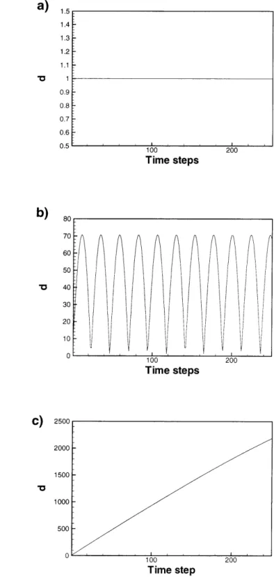
5-1 Numerical calculation of norm of the perturbation for the harmonic oscillator equation. The time step used in all three cases is At = 0.3. a) w = 1, b) w = 100, c) w = 5000. . . . . 72

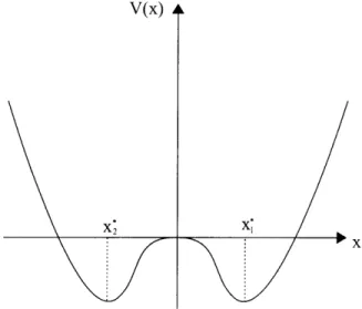
6-1 Sketch of the potential function of the Duffing equation without forcing and when all the parameters are positive numbers. . . . . 84

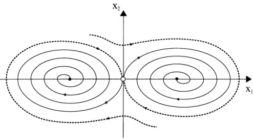
6-2 Sketch of the phase portrait for the Duffing equation without forc-ing. The black dots correspond to stable fixed points for the system, whereas the white dot (at the plot origin) corresponds to the unstable fixed point. . . . . 85

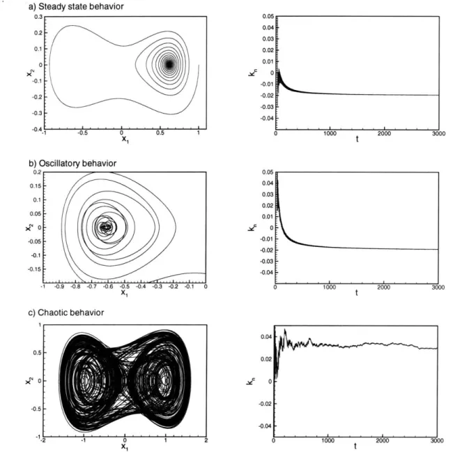
6-3 Different behaviors exhibit by the Duffing equation and the values of the LCEs associated with them. a) Steady-state response. b) Oscilla-tory behavior. c) Chaotic response. . . . . 88

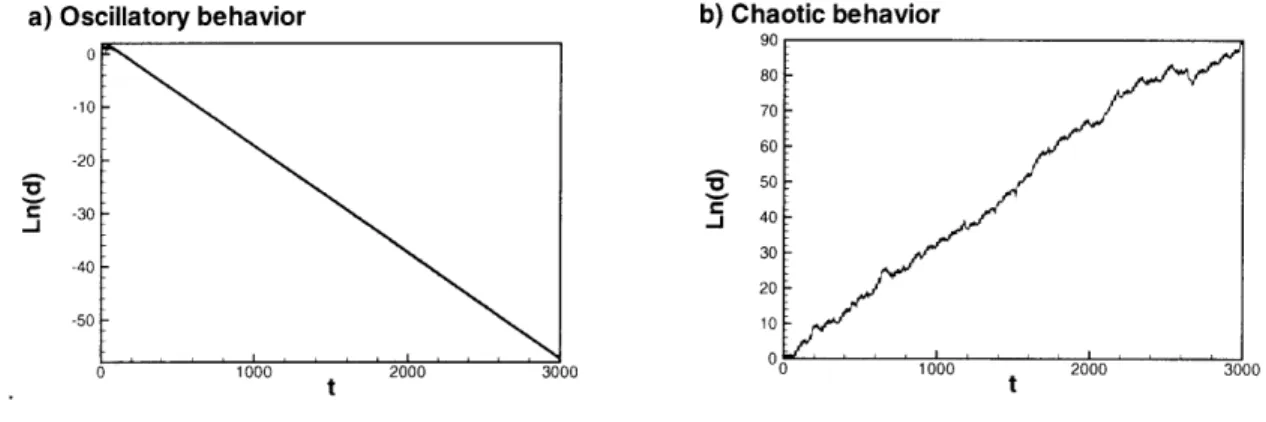
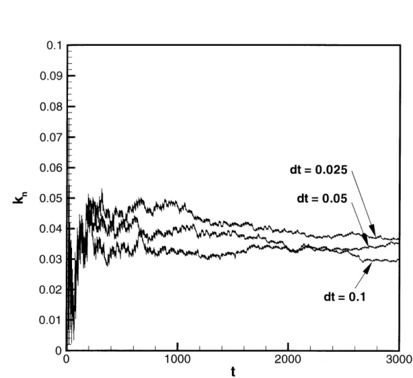
6-4 Values of ln(d) as a function of time for two responses of the Duffing equation. a) Oscillatory behavior. b) Chaotic response. . . . . 89 6-5 Values of k, obtained when the Duffing equation presents the chaotic

behavior considered above, and for different values of the time step used to discretize the equations in time. . . . . 90 6-6 Comparison of the values of k, obtained for the chaotic response of

the Duffing equation considered above, using the method proposed by Benettin et al. and the proposed procedure. . . . . 91 6-7 Cantilever beam used in the analysis of the perturbation evolution of

a steady-state behavior. . . . . 92 6-8 LCE calculation of a steady-state solution of the cantilever beam.

Os-cillation of the values of k, are typical when using the proposed pro-cedure (since the norm of the perturbation is calculated using only displacem ents). . . . . 94

6-9 Buckled beam problem considered. . . . . 96 6-10 Mid-point displacement of buckled beam problem and LCE calculation. 97 6-11 Fourier spectrum of the buckled beam response obtained for the

mid-point displacem ent. . . . . 97 6-12 Plot of In(d) as a function of time for the buckled beam problem. Note

that the local stability of the system is captured by this graph, without explicitly calculating the system LCE (which defines only the system long-term stability) . . . . 99 6-13 Convergence analysis for the LCE value obtained in the case of the

buckled beam . . . . 100

6-14 Beam subject to nonlinear boundary conditions. Sketch of system considered . . . . 100 6-15 Displacement of the end of the beam with an attached cubic spring

(the "free-end") as a function of time; and the calculated values of kn, which give the response LCE in the limit for time going to infinity. . 102

6-16 Fourier spectrum of the response obtained for the beam with an

at-tached cubic spring, shown in Figure 6-15. . . . . 103 6-17 Calculated in(d) as a function of time, for the beam problem with

nonlinear boundary conditions. . . . . 104

6-18 Collapsible channel problem considered . . . . 106 6-19 Mid-point displacement of the collapsible segment for the collapsible

channel problem depicted in figure 6-18, and the calculated LCE. . . 107

6-20 Plot of the ln(d) as a function of time for the collapsible channel problem. 108 6-21 Power spectrum of the mid-point collapsible segment displacement

ob-tained for the channel problem. . . . . 109 6-22 Modified collapsible channel problem considered. A parabolic velocity

profile, constant in time, is imposed at the tube inlet. The linear truss of constant k = EA acts over one point of the membrane when it

reaches a vertical displacement of 0.009m or more inside the channel, and it does not interfere with the fluid flow inside the channel. . . . . 110 6-23 Collapsible segment mid-point displacement for the channel problem

depicted in Figure 6-22, together with the calculated values of k,. . . 111 6-24 Power spectrum of the mid-point collapsible segment displcement

ob-tained for the modified channel problem. . . . . 112

6-25 Plot of ln(d) as a function of time for the modified channel problem. . 113

A-i Natural logarithm of the distance between two trajectories that were

originally very close to each other. The trajectories were calculated using the Duffing equation and for the value of parameters analyzed in Chapter 6 that result in a chaotic behavior. . . . . 120

Chapter 1

Introduction

The complexity and large variety of behaviors that nonlinear systems can exhibit have fascinated researchers for centuries. For many systems, even weak nonlineari-ties cannot be neglected since they significantly affect the long-term system response. Furthermore, analytical solutions are usually difficult or impossible to obtain, and con-sequently, techniques have been developed to approximate either the system response in time or its asymptotic behavior (usually when weak nonlinearities are present). Unfortunately, all these analytical techniques, although very useful, are only appli-cable to a relatively small number of systems due to the intrinsic complexities of them.

The availability of computers made possible the numerical calculation of the re-sponse of systems that were impossible or extremely difficult to solve by other means, and therefore it opened a broad spectrum of new possibilities. Furthermore, as the speed and storage capacity of computers increases, the calculation of more complex and larger systems becomes feasible. Numerical methods constitute nowadays an essential tool in the analysis and understanding of the behavior of systems, with applications in almost all areas of engineering and science.

Since the early inception of the analysis of mechanical systems, it was recognized that nonlinear systems, as opposed to their linear counterparts, exhibit a large variety of behaviors. It was then also acknowledged that the characterization of the system's response stability, not only of equilibrium points but also of motions, was important.

Thus, mathematical tools, such as perturbation methods, were developed to assess the stability of system behaviors. When using perturbation methods the system re-sponse is slightly perturbed and the evolution of the perturbations as a function of time solved (or approximated). Generally, if the perturbations decay as a function of time, the system dynamic behavior analyzed is stable, whereas if the perturbation grows in time, the response is unstable. Due to the complexity of the calculations involved, analytical techniques were limited to the study of relatively simple systems. Therefore, for the stability characterization of system's responses, computers are in-valuable tools for researchers and engineers in the study of large and complex systems. The objective of this work is to use numerical methods to characterize the stability of the dynamic response of continuous systems.

Let us begin with a brief description of what has been done in the area in the past.

By the end of the 19th century, mathematicians had noticed that certain dynamical

systems present irregular solutions. For those irregular solutions, small perturbations in the initial conditions lead to large differences in the system response at a later time, making prediction impossible. Nevertheless, it was believed and generally accepted that using powerful enough computers any deterministic system (i.e. a system that has no random inputs or parameters, and which is governed by a known equation of motion) could eventually be solved and its response predicted.

In the second half of the 20th century, Lorenz was computing trajectories of a very simple deterministic system he had developed with the aim of studying and predicting the weather. To his surprise, he found that for certain values of the parameters of his equations, irregular solutions exist [18]. The name chaotic behavior, to define the response of such trajectories, was then employed to describe this type of motions.

A chaotic behavior is characterized by a non-periodic response and sensitivity to

initial conditions. Nearby trajectories in phase space (the space of displacements and velocities in a classical mechanical system) diverge exponentially fast (on average) from each other, and the response becomes unpredictable.

Since the work of Lorenz, many researchers have studied the chaotic behavior of numerous low-order discrete equations of motion and maps. Furthermore, techniques

were developed to characterize a chaotic response by assessing how fast nearby trajec-tories in phase space diverge from each other. Such measures include the Lyapunov characteristic exponents of a system response and the Kolmogorov entropy (which can be calculated by knowing the Lyapunov characteristic exponents). Even though the concept of Lyapunov characteristic exponent was developed in 1892 by A. M. Lyapunov, the basis for its numerical calculation was only given in 1976 by Benettin et al. [4] [3].

In engineering practice, turbulence, a chaotic behavior of fluids, was known since long ago, and researchers have characterized and calculated it by means of statistical variables. It was also recognized that the exact system behavior is unpredictable in the presence of turbulence, since it is impossible to exactly trace the trajectory of a particle, no matter how much we try to avoid errors in the calculation. Although the dynamic behavior of a turbulent flow is unstable and unpredictable, its mixing characteristics are usually desired in engineering systems, for example to dissipate heat in a more efficient way.

However, the recognition that the response of solid mechanics problems as well as electrical systems can become chaotic was more surprising and somewhat unexpected. Especially surprising was the fact that nonlinear systems of equations with only a few degrees of freedom, obtained from Newton laws of motion, could exhibit a chaotic response. In contrast to fluid systems, in structural mechanics an unstable behavior is usually not desirable and hence the chaotic behavior unacceptable. Thus, the characterization of the dynamic stability of structural engineering systems becomes important.

Chaotic responses have been observed in diverse dynamical continuous systems, in-cluding buckled beams and arcs with periodic excitations, electro-mechanical systems, systems subject to nonlinear boundary conditions such as contact, pipes conveying fluid and fluid flow over plates, to mention just a few [24].

Previous works on the chaotic behavior of continuous systems include experimen-tal investigations and the use of reduction methods, see for example [25] [27] [16] [6]

recording some of the system variables as a function of time. Then, the time histories are analyzed using Fourier and correlation analyses and finally numerical techniques are applied (see for example [38]) to obtain an approximation of the response Lya-punov characteristic exponent. This approach, although powerful, is not available for every system since the costs of it might be unaffordable. In the case of reduction tech-niques, it is assumed that the system response is accurately described by considering the response of only a few system modes. The continuous equations that describe the system behavior are then reduced to a system of a few coupled discrete nonlin-ear equations, that can be analyzed using the available techniques for the analysis of discrete systems of equations. However, the amount of modes needed to accu-rately represent the system behavior is not always evident. Even worse, when strong nonlinearities are present, the linearized modes are no longer accurate to describe the system behavior, and nonlinear modes, which can be very difficult to obtain, should be employed. Therefore, reduction methods also present intrinsic limitations.

A more general procedure to assess the local stability and calculate the Lyapunov

characteristic exponent of a continuous system response is therefore needed.

It is important to emphasize here the main differences between systems of equa-tions obtained by discretizing a continuous system and discrete equaequa-tions of motion. The objective of this discussion is to explain why the numerical techniques developed to calculate the LCE of discrete systems could not be employed in the calculation of the LCE of continuous systems. The first difference is that when discretizing a con-tinuous medium using finite element methods, a large number of discrete equations is obtained. Another immediate difference is that the continuous problem boundary conditions have to be satisfied at all times. However, the most important difference is that distinct time scales are present in the continuum discretized equations. Usually the time step chosen to discretize the equations (when using an unconditionally stable time integration scheme) does not accurately capture the smaller time scales involved in the equations. From the discussion of Chapter 5, it becomes clear that the algo-rithm to calculate the LCE of discrete systems, describe in Chapter 2, is no longer applicable in the calculation the LCE of continuous systems, and a new procedure

needs to be developed.

In this work, a numerically efficient procedure to calculate the Lyapunov charac-teristic exponent of structural and fluid-structure interaction continuous systems is proposed. In the procedure presented here the continuous equations of motion are first discretized using the finite element method, and then the Lyapunov characteristic exponent of the system response is calculated, considering all the system discretized modes. As far as we know, this is the first work in which the Lyapunov charac-teristic exponent of continuous systems, discretized using finite element methods, is calculated by perturbing all the discretized modes (or degrees of freedom).

In many situations, it is not important to know the exact value of the Lyapunov characteristic exponent, which is a measure of the asymptotic divergence of trajecto-ries in phase space, but rather to know whether the dynamic response of the system is unstable at any time. In such situations, the characterization of the response local stability becomes very important and desirable. A local stability indicator, which can be obtained from successive approximations of the value of the Lyapunov char-acteristic exponent, is proposed to assess the local stability of the system response considered. These approximations are calculated at each time step in the LCE pro-cedure proposed, and therefore the local stability indicator can be thought of as a by-product of the Lyapunov characteristic exponent calculation.

The thesis is organized as follows. In Chapter 2 a brief review of the theory of discrete nonlinear dynamic systems is given, which includes the definition of the Lyapunov characteristic exponent and its numerical calculation. Chapter 3 is devoted to the continuum governing equations of solid media and fluid flows that are used in this work, as well as the conditions that must be satisfied at a fluid-structure interface when solving fluid-structure interaction problems. Chapter 4 describes the finite element discretization of those governing equations and the implementation of the fluid-structure interaction procedure employed. In Chapter 5, a numerically efficient algorithm to calculate the Lyapunov characteristic exponent of structural problem and of fluid-flows with structural interactions and a local stability indicator are proposed. Subsequently, in Chapter 6, numerical examples are presented and the

Lyapunov characteristic exponents calculated using the proposed algorithm. Finally, in Chapter 7 the conclusions of this work are given and future research in the analysis and characterization of the dynamic behavior of continuous systems is suggested.

Chapter 2

Discrete dynamical systems

Nonlinear dynamic systems can exhibit a large variety of dynamic responses, some of which are stable, and some unstable and unpredictable. Since instabilities in the system response are usually undesirable, it is not only important to calculate the response of the system but also to characterize its stability.

The objective of this work is to find numerical algorithms to characterize the stability of the dynamic behavior of nonlinear equations of motion, and to obtain information about the system response predictability.

In the following, a short introduction to some relevant aspects of nonlinear theory, needed for the development of this work, is given. For a more detailed explanation of the techniques available to study nonlinear systems and their responses, see for instance [37] [28] [8] [1].

2.1

Nonlinear dynamic equations

Consider the following system of discrete nonlinear non-dimensional ordinary differ-ential equations,

x = f(x) (2.1)

with initial conditions

x(to) = xa (2.2) where x C R" is the vector of state variables for the system, the dot indicates differ-entiation with respect to time, f is assumed to be a smooth vector valued function of x defined on some subset U C R" such that f : U * R", xa C U and to is the initial time. The system defined by equations (2.1) is called autonomous since the function f(x) does not depend explicitly on time.

When the function f is also a function of time, f = f(x, t), the system of equations is called non-autonomous. However, a non-autonomous system can be converted into an autonomous one. Assuming that x C R", by performing a change of variables of

the form xn+1 = t, equation (2.1) becomes,

x= f(x, xn+1) (2.3)

Jn+1

In this way, the time t is included as an additional state variable, and hence, all the techniques employed in the analysis of autonomous systems are also applicable to the non-autonomous ones.

The vector field f generates a flow

#t

#t

#(x,

function defined for all x

c

#t

d

Therefore,

#t

In addition,

#(xo,

[8].

by x,(t) for simplicity later in this work.

Let us define here, following

[8],

that if the distance between two points x and y is less than E, then y E S,. A set Sc is closed, if it contains all its limit points (or "boundary" points). A closed

and bounded set is a compact set. A p-dimensional manifold M C R (p < n) of a dynamical system is a set such that for each x belonging to the manifold there is a neighborhood Sm of x for which there is a smooth invertible mapping

#$:

The solution of equations (2.1) and (2.2) is unique, at least locally, if the existence

and uniqueness theorem [8] is satisfied:

Theorem 1: Let U C Rn be an open subset of the real Euclidean space, let f be a continuously differentiable (C) function in U and let xo E U; then, there is some constant c > 0 and a unique solution

#(xo,

satisfies equation (2.1) with initial conditions (2.2). o

Of course the theorem applies to all systems of equations that satisfy the theorem

conditions, and therefore unique solutions exist regardless of the dynamic stability of the system (i.e. it is applicable to responses such as steady-state solutions, periodic or quasi periodic solutions, chaotic behavior, etc.).

Theorem 1 is only local on time 1 since it can only guarantee the existence and uniqueness of solutions in some finite time interval (-c, c). The theorem becomes

global, and thus solutions exist for all times, if x is defined on a compact manifold M [8].

Theorem 2: Equation (2.1), with x E M, and f a continuously differentiable

(C') function, has solution curves defined for all t E R. o

Therefore, flows on spheres or tori, for example, are defined for all values of time, since the trajectories cannot escape from the mentioned manifolds.

In this work only deterministic systems, that is to say systems that contain no stochastic terms or inputs and whose equations of motions are known, will be con-sidered. In addition, only systems that satisfy the conditions of Theorem 1 and therefore have a unique solution,

#(xo,

be discussed.

The space of state variables x

C

'It is possible to find examples of equations defined in !R' for which solutions exist for all values

of t, but in general it is not possible to show the global existence in such cases without specifically

called the system phase space. Phase portraits, wich are plots of the trajectories in the phase space, are often used to analyze the response of nonlinear systems. The existence of unique solutions for the system of equations considered implies that trajectories never intersect in phase space.

An invariant set S for a flow

#t

#(x,

#(x,

#(x,

t -+ 00 for all x c A'. The subset of all points in which the system initial conditions

can lie so that the trajectories are attracted to the attracting set A is called the

domain of attraction or basin of attraction of A. Thus, all trajectories starting in the

domain of attraction of an attracting set are "captured" by the set. These concepts will be used in relation with the stability of motions and the chaotic behavior of systems. In this context, the attracting set of a chaotic system, observed numerically, will be called a strange attractor, although in theory there is some distinction between an attractor and an attracting set 2 (see

[8]

Given a nonlinear system of equations with specified initial conditions, our prob-lem is to find the reference solution and to determine its stability.

2.2

Dynamic responses of nonlinear systems

The solution of nonlinear equations of the form (2.1) with initial conditions (2.2) can present a rich variety of behaviors. Some of them are somewhat surprising and can only occur for nonlinear systems. Some of the behaviors that were observed in physical systems are mentioned below.

2.2.1

Steady-state behavior

A steady-state response can take place for both linear or nonlinear systems, and it

is obtained when x = 0 in equation (2.1). Thus, a steady-state response is obtained when the system reaches a state that does not depend on time, and therefore x is

2

a constant vector, also known as a fixed or equilibrium point of equations (2.1). In a dynamic solution, a (stable) steady-state response is obtained for large values of time, for dissipative systems, or when the initial conditions coincide with the system fixed point, for conservative systems.

2.2.2

Periodic solutions

Periodic solutions can be obtained for both linear and nonlinear systems. For con-servative systems (which can be linear or nonlinear), the amplitude of oscillations depends on the system initial conditions.

For nonlinear equations self-excited oscillations, also called limit cycles, can occur

[37]. A limit cycle is an isolated closed orbit in phase space, which can occur even

without imposing an external periodic forcing to the governing equations of motion. In other words, a limit cycle is a periodic solution, and neighboring trajectories are either attracted or repelled by the limit cycle (depending on the stability of it). In addition, for initial conditions lying in the basin of attraction of a limit cycle, the amplitude of the resulting self-excited oscillations does not depend on the system initial conditions.

2.2.3

Chaotic behavior

Among the different behaviors that a nonlinear system can exhibit, the chaotic re-sponse is one of the most intriguing ones. The most impressive characteristic is that an non-periodic random-like response (the chaotic response) can be obtained from a completely deterministic system, for which all the inputs are known. This is in contrast with the usual meaning of random system, in which a random response is observed because it is impossible to identify and control all the inputs to the system in an experimental setup.

A chaotic response is characterized by its sensitivity to initial conditions that

re-sults in an unpredictable behavior. Nearby trajectories in phase space diverge from each other exponentially fast. Therefore, two trajectories, which are initially

infinites-imally close to each other, are separated after a relatively short time, associated with

the prediction time of the system.

However, even when a chaotic response is observed, in the long-term, the trajec-tories occupy only a certain closed subset of the phase space, an attracting set called the strange attractor. All trajectories that originate close enough to this subset, in its domain of attraction, are attracted to it, in a similar way as trajectories that are close to a limit cycle are attracted to it. It can happen, for example, that for cer-tain initial conditions a nonlinear system is completely regular, and for instance the trajectories approach a fixed point (steady-state) as time evolves; whereas for other initial conditions the system behavior becomes chaotic. In addition, it is also possible to have a system with different chaotic attractors. Therefore, we refer to a chaotic

response of a system and not a chaotic system.

2.3

Stability of motions: Lyapunov stability

The concept of stability in physics can be applied to both equilibrium positions and

motions. In the first case, we consider solutions of equation (2.1) such that x = 0, and

therefore f(x) = 0. The zeroes of f(x) are called the system equilibrium positions or

fixed points. If the equilibrium is perturbed and the system returns (after certain time)

to the same equilibrium position, the equilibrium is said to be asymptotically stable, and stable (or neutrally stable)

[8]

In this work, we are concerned about the stability of motions. Therefore, we want to investigate what happens when a system that is not in an equilibrium position is perturbed. To characterize the stability of motions, the concept of Lyapunov stability can be used [10].

Considering equations (2.1) and (2.2), we now assume that the reference solution, Xr(t), which describes the system dynamic behavior, is slightly perturbed at time t, that is to say,

x(t) = x(t) + y(t) (2.5) where x is now the perturbed vector of state variables and y is the perturbation

vector, which is such that

||yl|

||xr||.

of the perturbation is given by

y

The stability of the reference trajectory can now be established by looking at the stability of the equilibrium point y = 0 of equation (2.6). Considering an initial perturbation yo at time t*, the Lyapunov stability is defined as follows [10],

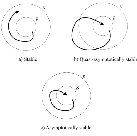
* The equilibrium is said to be stable if given two real numbers, E, 6, for each

E >0 there exists a 6 > 0 such that if ||yo| < 6 then ||y(t)|| < E for t > t.

" The equilibrium is said to be quasi-asymptotically stable if there exists a 6 _{> 0} such that if ||yoll < 6 then limto |ly(t)||= 0.

" The equilibrium is said to be asymptotically stable if it is both stable and

quasi-asymptotically stable.

" The equilibrium (y = 0), _{and therefore the motion considered, is unstable if it}

is not stable.

These concepts apply to the stability of a motion, and therefore it is possible to consider stable or unstable trajectories in phase space. For example, a trajectory that ends in a fixed point (i.e. a steady state solution) or in a limit cycle is stable, since trajectories that are initially close to each other converge to the fixed point or limit cycle orbit. However, a chaotic trajectory is unstable since nearby trajectories diverge from each other. A graphical representation of the different types of stability, according to Lyapunov, is shown in Figure 2-1.

Note that in the definition of quasi-asymptotic stability, the system is not neces-sarily stable at all times (it is only required for it to be stable for large times).

b) Quasi-asymptotically stable

c) Asymptotically stable

Figure 2-1: Graphical representation of the different types of stability of a motion, according to Lyapunov.

2.4

Lyapunov characteristic exponents

The Lyapunov characteristic exponents are used to characterize a system dynamic behavior, especially in the case in which a chaotic response is obtained. In this section, the definition and properties of Lyapunov characteristic exponents are considered, and the numerical calculation of the maximum Lyapunov characteristic exponent of order one briefly discussed (for discrete systems of equations of the form of equation (2.1)).

2.4.1

Definition and properties of Lyapunov characteristic

exponents

Consider the case of a nonlinear system of equations of the form (2.1), for which the function f generates a differentiable flow

#t

[3].

This problem is related to the asymptotic behavior of infinitesimal perturbations y(t) to a reference trajectory x,(t), solution of equations (2.1) and (2.2).

As discussed in Section 2.3, the equation that describes the evolution of pertur-bations is given by

f(x, + y) - f(x,) (2.7)

The above equation can be linearized (since the perturbation considered is infinitesi-mal), resulting in the following equation for the evolution of the perturbations,

)

=_y (2.8)

X=X

where ( f/0 x is the Jacobian matrix of the vector function f(x). In what follows it is assumed, for simplicity, that Cartesian coordinates are employed and therefore matrices instead of tensors will be defined and used. Of course, the same concepts are applicable when other coordinate systems are considered.

A solution of equation (2.8) exists and is unique for every initial condition, y(t*) = yo, if the Jacobian matrix of the function f(x) evaluated at x, satisfies the conditions of Theorem 1 at any time 3. It can be shown that if f(x) is continuously differentiable the conditions are satisfied. In such a case, the perturbation can be expressed by

(2.9)

where the matrix <b(t, t*) is the linearized flow matrix, a linear map of the tangent space of the vector function f(x,) at time to, Eo, onto the vector space associated with the tangent space of f(x,) at time t, Et. The following relations, for the mapping 4), are satisfied,

<b (t2, to*) = <b (t2,i ti) <b (tiI t*) <b(t, itn) = I

where t2 > ti > t*, and I is the identity matrix. Note that, since the matrix <b is

obtained from equation (2.8) and the Jacobian matrix changes as a function of time, <b depends on the specific times considered and on the reference trajectory chosen.

Assume that

1

lim -ln ||4(t, t*) < oc (2.11)

t-+oo t

where the norm of the matrix <b is usually defined as

||<bJ

conditions (2.2), is defined by

1 ||y(t) '|

X(YO, Xr) = lim sup - in (2.12)

t-+oo t ||yo||

where the supremum is taken since otherwise the function can be oscillatory and the limit not defined.

From equation (2.12) the following properties can be derived,

3_{Note here that to , the initial time for the perturbation, is not necessarily equal to to, the initial} time for the equations of motion.

ON

. Given a constant number c

X(C YO, Xr) X (YO, X,) (2.13)

Proof:

In|| cyll = In ||c|| + In lyl

and therefore property (2.13) follows from equation (2.12). o

" Given two perturbation vectors y1 and Y2,

X(Yio + Y20, X,) < max{ X(yio, x,), X(Y20, X,)} (2.14)

Proof:

Assume that

||Y1||

||Y2||,

In ||Y1 + Y2 1 In (1Yi 11 + ||Y2 ||)

" In [ 1y,1 (1 + flY211/fl1Yl

) I

" In ||y,1| + In (1 + ||Y2|| / 1|Y|)

Since Iy2

/|

/

and property (2.14) follows from equation (2.12). o

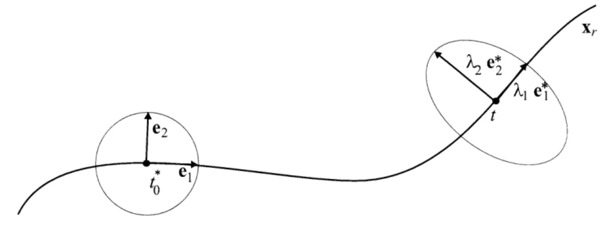
Suppose that we have an n-dimensional unit sphere D in the tangent space of

f(x) at x,(t*), Eo (we can think of D as an n-dimensional unit sphere of perturbed initial conditions). The image of D in the tangent space Et at x,(t) is given by the

the mapping <P(t, t*) and is in general an ellipsoid, see Figure 2-2. It is possible to associate each ellipsoid semiaxis with a coefficient of expansion (also called a Lyapunov characteristic number), Ai, in the direction of the image vector of the semiaxis in the

space E0. Furthermore, we can associate each coefficient of expansion with a Lyapunov

characteristic exponent, and therefore we have at most n Lyapunov characteristic

exponents, where n is the dimension of the tangent space: 1

Xi = lim sup - lnA with i = 1, 2,. . . , n. (2.15)

Xr

Figure 2-2: Graphical representation of the evolution of perturbations in all directions in a two-dimensional phase space. The vectors ei and e2 change directions as the

value of t increases. However, we are concerned with the basis vectors associated

with t -± oc.

The coefficients of expansion Ai correspond to the eigenvalues of the matrix (4 T)

(since the eigenvalues of 4 might be imaginary numbers).

A basis ei, e2, .. ., e, in !R, such that ||ei|| = 1 with i = 1, 2, . .. , n, is called

nor-mal by Lyapunov if E' x(ei, x,) is a minimum for the basis, and therefore the basis

{ej}

1

X(ei, x,) = lim sup- ln(Ai) (2.16)

t-*oo t

and therefore,

X(e, x,) = lim sup - In det < (2.17

i=1 t-+Oo 2t

Then, xi = x(ej, Xr), are the characteristic exponents associated with the basis vectors and they form the spectrum of Lyapunov characteristic exponents of first order (or one-dimensional). Arranging them in descending order,

It can be shown that if the reference trajectory does not end in a fixed point, the Lyapunov characteristic exponent of a vector tangent to the orbit of the flow is zero

[3] [11]. Therefore, except in the case of steady-state solutions, at least one of the

Lyapunov characteristic exponents of first order is zero.

When a normal basis is considered, property (2.14) becomes,

X(ei + e2 +- .. . + en, Xr) = max{ X(ei, x,), X(e2, Xr),... , X(en, Xr)} (2.19)

since the vectors ei are orthogonal.

Expressing the perturbation y as a linear combination of the normal basis defined above,

y = ciei + c2e2 + ... + cnen (2.20) where c1, c2, ... , cn are constants. Using properties (2.13) and (2.19) it follows that

X(YO, Xr) Xi (2.21)

except in the case in which yo has no components in the direction of the basis vec-tor ei associated with x1 (in a numerical calculation, however, round-off errors will always introduce a component in the mentioned direction). As a consequence, using equation (2.12), the maximum Lyapunov characteristic exponent, which will be de-noted simply as the Lyapunov characteristic exponent or LCE, is in general obtained (it is always obtained in a numerical calculation). An alternative explanation is ob-tained by considering equation (2.9). At each time step, y tends to grow more in the direction of the eigenvector of <b that corresponds to the eigenvalue with largest real part. As a consequence, after a sufficient amount of time the vector y would be aligned with the direction associated with X1, so that X1 would be obtained from the calculation. Therefore, the value of the LCE does not depend, in general, on the

initial perturbation vector selected, and thus X(yo, x,) = X(x,).

Since the LCE is a measure of the asymptotic divergence of nearby trajectories in phase space, all trajectories that start in the basin of attraction of an attracting set

will have the same LCE, and hence X(Xr) = Xi = X for all the trajectories considered that end in the same attracting set.

Let us also briefly consider here, for completeness, the so called k-dimensional Lyapunov characteristic exponents, although they are not used in this work.

Let gk c R' be a k-dimensional subspace generated by ei, e2, ... , e with k < n,

and Vk(t) the volume of the parallelotope determined by the vectors <b(t, t*) ei with

i 1, 2,. k. A k-dimensional Lyapunov characteristic exponent is defined by

X(k) (gk) = lim sup -In V(t) (2.22)

t-+oo t

Using the definition of the LCEs of first order,

X(k) (gk, X) - X(ei, xr) + X(e2, Xr) ... + X(ek, X,) (2.23) Choosing arbitrary vectors that span a k-dimensional space (such as in a numerical calculation), from properties (2.13) and (2.19) the largest values of the Lyapunov characteristic exponents of first order will be obtained,

X(k)(gk , Xr) = Xi - X2 + ... - Xk (2.24)

Therefore from the knowledge of the Lyapunov exponents of k-th order we can calculate the LCEs of first order. In fact, this property is used to calculate the complete spectrum of Lyapunov characteristic exponents of first order, see for example

[3] [7].

A natural question that arises is whether the exact LCE exists, that is to say,

whether the following number exists,

X = lim n

)

t-+oo t _||1yo||

This question was addressed by Oseledec in [30].

Assume that M is a smooth compact manifold on which the dynamical system of equations (2.1) is defined. If the flow

#t

at least one normalized invariant measure or probabilistic measure yu exists for the flow such that,

p(#(x, t)) p(X) (2.26)

p(M) 1 Then the Oseledec theorem [30] states:

Theorem 3: If a normalized measure pu(x) exists for the flow

#t

1 lim - In||<b(t, t*)| _(2.27) t-+oo t0 and therefore 1 /|y~t)| lm In

(O

exists for almost all x with respect to p if

sup

J

-dt<O<dt fm M

where ln+(a) = max{ln(a), 0}, with a E R. o

The Oseledec theorem is applicable to flows that are only almost everywhere differentiable. The fact that the limit exists for almost all x with respect to yu refers to the fact that there is a certain subset of the manifold M with measure zero, and then there exists a measurable set Mi C M such that p(M1) = 1.

Furthermore, Benettin et al [3] showed that if the flow

4t

4t

d(x,

exists a measurable subset Mi C M with I(M1) = 1 such that for every x E M1

2.4.2

Numerical calculation of the maximum Lyapunov

char-acteristic exponent

Let us consider again the nonlinear autonomous equations (2.1), with initial condi-tions (2.2), and the equacondi-tions that describe the evolution of perturbacondi-tions,

(

x=x, I(2.30)

y(t*) = Yo

where the initial times to and t* need not be the same, and in fact t* is usually chosen so that the system transient effects have decayed, since in this case the convergence to the LCE value in a numerical calculation is faster.

The basis for the numerical calculation of LCEs has been described in references [4] [3]. Both equations (2.1) and (2.30) have to be numerically integrated to calculate the systems reference solution and evolution of perturbations from which successive approximations to the trajectory LCE as a function of time are obtained. In the calculation of the LCE it is assumed that the system reference trajectory is "correctly" obtained, i.e. the system behavior is properly captured by the numerical discretization of the equations. See a discussion about numerical errors in [3].

In what follows, the procedure employed to calculate the maximum LCE of dis-crete dynamical systems is briefly described, following [3]. The procedure has been mainly used with non-dimensional first-order ordinary differential equations in time, consisting of only a few degrees of freedom.

Without loss of generality, we chose a random initial perturbation yo in equation

(2.30), such that yo 1, and a fixed time step At, so that t, = t* + nAt.

The time steps employed to numerically integrate the equations of motion (2.1) and the equations for the evolution of perturbations (2.30) need not be the same. However, it is convenient to use the same time step because the linearized matrices needed to calculate the evolution of perturbations are usually also employed in the solution of the equations of motion (when linearization is used in the solution proce-dure). Then, the coefficient matrices obtained after discretizing the equations in time are the same, and they need to be factorized only once and use in both the calculation

of the perturbation evolution and the system response. It is then especially conve-nient to use the same time step when large systems of equations, as those obtained when using finite element methods, are solved.

The evolution of the perturbation vector at each time step, t, can be calculated

by discretizing equation (2.30) in time and solving for y(t).

After n time steps the perturbation vector is 4

yn = Y (tn) = 4 (tn , t* ) yo = 41>(t, i n_1) 4(t _1 in2 .. (i t* y (231)

The perturbation vector Yn may grow (exponentially fast) if the behavior of the trajectory considered is chaotic. In such a case, an overflow of the computed vector would soon occur in a numerical calculation. To avoid the overflow, the perturbation vector is normalized at every time step (or after a certain number of time steps).

Considering the nth time step and

yn_1,

y*n = D(tn, in-1)

yn_1

and

dn = ||y*|| (2.33)

The obtained perturbation vector, y*, is then normalized to be used in the calcu-lation of the next time step,

y = (2.34)

dn

From equation (2.31), it is evident that following this procedure for n time steps,

||yn|| = dn dn_1 - - - di (2.35)

4

Here the matrices <b(tn, tn_1) are approximated discretizing equation (2.30) in time at each time step.

and an approximation to the LCE can be calculated at each time step as follows,

k=1 Iniyn||= E in(d.) (2.36)

n n i=1

The value of the LCE is calculated as the limit,

x = lim kn (2.37)

n -+oo, Atw

In practice, a good approximation to the value of the LCE is obtained when it

is observed that kn reaches a constant value as n is increased. Convergence to this constant value usually implies that a large number of time steps need to be calculated and therefore the evaluation of the LCE of a trajectory can be a time consuming calculation.

In summary, to calculate the maximum LCE of the trajectory of a nonlinear system, we start with a unit but otherwise arbitrary perturbation vector yo, such that ||yo|| = ||yOl = 1. Then, the following procedure is performed at each time step,

* Discretize the perturbation evolution equations in time and obtain y* from equation (2.32).

* Calculate the norm of the calculated vector y*, d, = ||y

,

* Normalize the perturbation y* to avoid overflow of the computed perturbation vector, equation (2.34).

* Calculate the approximation to the LCE, kn, from equation (2.36), and repeat the procedure for the next time step.

Chapter 3

Governing equations of continuous

media

The motion of continuous media is described by governing differential equations, which are derived from the laws of physics and constitutive equations.

Usually, the equations of motion of a solid medium are written using the

La-grangian formulation, i.e. the equations describe the position of particles as a

func-tion of time (with respect to a fixed frame), and therefore, particles are followed in their motion. In contrast, the fluid flow equations are usually written using the

Eule-rian formulation, i.e. the equations describe the fluid velocity and pressure at a fixed

spatial position. For fluid flow-structural interaction problems, a combination of both formulations, an arbitrary Lagrangian-Eulerian formulation, is required to describe

the fluid flow because the fluid domain changes as a function of time due to structural interactions.

In this chapter the Lagrangian, Eulerian and arbitrary Lagrangian-Eulerian for-mulations of motion are briefly discussed. The governing equations of Newtonian fluid flows and elastic isotropic solids are considered. In addition, the equilibrium and com-patibility conditions that must be satisfied at the fluid flow-structural interface are given.

3.1

Kinematics of continuous media

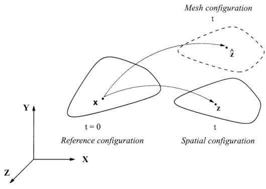
Consider a body (or a part of it) that is moving through space. The space occupied

by the body at time t = 0 is called the reference configuration, and the space occupied by the body at time t is called the spatial configuration (see figure 3-1).

At time t = 0 we can identify each particle of the body with a reference coordinate x. At time t the particle will be at a different position z. In other words, z is the position at time t of the particle that was at x at time t = 0.

There are different ways of describing the motion of the body (see, for example, [22]). Three of them will be considered here,

" Lagrangian formulation

" Eulerian formulation

" Arbitrary Lagrangian-Eulerian (ALE) formulation

Equations of motion are generally written in terms of material or physical particles. For example, when we say that a fluid is incompressible we mean that a particle cannot change its density with time, but different particles can have different densities. Newton's law of motion states that the rate of change of momentum of a body is equal to the sum of the external forces applied to that body, i.e. the law applies over a group of particles (that constitute the body) that are followed as a function of time. In general, when solving a dynamic problem using finite element methods, any of the above descriptions can be employed (see

[2],

3.1.1

Lagrangian formulation

In the Lagrangian formulation, the body particles are identified in the reference con-figuration, at time t = 0, and their movement followed as a function of time. The variables used to describe the equations of motion are then x and t. This descrip-tion is usually employed to describe the modescrip-tion of solids, for which the reference configuration is known.

Mesh configuration t

z

t=0 t

Reference configuration Spatial configuration

X

Figure 3-1: Reference, spatial and mesh configurations.

We are interested in deriving the Eulerian and ALE formulations from the La-grangian formulation, for different equations of motion. In particular, the time deriva-tives that appear in the equations of motion need to be transformed, see for example

[22].

3.1.2

Eulerian formulation

In the Eulerian formulation, the variables used in the description of the motion are z and t. The movement is described at a fixed spatial position z. The position occupied at t = 0 by the particle that is at z at time t is not important and usually not known. This description is generally used to describe the motion of a fluid flow.

At time t the position of the particles can be expressed as a function of the particle position in the reference configuration

z = ep(x, t) (3.1)

If equation (3.1) is known, then the velocity of a particle can be calculated by