Buckling patterns on pre-stretched bilayer shells

Buckling Patterns on Pre-stretched Bilayer Shells

by

Rashed Abdulazeez Al-Rashed

B.S., Massachusetts Institute of Technology (2015)

Submitted to the Department of Mechanical Engineering

in partial fulfillment of the requirements for the degree of

Master of Science in Mechanical Engineering

at the

MASSACHUSETTS INSTITUTE OF TECHNOLOGY

September 2017

@

Massachusetts Institute of Technology 2017.

S

Author..

Certified by.

I

All rights reserved.

ignature redacted

7

KiK-

~

D4parfirment of Mechanical Engineering

I

Pedro M. Reis

Associate Professor of Mechanical Engineering and Civil and

Environmental Engineering

Thesis Supervisor

Signature redacted

Accepted by ...

...

Rohan Abeyaratne

Professor of Mechanical Engineering

Chairman, Department Committee on Graduate Theses

JI

August 18, 2017

Signature redacted

MASSACHUSETTS INSTITUTE OF TECHNOLOGY

SEP 2 2 2017

Buckling Patterns on Pre-stretched Bilayer Shells

by

Rashed Abdulazeez Al-Rashed

Submitted to the Department of Mechanical Engineering on August 18, 2017, in partial fulfillment of the

requirements for the degree of

Master of Science in Mechanical Engineering

Abstract

We introduce a new experimental system to study the effects of pre-stretch on the buckling patterns that emerge from the biaxial compression of elastomeric bilayer shells. After fabricating our samples, releasing the pre-stretch in the substrate by deflation places the outer film in a state of biaxial compression and yields a variety of buckling patterns. We systematically explore the parameter space by varying the pre-stretch of the substrate and the ratio of film stiffness to substrate stiffness. The phase diagram of the system exhibits a variety of buckling patterns: from the classic periodic wrinkle to creases, folds, and high aspect ratio ridges. Our system is capable of easily transitioning between these buckling patterns, a first for biaxial systems. We focus on the wrinkle to ridge transition, where we find that pre-stretch plays an essential role in ridge formation, and that the ridge geometry (width, height) remains approximately constant throughout the process. For the localized ridge patterns, we find that the propagation of the ridge tip depends strongly on both strain and stiffness ratio, in a way that is akin to hierarchical fracture of brittle coatings.

Thesis Supervisor: Pedro M. Reis

Title: Associate Professor of Mechanical Engineering and Civil and Environmental Engineering

Acknowledgments

I would like to thank my advisor, Professor Pedro Reis, for his constant help and guidance. His direction and support has shaped my growth over the past two years. To Francisco L6pez Jim6nez, thank you for your mentoring, wisdom, and inhuman pa-tience while I learned the ropes. To the rest of EGS.Lab, thank you for the welcoming and supportive environment.

Warmest love and thanks to my family for their continued support, without whom none of this would have been possible. You are an inspiration.

Contents

1 Introduction 9

1.1 M otivation . . . . 9

1.2 Wrinkles, creases, and folds . . . . 12

1.3 Ridges: History and state of the art . . . . 14

1.3.1 Literature review of ridges . . . . 14

1.3.2 Ridges in relation to other surface patterns . . . . 18

1.4 O utline of thesis . . . . 20

2 Experimental Apparatus and Protocol 21 2.1 Overview of the sample fabrication protocol . . . . 22

2.1.1 Substrate fabrication . . . . 22

2.1.2 Initial system setup and pressurization . . . . 23

2.1.3 Pouring and curing of the film layer . . . . 24

2.1.4 System deflation and video capture . . . . 25

2.2 Characterizing the mechanical properties of the bilayer system . . . . 26

2.2.1 Stress profile of the hemispherical bulge . . . . 27

2.2.2 Shear stiffness of the elastomer materials used for fabrication . 30 2.2.3 Film layer thickness . . . . 31

2.2.4 Range of parameters explored . . . . 32

2.3 _{O utlook . . . .} 33

3 Results 35 3.1 Phase diagram - pattern classification . . . . 36

3.2 Critical film strain for pattern onset . . . .

3.3 Quantification of the geometry of ridges . . . .

3.4 Ridges onset and propagation . . . . 3.4.1 Propagation speed of the ridges . . . .

3.5 Structural hierarchy of ridge patterns . . . .

3.5.1 Limitations of our analysis . . . .

4 Conclusion

4.1 Summary of findings . . . . 4.2 Future work and potential applications . . . . 4.2.1 Ridge propagation and fracture . . . .

4.2.2 Translucency of pre-stretched bilayer systems

39 42 . . . . 46 . . . . 47 . . . . 50 . . . . 52 55 . . . . 55 . . . . 56 . . . . 56 . . . . 57

Chapter 1

Introduction

1.1

Motivation

Self-organized surface patterning in both natural and engineered systems can often appear as a buckling instability mode of a compressed thin stiff film bonded to a relatively thick compliant foundation [1, 2]. Such surface patterning often appears in nature, spanning a wide range of length scales. This is the case, for example, with intestinal organs, where surface instabilities appear as a result of the volumetric growth of the organ walls. Extensive surface instability along organ walls is connected to diseases such as inflammation, lymphoma, and asthma

[3].

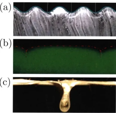
In the context of biofilms, surface wrinkling resulting from the maturation of certain species of bacteria is thought to act as a defense mechanism against antimicrobial agents [4].

When the film layer of a bilayer system is subjected to a sufficient amount of compressive strain, for example through constrained film swelling [51, bilayer com-pression [6], or substrate pre-stretch [7], the bilayer system can become unstable. Some representative examples of surface instabilities across different length scales in nature can be seen in Fig. 1-1. At a microscopic level, Fig. 1-la shows surface pattern-ing through bucklpattern-ing of a white blood cell membrane, which allows the membrane to expand when necessary [8]. Fig. 1-lb shows an example of naturally occurring surface patterning, where the skin of a grape wrinkles upon drying. Lastly, Fig. 1-1c shows a primate brain, where the irregular folded surface, greatly increases the functional

surface area of the brain [2].

(

₁₎

()(b

_0

Figure 1-1: Examples of surface instabilities in nature. a) White blood cell (adapted from Ref. [8]). b) Raisin (personal photo). c) Primate brain (adapted from Ref. [2]).

Historically, the prevailing intent surrounding bilayer system buckling has been to study them with the goal of preventing a potential failure mode. Efforts to rationalize the buckling of such bilayers date as far back as work done by Allen in 1969 [91, where two dense, stiff, and thin sheets of material are separated by a thicker, less dense, and more compliant material. The goal was to use sandwich panels as a structural unit, which meant buckling was studied as a failure mode and was scrutinized to be avoided. This narrative has extended across the years, with examples of more recent studies of bilayer bucking modes as a failure method coming through the lens of material coatings [101. Thin-film deposition is ubiquitous as a manufacturing method, often

used for material surface strengthening or as a thermal barrier. For example, optical polymers provide a lighter and more malleable material than glass in the automotive and optical industries but suffer from low surface hardness and sensitivity to various chemicals, including hydrocarbons [10]. Surface coatings can mask the weaknesses of optical polymers, so long as their integrity is not compromised. Compressive strains on such materials could lead to surface wrinkling

[6],

which can result in delamination of the surface coating, resulting in system damage or failure.

There has been a recent shift in perspective to focus on leveraging such surface instabilities in engineering applications. For example, surface patterning has been shown to be effective at preventing biofouling, with the change in the surface profile disrupting the growth of unwanted biological material [11]. Being able to change surface topography Vn demand has its other uses, such as smart adhesion, where controllable surface wrinkling resulting from the compression of bilayer systems can greatly enhance adhesion 112]. Recent studies have shown that surface wrinkling can drastically change the contact and roll-off angle of water droplets on gold film coated elastomeric materials, resulting in tunable wettability [13, 14]. Being able to change the surface profile on demand allows one to control the regime of the fluid in the boundary layer surrounding the surface (between laminar and turbulent), resulting in aerodynamic drag control [15, 16]. Surface wrinkling has also been shown to provide an inexpensive form of fabrication for microlens arrays

[17].

In order to fully exploit the potential of bilayer systems, significant effort has been devoted towards categorizing and quantifying the wide range of patterns available [18, 19], which range from patterns of wrinkles [20, 21, 22 and creases [23, 24] to more localized phenomena such as ridges [25, 26, 7] and folds [27, 6, 28]. These buckling patterns will be described in detail in Sections 1.2 and 1.3.

A large part of the experimental exploration of buckling modes have been done

in uniformly flat conditions, and pre-stretch is commonly applied only in a single direction, with biaxial loading conditions being less common [7, 29, 30]. Additionally, while periodic wrinkling and creasing have been studied for decades [9, 23], other sur-face patterns, such as the localized ridge buckling mode, have only been discovered

recently, and therefore remain relatively unexplored. Experimental systems where the primary parameters can be explored in detail can help alleviate the lack of un-derstanding of the underlying mechanics.

In the context of bilayer systems, there are certain parameters that govern buckling behavior [31, 18, 32]. These include the strain in the system, c, both in the film layer

Ef and the substrate layer E, and the pre-stretch, A0, of the substrate before film

adherence. We also consider the stiffness ratio of the two layers, ' = Af /As, where pf and p, are the shear moduli of the film and substrate layer respectively, in addition to the thickness of the film layer, tf. Typically, in such bilayer systems, the film layer is much thinner than the substrate layer, to the point where the substrate layer can be considered semi-infinite, resulting in its thickness being neglected from analysis regarding bilayer systems. Finally, we identify adhesion energy per unit area F, as a measure of the surface adhesion between the two layers.

What follows is a brief overview of the various buckling modes explored in the thesis, followed by a more thorough exploration of known literature on the ridge buckling mode, on which the majority of the thesis will focus.

1.2

Wrinkles, creases, and folds

Wrinkles are a periodic, continuous and non-localized buckling mode, sinusoidal in nature. As the oldest known and most scrutinized buckling mode, wrinkles have been studied for decades [9, 33, 34, 35]. Unlike most other buckling patterns, wrinkles are continuous, with no sharp variation in stress along the surface profile [36, 37]. The relative simplicity of wrinkles lends itself well to linear analysis in a way that does not extend to other, more localized forms of surface patterning [38]. A representative example of surface wrinkling can be seen in Fig. 1-2a.

Creases, in contrast to wrinkles, are a surface level, inwards facing buckling pat-tern where the surface buckles and comes into self-contact. Whereas wrinkles are periodic and continuous, creases are a localized mode, characterized by their sharp tips, as seen in Fig. 1-2b. One of the earliest forays into creases comes from Biot's

(a)

(b)

(c)

Figure 1-2: Figure showing cross sectional views of: (a) wrinkles (adapted from Ref. [39]; (b) creases (adapted from Ref.

124]);

and (c) folds (adapted from Ref.

161).

work on the instabilities of rubber under compression [231. Biot predicted the critical strain necessary to observe creasing, c, _{= 0.46. This was later found to be}

incon-sistent with experimental results, where creasing was observed at a critical strain of c, = 0.35, much earlier than previously predicted [40]. More recently, detailed

analysis by Hohlfeld and Mahadevan has lead to the more accurate prediction of

EC = _{0.354 [2, 41], a prediction that was later supported by experimental results [42].}

Biot's analysis of creasing conditions was purely linear, and the consideration of non-linearity led to predictions that more closely agree with experimental data

143,

44]. The sharp tips that are characteristic to a crease are what render linear analysis in-sufficient [45]. Creases have been observed as a result of compressive strains applied to a homogeneous soft material, in addition to the bilayer systems which are the focus of this thesis [241.

com-pression to a bilayer system that initially experiences wrinkling [25]. Folds are similar to creases in that they are a localized buckling pattern that warps inwards with re-spect to the surface of the bilayer system [46]. The distinction between the two buckling modes is most easily seen when comparing the cross-sectional view of the two, such as in Fig. 1-2b and c. While we can easily observe a sharp discontinuity in Fig. 1-2b, Fig. 1-2c is wider, deeper, and continuous. Folds lack the characteristic sharp tip observed in creases [47]. The wrinkle to fold transition has been extensively studied [28, 39], and folds have been observed as a result of soft bilayer composites in addition to thin stiff films resting on liquids [6].

1.3

Ridges: History and state of the art

A ridge is a high amplitude strain localization that appears when compressive strain

is applied to a bilayer system past the onset of wrinkling when specific conditions are met

[48].

If the substrate is exposed to a sufficient amount of pre-stretch, A0, before

film adherence, ridges can emerge. Ridges are the most recent buckling pattern to be discovered, with the earliest mention of ridges in the literature dating to 2012 [25].

1.3.1

Literature review of ridges

Cao and Hutchinson [25], in their seminal 2012 study, computationally explored the results of applying compressive strains on bilayer systems. The study was motivated

by a lack of understanding of post-bifurcation buckling modes. In particular, they

refer to Biot's earlier study of bilayer systems and note its lack of consideration of certain crucial situations, such as the case where both layers are jointly compressed, or when the substrate is pre-stretched. While exploring known advanced buckling modes such as period doubling and folding through simulation of two Neo-Hookean layers, the introduction of sufficient pre-stretch led to a sharp, outwards facing localization, which they termed the "mountain ridge" mode or ridge for short. They predicted that a threshold value of pre-stretch was required for the appearance of ridges. Their simulations showed that a pre-stretch of AO = 1.3 did not result in the emergence of

ridges, while AO = 2 did.

Nearly simultaneously, work by Ebata and Crosby [22] experimentally demon-strated the existence of the ridge buckling mode. These authors ran bilayer experi-ments with the goal of exploring the transition from wrinkling to strain localizations such as delamination and folds. These experiments were performed using polystyrene

(PS) films on Polydimethylsiloxane (PDMS) with a pre-stretch of AO = 1.1. The

polystyrene was spun-cast to vary the film thickness (5 to 180nm, compared to a substrate thickness of 4 mm). The substrate was pre-stretched using a uniaxial strain stage, after which the film was transferred to the PDMS substrate via a water bath. They reported finding "folds with an outward morphology," which were later classified as ridges. It is worth noting that, in this study, ridges were observed at

AO = 1.1, a much lower value of pre-stretch than the previously predicted lower limit

of Ao = 1.4 [7, 48]. To date, there is no explanation for this discrepancy.

Later in 2012, Zang and Hutchinson presented the first targeted study of ridges, both experimentally and computationally [26]. Their simulations suggested that

AO = 1.4 is the minimum required pre-stretch for ridges to appear. Experiments

were run using PDMS for the substrate, utilizing a plasma treatment to form a thin stiff film along the surface. The film thickness varied between 10 and 20 nm, com-pared to a substrate thickness of 1mm, with a stiffness ratio of = 1.56 between

the film and substrate layers. Despite testing up to a pre-stretch of AO = 1.5, they

could not experimentally witness ridge formation. The authors did, however, witness localization. They additionally established that pre-stretch produces softening for outward displacements, and hardening for inward displacements, which helps explain why ridges only appear with the introduction of pre-stretch into the system. The fact that Zang et al. did not observe ridge formation despite crossing the predicted (and later verified [71) required pre-stretch for ridges could be due to both the substrate and the film being comprised of the same silicon-based polymer. Similar effects have been observed with Vinyl Polysiloxane (VPS), another silicon-based polymer, by Pez-zula and Holmes

[49],

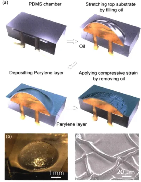
where differing amounts of free polymer chains led to relative swelling.

Further work by Takei and Hutchinson [7] explored ridges formed under biaxial pre-stretch. A layer of PDMS was bulged using an oil chamber, giving it a known pre-stretch. A thin layer of Parylene-C was then deposited on the pre-stretched PDMS substrate, as seen in Fig. 1-3a. The removal of said pre-stretch led to the observance of wrinkling, followed by ridge formation. The study included predictions on ridge geometry such as ridge width and height resulting from FEM simulations, which correlated loosely with the experimental data presented. Similar experimental biaxial exploration of ridge formation was simultaneously done by Cao and Zhao

1131,

imposing biaxial pre-stretch on a planar system. In their experiments, uniaxial or biaxial pre-stretch was applied to an elastomer film, after which a gold film was sputter-coated onto the substrate. Most notably, the two directions of pre-stretch were relaxed at different independent rates. In some tests, they released the pre-stretch at a uniform speed biaxially. In others, they relaxed the pre-stretch in one direction completely, before relaxing the remaining pre-stretch. The difference between the two was visible in images taken of the fully relaxed system. Sequential relaxation led to ordered ridges with a clear directionality, while simultaneous relaxation led to disordered, seemingly directionless ridges.

The most thorough exploration of the wrinkle to ridge transition comes through computational and experimental work done in 2015 by Jin and Hutchinson

[48].

By

modeling the two layers as Neo-Hookean and running numerous two-dimensional plane strain simulations, they explored the wrinkle to ridge transition in addition to the subsequent return from ridges to wrinkles as the compressive strains are removed from the system. When cycling between the two states, a distinct hysteresis response was observed: the critical strain at which wrinkles transitioned to ridges was distinct from the critical strain at which ridges reverted to wrinkles. For example, for a pre-stretch value of AO = 2 and a stiffness ratio of = 1000, wrinkles would transition

to ridges at approximately w- = 0.036, while the reverse transition would happen

at Er = 0.023. They proceeded to note that the wrinkle to ridge transition in this

regime is unstable, the consequence of which is that wrinkles will rapidly snap into ridges, provided sufficient pre-stretch (Ao = _{1.4). These results are corroborated by}

PDMS chamber Stretching top substrate

by filling oil

Oil

Depositting Parylene layer Applying compressive strain by removing oil

4e.h

Parylene layer

Figure 1-3: Figure showing a method of biaxial exploration of ridges. (a) Schematic showing the pre-stretched bilayer fabrication process. (b) Image of the experimental setup in its pre-stretched state. (c) Image detailing the ridge structure, as taken through an SEM. Figure adapted from work done by Takei and Hutchinson [7].

experiments where a stiff, thin layer of PDMS is deposited onto a softer, thicker, uniaxially pre-stretched layer of PDMS. The film and substrate thickness were tf = 7.3 pm and tf = 500 pm, respectively, with stiffness ratio = 77 and pre-stretch A =

2. The experiments showed an observable hysteresis effect, which agreed qualitatively with earlier simulation results.

1.3.2

Ridges in relation to other surface patterns

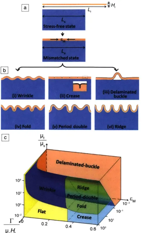
Work done by Wang and Zhao [31, 18, 32] has helped put ridges into the broader context of previously known buckling modes. After studying bilayer systems subject to uniaxial pre-stretch, they developed and presented a three-dimensional phase di-agram highlighting the conditions under which they observed a number of distinct buckling modes, including wrinkles, creases, delaminated buckles, folds, ridges, and period doubling, as seen in Fig. 1-4b. The phase diagram itself, as seen in Fig. 1-4b,

is presented as a function of stiffness ratio (, mismatch strain EM, and normalized

adhesion energy . The stiffness ratio ( = g represents the relative stiffness of

p, Hf u

both layers of the bilayer system, where pUf and ps are the shear stiffnesses of the film and substrate respectively. The mismatch strain Em = _{Lfrersnstedfeec}-Ls represents the difference

in strain between the two layers, where Lf and L, are the length of the film and sub-strate layers respectively. Normalized adhesion energy is a measure of how bonded the two layers are, signified by the adhesion energy per unit area IF, normalized by the stiffness of the substrate M, and the thickness of the film layer Hf.

Such characterization is ongoing, with recent work by Zhao et al.

119]

involving sur-faces with distinct curvature, both concave and convex, in an effort to quantitatively distinguish between buckling patterns. They first engaged in theoretical analysis of a two-dimensional slice of a tubular bilayer structure, noting the differences between their curved system and the flat, planar systems typically studied. Both concave and convex geometries were explored by alternating the placement of the film layer between the outwards and inwards surfaces. Fast Fourier Transform (FFT) analysis was used to distinguish between wrinkles, creases, folds, ridges, and period doubling. Wrinkling, for example, results in a regular, sinusoidal wave, and therefore only has one frequency detected by FFT. Patterns such as creasing are much more irregular, leading to a wide range of frequencies detected by FFT. They find that concave struc-tures prefer creases and folds, while convex strucstruc-tures prefer ridges. This is the first quantitative measure used to differentiate between the various buckling modes in any context; a significant feat.

4

L

Stress-free state Mismatched state, (b) Delaminated 1) Crease buckle

(v) Period double (vi) Ridge

P PS I s'Otudde

7id

Ridge 1010 10* -0 1 ouat 10-1 10Crease ₁₀

r

0.2 0.4 0.6 103

Figure 1-4: (a) schematic showing a process by which to apply pre-stretch to a bilayer system. (b) the resulting buckling patterns observed. (c) Phase diagram of the patterns resulting from the experimental procedure shown in (a), as a function of

stiffness ratio = _SFLf L, mismatch strain Em = Lf-Ls, and normalized adhesion energy_{and or[ ideo2n.}

g8

fFigure adapted from work done by Wang and Zhao [18,

321.

Hf

b]

(I)Wrinkle (Iv) Fold JL T

Most of the current literature on ridges, particularly the wrinkle to ridge transi-tion, studies ridges in a simple context: two-dimensionally, with uniaxial pre-stretch. Additionally, phase diagrams presented that put ridges into context with the other known buckling patterns all also rely on uniaxial pre-stretch. The work presented in this thesis attempts to address both of these gaps of knowledge. We first aim to explore the parameter space of bilayer systems under biaxial pre-stretch, varying both stiffness ratio and pre-stretch A0 to provide a phase diagram complementing

uniaxial phase diagrams [31]. We then target the wrinkle to ridge transition, utilizing the uniquely larger scale of our system (ridge size on the order of 1 mm, where most studies involve ridges on the order of 1 pm) to illuminate the underlying mechanics.

1.4

Outline of thesis

In this introduction, we have provided an overview of the various buckling patterns and included the necessary background for the rest of the thesis. Chapter 2 details the experimental apparatus used to perform our tests, along with the corresponding experimental methods used to explore the parameter space. In Chapter 3, we relay our findings, presenting both the phase diagram resulting from exploration of our parameter space, as well as the results of our investigations into the wrinkle to ridge transition. We study the geometry of the ridges over the course of the deflation pro-cess, measuring both ridge width and height. We then investigate ridge propagation speed and ridge hierarchy, where the response of our system is reminiscent of fracture. Finally, in Chapter 4, we summarize the outcomes of the thesis and outline areas of future work.

Chapter 2

Experimental Apparatus and

Protocol

In this chapter, we describe the protocol to fabricate the samples used in our experi-ments, alongside the experimental setup and methods used to test said samples. We developed a fabrication method to consistently create elastomeric bilayer structures with a known pre-stretch AO, where we could readily tune the relevant system param-eters (pre-stretch and stiffness ratio). We designed and constructed an experimental setup with which we could obtain video data on the pattern formation process. Fi-nally, we describe the process followed to measure the relevant system parameters: the stretch A across the surface of the hemispherical bulge (including the initial pre-stretch AO), the shear modulus ft of all materials used, and the film thickness tf. To measure stretch A, we use a set of cameras to track the relative change in distance between markers placed along the surface of the hemispherical bulge. A set of uni-axial tension experiments is used to determine shear modulus p. Film thickness tf is determined through the use of an optical microscope.

2.1

Overview of the sample fabrication protocol

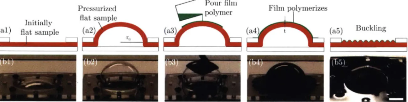
In Fig. 2-1a, we present a schematic diagram showing the sequential steps of the ex-perimental protocol that we followed to fabricate our bilayer samples. Photographs of the corresponding experiments are provided in Fig. 2-1b. First, a thick elastomeric disk was fabricated to be subsequently used as the substrate of the bilayer system. This disk was hydraulically inflated from its initially flat configuration to a nearly hemispherical shape, thereby setting a prescribed pre-stretch. A second liquid elas-tomeric polymer was then poured onto the now bulged substrate, which, upon curing, results in a thin shell that was bound to the bulged pre-stretched substrate. The sys-tem was then slowly deflated, and, as the pre-stretch was released, the film buckled to accommodate the excess in surface area. The following sections will detail each of these steps of the process, including tests done to measure the appropriate material properties when relevant.

Pressurized Pour film Film polymerizes

Initially flat sample

polymer

(al) flat sample (a2) (a3) (a4) t (a5) Buckling

Figure 2-1: (a) Schematic diagrams of the protocol followed to fabricate samples, with

(b) accompanying images to each corresponding step of the experiments. Samples

were fabricated by first, (1) clamping the foundation layer (elastic disk) between two acrylic plates, (2) pressurizing the system to pre-stretch the disk and achieve a nearly hemispherical shape, (3) pouring a liquid polymer onto the foundation layer which then (4) polymerizes into a thin shell coating. After depressurizing the system, (5) buckling modes are observed on the surface of the bilayer. The scale bar represents 2 cm.

2.1.1

Substrate fabrication

For the substrate of the bilayer system, we used flat disks of Polydimethylsiloxane (PDMS, Sylgard 184, Dow Corning), with a radius of R = 38 mm and a thickness

of H = 3.25 0.15 mm. This shape was chosen due to its lack of corners and ease

of fabrication. Acrylic molds were made through use of rapid prototyping techniques (laser cutting). The PDMS base and curing agent were then mixed at a specific ratio depending on the desired stiffness. Ratios of {20: 1, 22.5: 1, 25: 1} were used, resulting in a range of shear moduli p = {105, 156, 191} kPa. The values of As were determined from independent uniaxial tensile tests (5943, Instron) of dog bone specimens, the specifics of which will be detailed in Section 2.2.2.

After determining the appropriate amount of base and curing agent by weight, the mixture was then stirred thoroughly by hand for 2 minutes, followed by use of a centrifugal mixer (ARE-310, Thinky). This mixture was then poured into the prepared molds. The pouring process introduces significant amounts of air bubbles into the PDMS mixture, and therefore each sample was placed in a vacuum chamber for 30 minutes. Each sample was then inspected visually, at which point any remaining air bubbles and visible particulates were removed. Samples were then placed in a

convection oven at T = 1000 C for 10 hours.

2.1.2

Initial system setup and pressurization

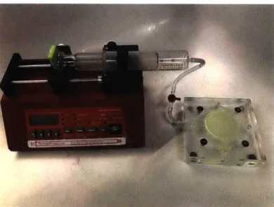
Once the PDMS disks were made, the substrate was then clamped in between two acrylic plates, ensuring that the ensemble was leak proof (Figs. 2-lal,bl). The lower acrylic plate had a smaller through hole where silicon tubing was mounted, which itself was then connected to a syringe pump (New Era Pump Systems NE-1000). The top clamping acrylic plate contained a circular cut out hole of radius r" = 25.4 mm, through which the PDMS samples eventually protrude (Figs. 2-lal,bl). This setup can be seen in Fig. 2-2. Water was then injected into the sample at a constant rate, at a sufficiently slow rate to ensure no entrapment of air, up to a maximum prescribed volume, Vm,. Tests were conducted to insure that no water permeated through the PDMS substrate on the timescale of our experiments (approximately 1 hour from pressurization to data gathering), eliminating a potential inaccuracy in our determined Vm, over time.

Figure 2-2: Photograph of the experimental setup used to pressurize and depressurize the bilayer system. A syringe pump is connected to an acrylic enclosure through silicon tubing. The syringe pump allows fine control over the inflation rate.

into a nearly spherical cap [50] (Fig. 2-1a2, b2). The radius and subtended angle of the bulge can be precisely controlled by varying the injected volume, Vmax, thereby allowing control over the amount of pre-stretch AO imposed on the substrate. Details on evaluating the stress state of the bulged substrate can be found in Section 2.2.1.

2.1.3

Pouring and curing of the film layer

After fixing Vmax, and therefore setting the pre-stretch of the bulged substrate, a second silicone-based liquid polymer, Vinyl Polysiloxane (VPS, Elite, Zhermack), was used to form the film layer. VPS base and curing agent were combined at a 1:1 ratio

by weight, after which a centrifugal mixer (ARE-310, Thinky) was used for mixing.

The VPS mixture was then poured onto the now nearly spherical bulged substrate (Figs. 2-1a3,b3). Upon curing, the VPS formed a thin polymeric shell that was stress-free in its original configuration. This thin shell had almost uniform thickness, set by the balance between viscous draining along the substrate and curing time for VPS

[51]

tf ~ , (2.1)

29Tc

,a i; I , Z' M

where Ao is the characteristic viscosity of the VPS prior to curing, R is the radius of the mold, p is the density, g is acceleration due to gravity, and rc, is the characteristic curing time. We note that the final thickness of the shell, tf, can be systematically tuned by delaying the time between the initial mixing of the polymer and the moment of pouring, while taking advantage of the fact that the viscosity of the polymer changes as the curing progresses, as shown previously by Lee et al.

[51].

After pouring, the VPS layer was left to cure at room temperature (T = 200 C), for 1 hour. By using different polymers (Elite Double 8, 16 fast, 22, and 32; Zhermack), we were able to systematically select a variety of shear moduli, [if = {75, 110, 194, 327} kPa, and

film thicknesses tf {220 7.8, 277 20, 271 13, 226 9} pm. Details concerning

both of these sets of properties can be found in Sections 2.2.2 and 2.2.3. It is important to highlight that throughout the curing process, the stress-free film is chemically bonded to the bulged substrate (which is pre-stretched), such that no delamination occurs during the experiments.

2.1.4

System deflation and video capture

After curing of the VPS film (Fig. 2-1a4), the water was then withdrawn using a syringe pump at either dV/dt = 15mL/min or 1 mL/min, both of which were slow enough for the unloading to be assumed as quasi-static. These deflation speeds cor-respond to an approximate (de)stretch rate of either dA/dt = -0.41 0.02 min-1 or

-0.027 0.001 min-1, respectively. Varying dA/dt had no observable effect on the

resulting type of buckling mode, nor on the characteristic size of the resulting pattern. The unloading progressively relaxes the pre-stretch of the substrate, while simulta-neously placing the film in a state of compression, which leads to the emergence of a variety of surface-buckling patterns of complex topography.

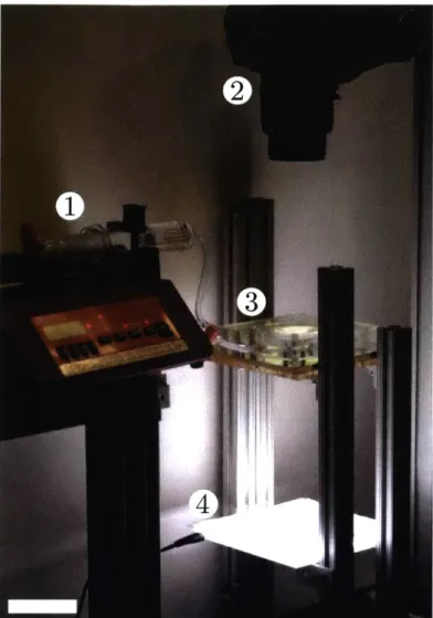
To best capture the pattern formation process, we built the experimental setup shown in Fig. 2-3. Samples were imaged by a digital SLR camera (Nikon D3200, Fig. 3,2) mounted perpendicularly to and above the hemispherical sample (Fig.

2-3,3), with the samples oriented upside down to shield the camera from potential

Figure 2-3: (a) Photograph of the experimental apparatus used to capture the pattern formation, including: (1) syringe pump, (2) camera, (3) bilayer specimen, (4) light source. Scale bar at bottom left indicates 10 cm.

a resolution of 1920 x 1080 pixels. These videos were then used to classify the different type of surface buckling patterns and quantify both the characteristic length and rate of propagation of the patterns.

2.2

Characterizing the mechanical properties of the

bilayer system

In the following section, we detail the methods used to measure the relevant mechan-ical properties of the system. We first detail a series of tests used to determine the

stretch profile of the hemispherical bulge across all levels of inflation tested. The goal of this process is to calibrate between the volume of water injected into the system, V, and the stretch, A, at any given point during the deflation process. We then describe a set of uniaxial tension tests to determine the shear modulus, p, of all the materials used in our experiments. Finally, we show the methodology used to measure film thickness, tf.

2.2.1

Stress profile of the hemispherical bulge

Stretch is a measure of deformation defined as the ratio between initial and final

(i.e., deformed) length, A = Lf/Li. Given the symmetry of our problem, the three

principal stretches are in the azimuthal, Aop, hoop, A0, and through the thickness,

AZZ, directions. A calibration between the extent of inflation as set by the volume

of injected water, V, and the stretch of bulged substrate disks was performed using the apparatus detailed in Section 2.1.2. Our technique provided data on two of the principal stretches, azimuthal and hoop stretch. Assuming full incompressibility of the PDMS substrate, the through the thickness stretch can be calculated as Azz = 1/(AOOAoo).

The calibration process consisted of using ink markers placed in concentric rings along the originally flat substrate, with initial radii ri = {2.7, 5.6, 8.5, 11.5} mm, see

Fig. 2-4b. Each of the four rings contained 3 markers. The system was then steadily pressurized, while two digital SLR cameras (Nikon D3200) were set perpendicularly to track the three-dimensional positions of the ink markers, as seen in Fig. 2-4a. The hoop stretch corresponds to stretching of each of the rings, and so for the j-th marker was calculated as Ai9 = rj/rj. The azimuthal stretch corresponds to stretching

between consecutive rings, calculated as

d (rj" r )

A3 = 'f (2.2)

(rj+l - rj)'

where d(r}f, r}) is the distance along the azimuthal arclength between the rings. In order to find the arclength used to calculate azimuthal stretch, images such as

S(b)

*(c)

4, Li 1 22 ? * A. X4 AA~ 1

A.1

₀

_A0

0 10 20 30 40 50 60

Volume injected, V [mL]

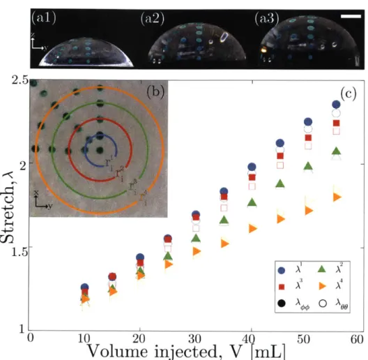
Figure 2-4: (a) Set of photos showing the process by which stretch is correlated to the volume of water injected, with the three images correlating to inflation levels of of V = 25, 40, and 55mL respectively, from left to right. Scale bar represents

10 mm. (b) top-down view of the sample in (a), along with a schematic showing the

location of the markers used to measure stretch before inflation. The first point ro lies at the center of the substrate, with ra = 2.7 mm, rb = 5.6 mm, r. = 8.5 mm, and

rd = 11.5 mm. (c) Correlation between amount of water injected into the system, V, and the resulting stretch, A, for the range of 10 < V < 55 mL. Stretch A is defined as the change between radii compared to the original radii shown in (b) Closed symbols refer to azimuthal stretch Ap, and open symbols to hoop stretch A0,.

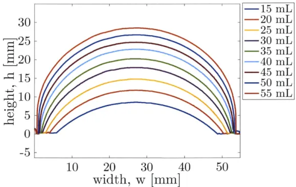
the ones shown in Fig. 2-4a were thresholded. These thresholded images were then used to extract the hemispherical profile at various levels of inflation. The results of this process can be seen in Fig. 2-5, where the side profile of the hemispherical bulge is shown for inflation levels in the range 15 < V < 55 mL. When combined with images taken from a top-down view (as in Fig. 2-4b), this allows us to find the arclength between any two markers.

The measured stretch at varying levels of inflation for the first four inner rings, spanning half the radius of the substrate, is shown in Fig. 2-4c. The data shown is the average of two independent experiments, using three markers per ring. The stretching decreases as the markers move away from the center of the bulge. The relationship between A00 and A0 also depends on the position, changing from purely

biaxial at the center, due to symmetry, to uniaxial at the boundary, where A00 = 0

due to the imposed boundary conditions. However, the stretching remains very close to biaxial in a large section of the substrate. In particular, the difference between the two principal stretches at the four points measured never exceeds 5%.

-15

mL

30-

-20

mL

-25

mL

-25-

-30

mL

-35

mL

20 -

_-40

_mL

15

--

_-50

45 mL

_mL

4iD

-

55 mL

00 5

0

-5 r

10

20

30

40

50

width, w [mm]

Figure 2-5: Graph showing the hemispherical profile of the pre-stretched system, as the injected volume is varied. Note that our experiments vary between 25 mL and 55 mL.

Hereon, the azimuthal stretch at the pole of the bulged substrate will be used to define the stretch of the system. Consequently, the range of explored pre-stretch is

1.5 < A. < 2.4, which corresponds to an injected volume of water within the range 25 Vmax [mL] < 55.

2.2.2

Shear stiffness of the elastomer materials used for

fabri-cation

To evaluate the shear modulus of both PDMS and VPS, we run uniaxial tension tests on dogbone-shaped samples of all varieties of materials used in the experiments: three different mixtures of PDMS {20: 1, 22.5: 1, 25: 1}, and four different types of VPS (VPS8, VPS16, VPS22, and VPS32). The dogbone specimens were fabricated in acrylic molds as described in Section 2.1.1. Each dogbone was marked with two black lines before being mounted in the Instron. The dogbone was then tensioned with a digital SLR camera (Nikon D3200) recording the process.

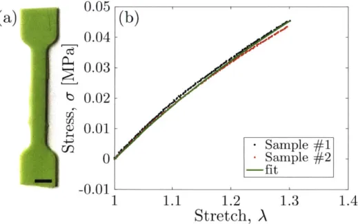
Through image processing analysis (MATLAB) of the resulting videos, we ex-tracted data on stretch A = L/Li as a function of time. By combining this data with the Instron's provided data of force as a function of time, and factoring in the dimensions of the dogbone itself, we obtain the data presented in Fig 2-6b.

(a)

0.05 (b)

0.04

0.03

S0.02

9 0.01 - Sample #1 0 - Sample #2 -fit -0.01 1

1.1

1.2

1.3

1.4

Stretch, A

Figure 2-6: (a) Example of a VPS32 dogbone specimen used for uniaxial testing. Scale bar represents 10 mm. (b) stress as a function of stretch from a test run for PDMS mixed at a ratio of 25:1 involving 2 dogbones. The resulting Neo-Hookean fit, represented by the solid line, was used to extract the shear modulus A.

We rely on a Neo-Hookean model to describe the non-linear elastic response of the two elastomeric materials used

[521.

For an incompressible Neo-Hookean solid,

we can compute the strain energy

W = 2(A 2 + A2 + A 2 -3).

2 1 2 3 (2.3)

Incompressibility also means that AjA₂A3 = 1. In the case of uniaxial stretch, A, = A,

and therefore A₂ = A3 =

,

meaning the strain energy can be written as

W= A(A2 +2 3).

2 A (2.4)

Taking the derivative of the strain energy results in stress

dW 1

dA A2). (2.5)

Given the data presented in Fig 2-6b, we can then fit for the shear modulus A. Each stiffness value is the result of two testing runs, each run involving 2 or 3 specimens, the results of which are seen in Table 2.2.2.

Table 2.1: Shear modulus of relevant materials.

Polymer type P PDMS 25:1 105 PDMS 22.5:1 156 PDMS 20:1 191 VPS 32 327 VPS 22 194 VPS 16 110 VPS 8 75

2.2.3

Film layer thickness

While the substrate thickness was comparatively easy to determine, as the disks were fabricated first, the film thickness tf is more difficult to compute. Please refer to Section 2.1.3 for more details on the film fabrication. In order to measure the film thickness, a bilayer sample was first fabricated as per standard procedure described

in Section 2.1. A slice was then cut from the bilayer system, roughly 2 mm by 1 mm in size, as close as possible to the peak of the hemispherical bulge. The film layer was then gently peeled from the substrate. After removal, the film layer was smooth, suggesting no residual strain in the film layer, which would potentially affect the thickness measurements. If there was any residual substrate attached to the film layer, or if there was any visible imperfection, the sample was discarded at this stage. Samples were then cut in half carefully, in order to have a smooth edge to measure.

Prepared samples were then put under an optical microscope (Nikon Optiphot), as seen in Fig. 2-7a. Resulting images were processed in image processing software (ImageJ), from which film thickness was extracted. Three images were taken for each film sample, and three measurements were taken for each image (9 measurements total per data point). Samples were fabricated at all tested levels of inflation, with all four film variations used (VPS8, VPS16, VPS22, and VPS32). The results of these tests can be seen in Fig. 2-7b, where we present film thickness tf as a function of pre-stretch Ao for different types of VPS. For all of the tests in this section, the substrate was PDMS mixed at a 1:25 ratio.

For each VPS type, one set of tests was run where multiple layers of film were formed. After the first film layer cured as usual, another layer of VPS was poured in the same fashion. The resulting experimental set had a sample with one pour, two pours, three pours, and four pours. It was found in all cases that the thickness of a sample with more than one pour was simply an integer multiple of the base thickness (within 2%). The only significant variance in thickness came from the difference in thickness between VPS types, as seen in Fig. 2-7b. The resulting film thicknesses used for VPS8, VPS16, VPS22, and VPS32 are tf = 220 7.8 pm, 277 20 pm,

271 13 pm, and 226 9 pm, respectively.

2.2.4

Range of parameters explored

By tracking the relative distance of markers as the system is pressurized, we obtain

information on the stretch A state along the surface of the hemispherical surface. Through a set of uniaxial tension experiments performed on dogbone specimens, we

3 5 0_r

)b)

-- 4vPS8

(b)

vPSI6

... VPS22 -VPS32 0 0 250 -14 OF 200-V.4 1.6 1.8 2 2.2 2.4 2.6 Prestretch ,A.

Figure 2-7: (a) Representative photograph of film layer taken from which thickness measurements are performed. The sample shown is VPS22, extracted from a sample inflated at A0 = 2.36. (b) Thickness of the film layer obtained after pouring VPS

onto substrates of varying values of pre-stretch. The horizontal lines represent the average thicknesses obtained from each polymer: VPS8, VPS16, VPS22, and VPS32 as t = 220 7.8 pm, 277 20 pm, 271 + 13 [im, and 226 9 pm, respectively.

determine the shear moduli of the various substrate and film layers used. Combined, these tests determine our explored parameter range. In obtaining the results presented in Chapter 3, we have varied pre-stretch A between 1.5 < A0 < 2.4, and stiffness ratio = - between 0.4< < <3.1.

's

2.3

Outlook

In this chapter, we presented the procedure by which we fabricate bilayer systems with a known, prescribed pre-stretch A0. We then detailed the experimental setup

used to obtain video data on pattern formation. In Chapter 3, we will see the results obtained by analyzing the experimental video data, show the variety of buckling patterns observed, and scrutinize the wrinkle to ridge transition.

33

-Chapter 3

Results

In this chapter, we present the results of the systematic exploration of the parameter

space using the methodology described in Chapter 2. We first present a phase diagram

highlighting the buckling patterns observed in a biaxial system as a function of varying

stiffness mismatch and pre-stretch A0. From the gathered video data, we identify

the critical strain of pattern formation and compare it to previously found theoretical

and experimental values. Shifting focus to the ridge buckling mode, we study the

wrinkle to ridge transition in particular. We use 3D laser scanning techniques to

measure the geometry of the ridge (height and width). The ridge propagation speed

was measured from video data and studied over a variety of conditions, exhibiting

behavior reminiscent of fracture. Finally, the system is studied as a whole to comment

3.1

Phase diagram

-

pattern classification

In Fig. 3-1, we present a phase diagram, including representative examples, of the variety of buckling patterns observed during the deflation of our bilayer samples. The pattern classification was performed by qualitative inspection of the obtained buck-ling modes. Our results show that the two primary parameters of the system are the prescribed pre-stretch, A0, and the stiffness ratio between the film and the substrate, = [f//ls. This is in agreement with the existing literature for uniaxial

stretch-ing [181. Our systematic exploration of the (A0, ) parameter space has identified the

following distinct patterns: wrinkles (Fig. 3-la), ridges (Fig. 3-1b), hierarchical ridges (Fig. 3-1c), creases (Fig. 3-1d), and folds (Fig. 3-le). The phase diagram presented can be split into two main regions based on whether the stiffness ratio is above or below unity. When the film is stiffer than the substrate ( > 1), we observe wrinkles,

ridges, and hierarchical ridges, i.e., buckling modes that tend to protrude outwards from the surface. When the film is softer than the substrate ( < 1), patterns of

creases and folds are observed instead, both of which are directed inwards from the surface.

Let us first focus on the regime where the stiffness ratio is above unity, ( > 1.

Wrinkles [20, 21, 22] (Fig. 3-ia) are observed for high stiffness ratios and low values

of the pre-stretch (observed in our system at 1.55 < Ao < 1.83 and 1.02 < < 3.1). These wrinkling patterns correspond to a periodic, continuous and non-localized

buckling mode, without the sharp changes in height exhibited in the other observed patterns. Periodic ridges [7, 25, 26] (Fig. 3-1b) are obtained for higher values of the stiffness ratio and pre-stretch: 1.7 < A0 < 1.83 and 1.49 < < 3.1. These ridge

patterns correspond to high aspect ratio and localized protrusions from the polymer surface. Further increasing pre-stretch (1.91 < Ao < 2.36 and 1.02 < K < 3.1),

yields hierarchical ridges (Fig. 3-1c), which differ from periodic ridges primarily in their method of onset. Within the periodic ridge regime, large sections of ridges tend to appear simultaneously. By contrast, hierarchical ridges appear individually and sequentially, with each ridge 'tip' nucleating suddenly and then propagating until the

U

I P% I % a.V.ZA -We L)~~ IN WOO 2 Pre-stretch, A 0 2.5

Figure 3-1: Phase diagram of the rameter space of pre-stretch, A0, a

different buckling patterns observed in the pa-nd stiffness ratio, : a) Wrinkles, b) Ridges, c) Hierarchical Ridges, d) Creases, and e) Folds. No surface patterns are observed in the region marked with the left-facing triangles (<). The top row of images shows typical examples of the partially formed patterns (Ef = 0.3 0.04). The bottom row represents the fully established patterns (Ef = 0.36 0.06). Darker regions within the pattern images represent areas of sharp change in height. Scale bar represents 5 mm.

3 2 Q. CI) S A A A A A * * A A A A *A A A A A

-UA

A

A

A

A

SA A A A 1 1.5 'tg 4 W

ridge has fully formed. This behavior is reminiscent of a crack tip propagating on a brittle thin-film coating

[53].

An analogy between these localized ridge patterns and fracture will be explored in more detail towards the end of this chapter.

When the stiffness ratio is below unity, < 1, patterns of creases and folds form.

Creases [5, 23, 54] (Fig. 3-1d) are a surface-level buckling mode involving smaller

localized perturbations directed inwards with respect to the surface, appearing at low values of pre-stretch (1.55 < A,, < 2.13 and 0.4 < < 0.7). A crease exhibits higher

local strains when compared to the rest of the surface and has a sharp tip, in contrast to wrinkles, which are characterized by a continuous surface and even strain across the film. Folds [6, 27, 28] (Fig. 3-le) are obtained at higher values of pre-stretch

(2.13 < A. < 2.36 and 0.4 < < 0.7). Folds are a self-contacting buckling mode

that is directed inwards, into the substrate, similar in nature to creases. The most distinguishing characteristic of folds is their tendency to penetrate into the surface and the lack of the sharp tip that creases exhibit. At the lowest combination of stiffness ratio and pre-stretch (1.55 < A,, < 1.70 and = 0.4), no buckling mode was observed, and the surface of the samples remained smooth through deflation.

It is important to note that the transitions between the various regions in the phase diagram of Fig. 3-1 are not necessarily sharp, particularly when the pre-stretch the parameter that is varied. For example, at low values of stiffness ratio and moderate pre-stretch (e.g., Ao = 2.1 when transitioning from creases to folds), the observed patterns exhibit hybrid characteristics of both sides of the phase boundary. The transition between buckling modes is sharper when the stiffness ratio is varied. As such, the phase diagram presented should be regarded more as a guiding map for the relative location of the various patterns.

Similar phase diagrams have been produced in systems where the patterns result from uniaxial stretching or compression [181, which show good qualitative agreement with our results. In the case of biaxial stretching, however, previous experimental studies have focused on a single pattern, such as wrinkles

[551,

folds

[281,

or ridges

17].

To the best of our knowledge, our experimental system is the first to exhibit all of these buckling patterns, albeit in different regions of the parameter space.

3.2

Critical film strain for pattern onset

Next, we quantify the conditions for the onset of the buckling patterns in our bilayer samples during deflation. After obtaining an extensive set of video data through the process described in Sec. 2.1.4, each video was used to identify the critical strain

c, = 1 - A,, where A, is the stretching of the film at the pattern onset. This was done

by first identifying the approximate location of first pattern appearance in the video,

followed by a more thorough examination of the frames surrounding the pattern onset until a frame is chosen. This procedure was repeated for all the samples represented in Fig. 3-1.

Fig. 3-2 shows the critical strain experienced by the film at which each specific pattern is first observed, c, as a function of stiffness ratio, , and for different values of pre-stretch, A,. The presented data can again be separated into two regions, with a boundary at a stiffness ratio of unity. The most immediate observation is the apparent lack of dependence of c, on A0. In contrast, the critical film strain does exhibit some

dependence on .

At a stiffness ratio below unity

((

< 1), where we observe creases and folds, we

first compare our data to classical predictions set forth by Biot in 1963 [23], where he posited a critical strain of Ec = _{0.456. Biot's initial analysis was purely linear, however,} and did not take into account the sharp corners that are prevalent in creases. More recent nonlinear analysis and simulations

[2]

have lead to an updated prediction of

EC = 0.354

[56],

which is in moderately good agreement with the experimental data presented in Fig. 3-2.

On the other hand, when the stiffness ratio is above unity

((

> 1), we observe

wrinkles, ridges, and folds. We now compare our data to a power-law description put forth by Wang et al. _{[18], obtained through an energetic scaling argument,}

Ec = a -3, (3.1)

which has been supported by experimental data in the range 1.3 < ' < 16, with

0.3I K -

-K>

0.2

I-O

Creases Folds 0 1 0 0 1 0.5 0.4 2 Stiffness ratio, ( 3 4

Figure 3-2: Graph showing the critical strain experienced by the film C at which buckling patterns are first observed, as a function of stiffness ratio , at various amounts of pre-stretch A,. Creases and folds are represented by hollow symbols at a stiffness ratio below unity, while wrinkles, ridges, and hierarchical ridges are represented by full symbols.

al. [18] determined the phase boundaries by setting Hi = H3, where li and HF are the potential energies of the patterns being compared. This was performed while keeping all other parameters constant, which in their study includes stiffness ratio L= , mismatch strain Em = Lf -L, and normalized adhesion energy r (please

1AS Lf /-Lsf

refer to Sec. 1.3.2 for more details). The potential energy H of a bilayer system is defined as N = Uf + U, + FD, where Uf and U, are strain energies per unit width of

the film and substrate, respectively, and rD is the adhesion energy of the two layers multiplied by the delaminated length of substrate. After the computation of these phase boundaries, they proceeded to verify their predictions experimentally.

A ==1.83

0

-Wang [2014]

=1.98 ... _{Adjusted Wang Fit}

. .4 A =2.13_{'.0 1} --- _{Biot [1963]} A0=2.25 _{- Hohlfeld [2011]} A A =2.36 ~ A

-4-Wrinkles

Ridges Hierarchical Ridges ;-- 4-0.1 1

It is difficult for us to make a clear statement on the functional form of our experimental data, vis-A-vis Eq. (3.1), due to its limited dynamic range. However, after fitting the prefactor of Eq. (3.1) to our data, a2 = 0.29 0.04, we find moderately good agreement. We speculate that the difference in the value of prefactor a from the study of Wang et al. [18] and our experiments could be primarily due to the difference in loading of the two studies (uniaxial and biaxial, respectively).

To verify the data obtained manually, FFT analysis was performed on a large sub-set of the videos analyzed. The difference between the manual and computationally found values for critical strain c, is shown in Fig. 3-3, calculated as

Z C (3.2)

where 0" is the critical strain found through FFT analysis, and Em is the manually found critical strain.

10 5 --3 * o -i ₀ 0 .0 r 5 -* ( =3.1 * ( =1.85 * ( =1.05 ( = 0.70 -10 1.5 2 2.5 Pre-stretch, A

Figure 3-3: Graph showing the deviation in critical strain between critical strain calculated manually and through FFT analysis (' and Ec respectively), calculated as A = ! _CM . The deviation is not found to be more than 5%.