Evaluation of an air quality simulation of the Lower Fraser Valley - II. Photochemistry

(1)

Publisher’s version / Version de l'éditeur:

Atmospheric Environment, 31, 11, pp. 1617-1630, 1997-06

READ THESE TERMS AND CONDITIONS CAREFULLY BEFORE USING THIS WEBSITE. https://nrc-publications.canada.ca/eng/copyright

Vous avez des questions? Nous pouvons vous aider. Pour communiquer directement avec un auteur, consultez la

première page de la revue dans laquelle son article a été publié afin de trouver ses coordonnées. Si vous n’arrivez pas à les repérer, communiquez avec nous à PublicationsArchive-ArchivesPublications@nrc-cnrc.gc.ca.

Questions? Contact the NRC Publications Archive team at

PublicationsArchive-ArchivesPublications@nrc-cnrc.gc.ca. If you wish to email the authors directly, please see the first page of the publication for their contact information.

NRC Publications Archive

Archives des publications du CNRC

This publication could be one of several versions: author’s original, accepted manuscript or the publisher’s version. / La version de cette publication peut être l’une des suivantes : la version prépublication de l’auteur, la version acceptée du manuscrit ou la version de l’éditeur.

For the publisher’s version, please access the DOI link below./ Pour consulter la version de l’éditeur, utilisez le lien DOI ci-dessous.

https://doi.org/10.1016/S1352-2310(96)00340-8

Access and use of this website and the material on it are subject to the Terms and Conditions set forth at

Evaluation of an air quality simulation of the Lower Fraser Valley - II.

Photochemistry

Hedley, Mark; McLaren, R.; Jiang, Weimin; Singleton, D. L.

https://publications-cnrc.canada.ca/fra/droits

L’accès à ce site Web et l’utilisation de son contenu sont assujettis aux conditions présentées dans le site LISEZ CES CONDITIONS ATTENTIVEMENT AVANT D’UTILISER CE SITE WEB.

NRC Publications Record / Notice d'Archives des publications de CNRC:

https://nrc-publications.canada.ca/eng/view/object/?id=b6846f17-d4e1-48cf-a41f-8ffae2ea7d3f

https://publications-cnrc.canada.ca/fra/voir/objet/?id=b6846f17-d4e1-48cf-a41f-8ffae2ea7d3f

(2)

EVALUATION

OF AN AIR QUALITY SIMULATION

OF THE

LOWER FRASER VALLEY-II.

PHOTOCHEMISTRY

MARK HEDLEY, R. MCLAREN, WEIMIN JIANG and D. L. SINGLETON

Institute for Chemical Process and Environmental Technology, National Research Council of Canada, Ottawa, Canada KlA OR6

(First received 5 M arch 1996 and in final form 28 O ctober 1996. Published M arch 1997)

Abstract-The photochemical component of an advanced modelling system for use in pollution control studies is evaluated. Results of a case study for July 1985 in the Lower Fraser Valley region of British Columbia are used to test the performance of the modelling system during an ozone episode. Time series of surface trace pollutant concentrations are used to validate the model prediction. A quantitative analysis of the model errors shows that the modelling system adequately predicts the photochemistry without arbitrary adjustments to the emissions inventory. Improved performance of the ozone forecast would likely be obtained, however, if the non-methane organic compound emissions were increased in urban areas. The mechanistic p,arameters were shown to be very sensitive to the emissions profile, although the net impact of the parameter changes on ozone production was minor in this case. 0 1997 Published by Elsevier Science Ltd. All rights reserved.

Key word index: Ozone, mesoscale modelling, air pollution.

1. WTRODUCTION

One of the most important functions of a photochemical modelling system is to assess the potential effec- tiveness of pollutant emissions control strategies. The implementation of a. control strategy is enormously expensive, and it is imperative that the achievement of the air quality objectives is virtually guaranteed. The nonlinear relationship between emitted chemicals and ambient pollutant concentrations makes it impossible to predict the net effect of regulatory actions on air quality without numerical air quality models (National Research Council, 1991), and therefore the need for accurate and reliable photochemical modelling systems is obvious.

Validation of the rnodelling system is performed by comparing the resu.lts of a forecast against field measurements. This exercise must be done for any region that the model is applied to, since there can be local effects that stresis the model assumptions beyond its design parameters. In this study, the validation of a comprehensive photochemical modelling system, MC2-CALGRID, is presented for the Lower Fraser Valley region of Canada.

The Lower Fraser Valley is one of the three areas in Canada that the NO,r-VOC Management Plan of the Canadian Council of Ministers of the Environment (CCME) has identified as having a significant ground- level ozone problem (CCME, 1990). For the three years from the period 1983-1989 with the highest ozone maxima, there were on average 10.7 days per

year where measured ozone mixing ratios exceeded the Canadian air quality objective of 82 ppb for 1 h or more. Therefore, the Lower Fraser Valley has been targeted as an area to implement emissions controls, and this modelling study is intended to supplement the understanding of how potential emissions controls will impact ground-level ozone.

The Lower Fraser Valley provides a unique oppor- tunity to evaluate a photochemical modelling system. The valley itself is characterized by very steep side walls that bound the valley to the north and southeast (Fig. 1). These walls tend to confine and channel air flow off the Strait of Georgia up the valley. Vancouver is a major metropolitan centre that is the source of most of the anthropogenic emissions, and is located at the mouth of the valley. Outside of the urban and suburban portion of the valley, the area is predomi- nantly coniferous forest, and hence there are significant emissions of biogenic non-methane organic compounds (NMOCs) in the summer months.

Although the meteorology of the Lower Fraser Valley is complex and difficult to model, the Lower Fraser Valley remains an attractive region to study because the air quality is determined almost entirely by local emissions. Therefore, the exceedingly difficult task of determining the contribution of trans-boundary pollutants to the local air quality is largely re- moved. This allows us to model the net effect of emissions control strategies and to assert with confi- dence that, provided the modelling system behaves well, the modelled response of the atmospheric air

(3)

1618 M. HEDLEY et al.

zyxwvutsrqponmlkjihgfedcbaZYXWVUTSRQPONMLKJIHGFEDCBA

5550

5500

5450

5400

5350

450

500

550

600

Fig. 1. Map of the Lower Fraser Valley and surrounding area. The shading corresponds to the height of the topography (m) according to the gray scale shown. The open circles show the location of the air quality monitoring stations. The inset provides an expanded view of the Vancouver area. The top of the map is North. The Canada-U.S. border is shown as the thin line running just south of Tl 1 (Abbotsford). The scales

along the axes show the UTM coordinates in km.

quality will be similar to the response that would occur in the real atmosphere.

The test case chosen for this paper is a five day period in July 1985, during which the Lower Fraser Valley experienced an ozone episode. The large-scale meteorological situation, described by Hedley and Singleton (1997) was typical of the conditions present during the more severe ozone episodes in the Lower Fraser Valley. The combination of thermally and topographically forced flows during this period provides a rigorous test of the capability of the modelling system.

The range of applicability as well as ultimate performance of a model is limited by the underlying assumptions made in its formulation. For example, if the meteorological component of the system used the hydrostatic assumption, then it would not be useful in a region with steep topography. Similarly, a model with a highly simplified photochemical reaction mechanism could not cope with emissions control strategies that involved large deviations from the average case. Ideally, the photochemical modelling system would contain as few assumptions as possible, and would be flexible enough to adapt to practically any region. This paper introduces the MCZCAL- GRID modelling system, which has these desirable features.

For the meteorological component of the modelling system, a state of the art mesoscale forecast model, MC2 (Tanguay et al., 1990, 1992), is used in combination with the CALMET meteorological preprocessor. The results of the meteorological simulation used in the present photochemical simulations for the 17-21 July 1985 ozone episode are discussed at length by Hedley and Singleton (1996).

The photochemical model used in this system is CALGRID, described by Yamartino et al. (1992). The CALGRID model is designed to simulate the air quality of urban atmospheres, and has been employed

for several pollution studies (Pilinis

zyxwvutsrqponmlkjihgfedcbaZYXWVUTSRQPONMLKJIHGFEDCBA

et al., 1993;

Kumar et al., 1994). The model incorporates advanced techniques for the calculation of transport, deposition, and chemical transformation, and has the highly beneficial feature of a completely flexible reaction mechanism. In this study, the reaction mechanism is based on a condensed version of the SAPRC90 scheme (Carter, 1990), and is named COND2243. There are 129 reactions among 54 organic and inor- ganic species. Details of this mechanism can be found in Jiang et al. (1996a).

In addition to the two core models forming MC2- CALGRID, a large package of software is required to model the chemical emissions from the multitude of sources in the Lower Fraser Valley. The emissions are

(4)

broadly grouped into anthropogenic and biogenic sources. Anthropogenic emissions are processed using the Emissions Preprocessing System version 2.0 (EPS2) (Gardner et al., 1992). The application of EPS2 to the Lower Fraser Valley to generate the gridded, temporally allocated anthropogenic emissions data was described in detail by McLaren et al. (1996). The biogenic emissions are modelled using a modified version of PC-BEIIS (Pierce and Waldruff, 1991), where the emissions of volatile organic compounds from vegetation are calculated as functions of the incoming solar radiation and the meteorological forecast from MC2.

2. THE 17-21 JULY 1985 LOWER FRASER VALLEY OZONE EPISODE

The Greater Vancouver Regional District (GVRD) and British Columbia Ministry of the Environment (BCMoE) operate several trace pollutant monitoring sites throughout the Lower Fraser Valley. During the summer of 1985, measurements of OS, NO*, NO, CO and SOZ were made at the station locations indicated in Fig. 1. Unfortunately, there were no upper-level measurements of these species taken during this period. In addition, there were no NMOC measurements at all during this period.

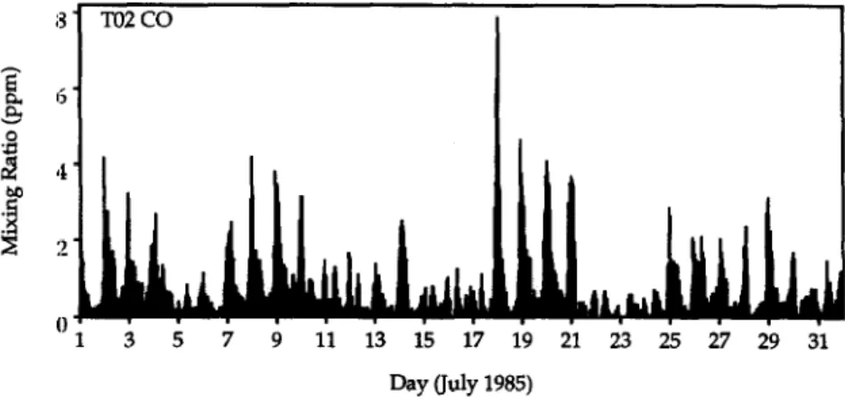
The air quality during the month of July 1985 was quite poor in general, due to the stagnant air conditions caused by the presence of a high-pressure system to the southwest of the Lower Fraser Valley (Hedley and Singleton, 1997). Evidence of the stagnation of the lower troposphere during 17-21 July is clearly shown in the month long time series of CO measurements taken at the urban station TO2 for July 1985 (Fig. 2; see Fig. 1 for the station locations). Carbon monoxide is relatively unreactive, and local concentrations are mainly affected by local emissions, advection and dif- fusion. On many days during the month, very large spikes in CO mixing ratio are observed, with peak values occurring near midnight. The cause of these

peaks is most likely due to the formation of nighttime surface inversions, where even weak emissions of CO can lead to large ambient concentrations. On midnight of 17 July, the observed value of CO was almost 8 ppm.

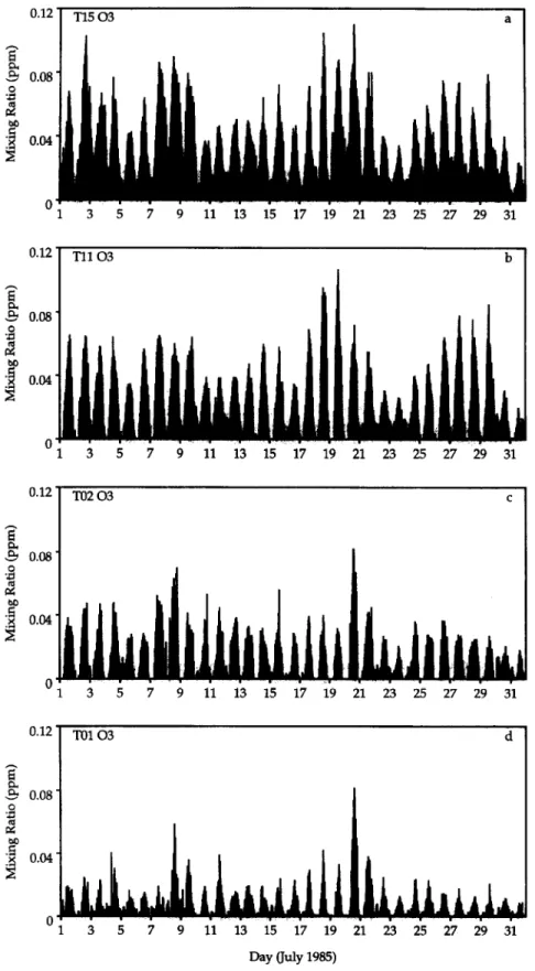
The time series of hourly ozone mixing ratio for the entire month at station T15 is shown in Fig. 3a. On six days (2,7,8,18-20 July) the ozone mixing ratio exceeded the 1 h Canadian air quality objective of 82 ppb, and on three of those days, the ozone mixing ratio exceeded 100 ppb. The peak mixing ratio measured within the Lower Fraser Valley for the whole month of July was 110 ppb, and was measured at T15 on 20 July.

Station Tll is farther into the rural portion of the Lower Fraser Valley than T15, but the time series of ozone has the same qualitative features (Fig. 3b). The ozone levels at Tll tend to be less than those at T15, especially at night. The high ozone days appear to cluster together into multi-day episodes which are similar between the two time series plots. The ozone exceedances observed during the first ten days of the month at T15 are not apparent at Tll. The two episodes occurring in the last half of the month from 17-21 July to 26-29 July are clearly visible in both time series.

The ozone measurements taken at an urban site TO2 are shown in Fig. 3c. Compared to the sites outside of the urban core, the ozone levels are very much lower at T02. This is expected, since the urban core is characterized by high concentrations of freshly emitted NO, which reacts quickly with any ambient ozone. At this station, there is only one day that experiences an exceedance, when on 20 July the mixing ratio just barely reached 82 ppb. It is notable that this happened to be a Saturday, when one would expect that anthropogenic emissions of ozone precursors are significantly lower than on a weekday.

At the Robson Square station (TOl), the ozone mixing ratios are lower yet (Fig. 3d), with the one exception of 20 July, where the same ozone spike is seen as at T02. It appears that this urban ozone spike is a robust feature in the observations. The rural sites

21 23 25 27 29 31

Day (July 1985)

(5)

1620 M. HEDLEY et al. T15 03 a

3 B

0.08

.2

d

I

0.04 n. . . . . . . , . “1 3 5 7 9 11 13 15 17 19 21 23 25 27 29 31 b “ 1 3 5 7 9 11 13 15 17 19 21 23 25 27 29 31 0.12 _{T o1 03} _d 9 11 13 15 17 19 21 23 25 27 29 31

Fig. 3. Time series of ozone mixing ratios for July 1985 at station (a) T15, (b) Tll, (c) T02, and (d) TOl. do not exhibit this particular phenomenon, and in fact It is interesting that during the observed ozone the rural sites show that the episode is rapidly episodes, the night time surges of CO that were noted decaying on 20 July. This feature will be commented at T O2 are even more significant than usual. This is on in more depth in a later section. evidence that the conditions for the development of an

(6)

ozone episode are closely related to the state of the lower atmosphere.

The rest of the paper will focus on the 17-21 July ozone episode.

3. MODEL EVALUATION

The horizontal domain for CALGRID is the same as that shown in Fig. 1. It is a 240 km x 240 km square on a Universal Transverse Mercator (UTM) projec- tion. The horizontarl resolution used for this domain is 5 km, which was chosen to match the resolution of the emissions database. The depth of the photochemical grid is set to 5 km and is divided into 10 levels of varying depth (Table 1).

Table 1. Heights of the layer faces for the photochemical simulation

Level _zf@) Level

zyxwvutsrqponmlkjihgfedcbaZYXWVUTSRQPONMLKJIHGFEDCBA

Zf b-4

11 5000 5 260 10 3600 4 160 9 2200 3 80 8 1200 2 20 I 660 1 0 6 4LO

The meteorological simulation was carried out using MC2 on a larger domain, and then processed using CALMET to produce the meteorological data set that CALGRID requires on the above grid. A full description of the performance of the MCZCALMET model combination was given by Hedley and Single- ton (1997).

For the photochemical simulation, the initial mixing ratios of the trace pollutants were set to values typical for a clean rural atmosphere as follows: O3 = 15 ppb (parts per billion), NO, = 2 ppb,

NMOC = 17 ppbC (ppb of carbon) and

CO = 200 ppb. The decision to begin with such clean initial conditions was based on the belief that the emissions themselves would eventually drive the simulation towards realistic pollutant concentrations.

The processing of the episode-specific emissions data used in the following simulations were described in detail by McLaren et al. (1996). The anthropogenic emissions of NO for 0800 PST on 17 July are shown in Fig. 4. The large rush hour emissions clearly show the location of the urban core of Vancouver.

The simulation was initiated at 0400 PST, 17 July and run for 116 h until 0000 PST 22 July. All calculations were performed on a Silicon Graphics Power Indigo2 desk top workstation with 64 Mbytes of

memory. The CPU requirements for the MC2

zyxwvutsrqponmlkjihgfedcbaZYXWVUTSRQPONMLKJIHGFEDCBA

5550

450

500

550

600

io i0 3b 40

Fig. 4. Anthropogenic NO emissions for 0800 PST on 17 July. The shading indicates the magnitude of the emissions in terms of g s- 1 per grid cell according to the gray scale shown.

(7)

1622 M. HEDLEY et al. simulation were 40 min of CPU time for every hour of

simulated time. The CALGRID simulation required 1.5 h of CPU time for every 24 h of simulation.

3.1.

zyxwvutsrqponmlkjihgfedcbaZYXWVUTSRQPONMLKJIHGFEDCBA

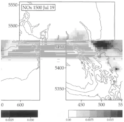
Surface fields

The simulated surface mixing ratio field for NO, on 19 July at 1500 PST is shown in Fig. 5. The peak values occur over the urban core of the city of Van- couver. A plume of NO, extends downwind from the urban core, extending along the Lower Fraser Valley. Note the locations of the secondary maxima along the Washington coastline and on Vancouver Island, which are caused by large industrial point source emissions.

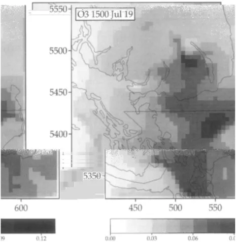
The surface CO mixing ratio for 19 July at 1500 PST (Fig. 6) shows how the urban plume extends into the Lower Fraser Valley more clearly than NO,, due to its longer chemical lifetime. The ozone field for this time (Fig. 7) reveals that the model predicted over 100 ppb in some areas. The peak value of 106 ppb occurred on the American side of the border south of Chilliwack. Just to the west of Harrison Lake, there were also a few grid points with greater than 100 ppb. Another local maximum is located near Abbotsford, with values greater than 80ppb. Directly over the urban core of Vancouver, it is seen that there is a local

minimum of ozone. This is due to the titration of ozone by the local sources of NO emitted from auto- mobiles, via the reaction

NO+O,+NO,+O,. 3.2. Statistical evaluation

A quantitative assessment of the accuracy of the base case model prediction can be made using the statistical measures suggested by Willmott (1981, 1982) and Willmott et al. (1985), as Steyn and McKendry (1988) did in evaluating their meteorological simulation of the Lower Fraser Valley. We use the same terminology and definitions as presented in those papers and in Hedley and Singleton (1997), including the observed and modelled means and standard deviations of the data; the slope, b, and the intercept, a, of the least-squares linear regression of predicted vs observed data; the root-mean-squared difference, E, between the modelled data (Pi) and observed data (0,); and the index of agreement, d,

calculated as

zyxwvutsrqponmlkjihgfedcbaZYXWVUTSRQPONMLKJIHGFEDCBA

d=l- E=

<(ICI + lW >

where the primed quantities are the departures from the mean observed value, and the angle brackets

‘\\

zyxwvutsrqponmlkjihgfedcbaZYXWVUTSRQPONMLKJIHGFEDCBA

W x 1500 Jd 191

450

500

550

600

0.00

zyxwvutsrqponmlkjihgfedcbaZYXWVUTSRQPONMLKJIHGFEDCBA

0.0075 0.015 0.0225 0.030

Fig. 5. Simulated surface mixing ratio fields at 1500 PST, 19 July for NO,. The gray scales show the mixing ratios in parts per million (ppm).

(8)

Fig. 6. Simulated surface mixing ratio of carbon monoxide at 1500 PST, 19 July. The gray scales show the mixing ratios in parts per million (ppm).

denote the averaging operator. A value of

zyxwvutsrqponmlkjihgfedcbaZYXWVUTSRQPONMLKJIHGFEDCBA

d = 1

indicates perfect agreement, and d = 0 indicates abso- lutely no agreement.

There are many other measures that have been used to evaluate photochemical model performance. In Jiang et al. (1996b) we used a slightly modified version of the measures suggested by Tesche (1988) to compare the performance of MC2-CALGRID against the SAIMM/UAM-V modelling system in simulating the first four days of the ozone episode discussed in this paper.

As recommended by Willmott (1981), E is further decomposed into two parts, Es and EU, which repres- ent the systematic and unsystematic portions of E, respectively. The systematic component is the RMS difference between the observed data and the least- squares linear regression of the predicted vs observed data, P* = a + bOi, while the unsystematic component is the rms difference between the predicted data and PT. The systematic component is caused entirely by non-zero values of the linear regression intercept (a), and values of the slope (b) unequal to one. The unsystematic component is due to any nonlinear variation of the predicted values against observations. The relation E2 = Ef + E& was shown by Willmott (1981). Interpretations of the above parameters are provided by Willmott (1981,1982) and Willmott et a[.

(1985), and summarized by Hedley and Singleton (1997).

In this study, as in Hedley and Singleton (1997), the averages calculated in the above definitions are averages over time, and the statistics are calculated for each observing station. By calculating the performance statistics for each station, systematic errors in the forecast caused by local effects are clearly high- lighted, as will be shown below.

The NO, time series for TO4 (Fig. 8a) reveals that the model accurately predicts daytime NO, levels for the first 3 days of the simulation. The plot of predicted vs observed NO, (Fig. 8b) shows a fairly good linear agreement with a slope of 0.49 and intercept of 14 ppb. It should be noted that only daytime measurements are included in the observed NO, data since the observed extremely high nighttime values proved almost impossible to simulate. Although there were no nighttime measurements of mixed layer depths taken, it is reasonable to assume that the observed high nighttime values of NO, were due to emissions into a shallow nocturnal surface inversion. Hedley and Singleton (1997) showed that the meteorological simulation had difficulty in predicting temperatures and mixed layer depths at overland sites within a small number of grid points of the shoreline, due to an overestimation of the moderating effect of water

(9)

1624 M. HEDLEY et al.

zyxwvutsrqponmlkjihgfedcbaZYXWVUTSRQPONMLKJIHGFEDCBA

5550

5500

5450

5400

5350

500

600

0.03 0.06 0.09 0.12

Fig. 7. Simulated surface mixing ratio fields at 1500 PST, 19 July for ozone. The gray scales show the mixing ratios in parts per million (ppm).

temperatures on air temperatures. Slight errors in the mixing parameters near the surface can lead to large errors in the forecast nighttime boundary layer, and therefore large errors in the forecast concentrations.

The NO, performance results are shown in Table 2 for all the other stations. With the exception of T15 and T16, the indices of agreement for NO, are all above 0.5, with a maximum value of 0.83 at T05. The predicted observed averages are acceptably close for all stations, except possibly for T15 and T16. In general, the model tends to underpredict the standard deviations, although for the urban sites TO2 and TO3 the standard deviations were overestimated. Total RMS errors were less than 20ppb at all sites except T15. It should be noted that no attempt was made to adjust the observed NO, data to correct for possible interference from the presence of nitrates, which can cause overestimation of observed NO, by about 10%. The measured and predicted CO time series for TO4 is shown in Fig. 8c. As with the NO, data, it should be noted that only daytime measurements are included in the observed data. In general, the model performs well at capturing the day-to-day variation in overall CO concentration. The model tends to overestimate CO at rush hours, and it appears that the rush hour

cycle is more pronounced in the model results than in the observed data.

The plot of predicted vs observed CO at TO4 (Fig. 8d) follows a reasonably linear relationship, although the least-squares slope is rather low and the intercept is high (Table 3). The relatively small value for Eu _{is quantitative evidence that the linear relation-}

ship is robust. The index of agreement for this station of 0.67 is encouragingly high.

The performance statistics for the other CO measuring stations are also listed in Table 3. The two stations closest to the urban core, TO8 and T02, have the lowest indices of agreement. The poor performance of the model in the downtown core is likely due to errors in the boundary-layer depth and other surface mixing parameters resulting from the proximity of the urban stations to the coast. The large emissions arising from the urban core into the boundary layer make the model very sensitive to any errors in the boundary-layer calculations. At T03, which is just south of the urban core, the performance is better, and farther inland at TlO the results are still better.

It is clear that the distribution of NO, and CO monitoring sites is too closely grouped around the urban core. This makes hourly measurements too sensitive to local emissions rates and therefore difficult

(10)

TrNox

a 0

X008

4 . a 2 0.06 al g 0.04 0.02 2.5 -17 18 19 20 21 22 - 0 0.02 IX04 0.06 0.08 0.1 0.12 To40 Day (July 1985) C 2.5 3 2.0 8 1.5 % 3 -g 1.0 Z 0.5 Observed (ppm) d -17 18 19 20 21 22 0 0.5 1.0 1.5 2.0 2.5 Day (July 1985) e 19 20 Day (July 1985) 0.12 Observed (ppm) 0 0 0.02 0.04 0.06 0.08 0.1 0.12 Observed (ppm)

Fig. 8. Station TO4 time series and scatter plots of predicted and observed mixing ratios. Time series: (a) NO,, (c) CO, and (e) ozone. Observed values are plotted as circles. Scatter plots of(b) NO,, (d) CO, and (f) ozone. The least-squares linear regressions are indicated by the thick lines. The dashed lines have slopes

of unity and intercepts of zero, representing perfect forecasts.

Table 2. NO, time-series statistic?

Station n (co> cc,> 6, 6, b a E ES EIJ d

TO2 TO3 TO4 TO5 TO7 T10 T14 T15 T16 27 34.6 43.5 7.5 20.0 1.72 - 15.9 18.3 10.3 15.1 0.55 33 19.5 25.4 12.7 13.5 0.62 13.4 13.3 7.6 10.9 0.73 28 47.5 37.3 17.7 14.8 0.49 14.0 17.9 13.5 11.8 0.67 33 55.1 55.4 27.2 17.1 0.49 28.5 17.3 13.7 10.6 0.83 33 24.3 28.4 10.4 9.5 0.42 18.1 11.0 1.2 8.3 0.66 33 32.1 25.0 11.1 8.8 0.34 14.2 12.9 10.1 7.9 0.58 33 32.6 30.9 14.0 10.9 0.47 15.6 11.4 7.5 8.6 0.76 32 27.4 11.5 12.0 5.5 - 0.04 12.5 20.8 20.1 5.3 0.44 23 29.9 19.5 13.7 6.6 0.04 18.3 17.8 16.6 6.4 0.47

“The terms n, b and d are dimensionless. All other terms have dimension ppb. The o and p subscripts refer to observed and predicted values, respectively. The standard deviations are represented by b. The time-averaged species mixing ratios are denoted by (c).

(11)

Table 3. Carbon monoxide time-series statisticsa

Station n (c,) (c,) 6, 6, h a E Es Eu d TO2 55 359 1145 212 568 1.37 652 925 789 483 0.32 TO3 33 1008 629 198 229 0.07 559 471 421 225 0.40 TO4 54 167 849 361 247 0.35 584 326 248 211 0.67 TO8 55 524 1003 312 955 1.29 327 987 488 858 0.37 TlO 33 488 660 225 203 0.26 532 305 237 191 0.46 “The terms n, b and d are dimensionless. All other terms have dimension ppb. The o and p subscripts refer to observed and predicted values, respectively. The standard deviations are represented by 6. The time-averaged species mixing ratios are denoted by (c).

Table 4. Ozone time series statisticsa Station TO1 109 14.3 11.6 18.3 8.8 0.34 6.8 13.9 12.4 6.3 0.70 TO2 114 17.4 14.2 19.8 11.4 0.47 6.1 12.8 10.9 6.6 0.82 TO3 67 14.5 17.6 16.0 14.7 0.85 5.2 6.6 3.8 5.4 0.95 TO4 92 24.8 20.9 20.3 11.0 0.44 9.9 13.5 11.9 6.3 0.80 TO5 115 27.5 17.9 23.4 10.6 0.35 8.1 19.0 17.9 6.6 0.70 TO6 59 19.2 17.8 17.7 10.4 0.42 9.8 12.6 10.4 7.2 0.78 TO7 116 38.4 26.4 25.1 13.2 0.39 11.3 21.3 19.4 8.7 0.70 TO9 116 32.6 27.0 30.5 13.0 0.30 17.1 23.7 21.9 9.1 0.68 TlO 48 33.7 30.0 24.5 12.7 0.25 21.5 21.5 18.4 11.0 0.60 Tll 116 32.0 45.3 29.8 16.7 0.43 31.5 24.1 21.5 10.8 0.76 T12 114 35.5 46.9 32.0 13.4 0.30 36.1 26.6 24.9 9.2 0.69 T13 55 28.1 23.0 12.8 12.0 0.66 4.6 10.9 6.7 8.6 0.79 T15 115 44.5 34.3 27.7 16.8 0.43 15.2 22.2 18.8 11.8 0.74 T16 93 31.3 31.0 30.1 16.3 0.40 18.5 20.9 17.9 10.8 0.78 “The terms n, b and d are dimensionless. All other terms have dimension ppb. The o and p subscripts refer to observed and predicted values, respectively. The standard deviations are represented by S. The time-averaged species mixing ratios are denoted by (c>.

to compare against model predictions. It would be highly beneficial to have more monitoring sites located farther inland and away from major highways and industrial facilities.

The ozone time series for TO4 (Fig. Se) shows that with the exception of the second to last day, the model predicts ozone mixing ratios well. (Note that for the ozone time series, nighttime observations are included in the graphs and the subsequent analysis.) The peak values are underestimated by about 10 ppb each day except Saturday, 20 July, when the peak mixing ratio was underestimated by over 33 ppb. The model predicted nighttime increases in ozone that were somewhat high, although the results for the early morning of 20 July are very good.

The predicted ozone at TO4 shows a good linear relationship with the observed values, although the model shows a tendency to underforecast the peaks and overforecast the minimum values (Fig. 8f). The points are tightly grouped about the P* line, with an unsystematic RMS error component of only 6 ppb (Table 4). The modelled average mixing ratio was off by -4 ppb, and the predicted standard deviation was about half of the observed 20 ppb. The overall performance of the simulation at this station was very acceptable with an index of agreement of 0.81.

The occurrence of a large ozone surge on a Satur- day is curious, and was measured at several sites in the downtown and surrounding area (see Fig. 3d for the TO1 time series). It was not reported in the rural areas, such as Tll (Fig. 3d). It is possible that it was caused by left over precursors and ozone from the Friday which were subsequently mixed down to the surface on Saturday afternoon, an event not captured by the model. The absence of any significant morning rush hour on Saturday would lead to reduced destruction of ozone, and thus higher observed ozone concentrations. The failure of the model to predict this effect may be an indication the modelled nighttime drainage flow was too efficient at cleaning the Lower Fraser Valley of ozone and its precursors on the Friday night.

The performance statistics for ozone predictions at all stations are listed in Table 4. The model performs extremely well for most stations, with indices of agreement ranging from 0.60 to 0.95. The high precision of the model is indicated by the small values of EU, which are less than or equal to 12 ppb for all stations; in other words, the model results vary almost linearly with the observations.

The relatively large values of the linear regression intercept, a, for the rural stations Tll and T12 indicate

(12)

0.12 0.12

X OS1 0.1

.*

(13)

-0.8 0.0 0.8 1.6 2.4

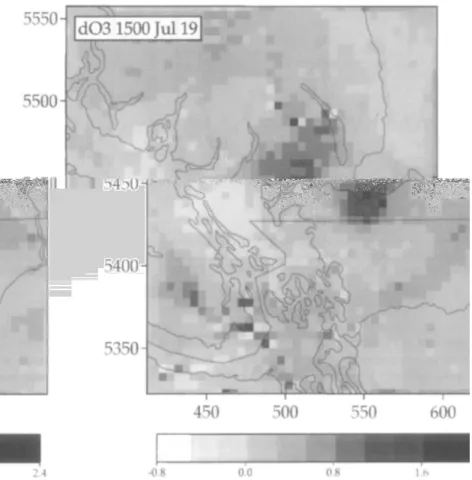
Fig. 10. Surface ozone differences between the experiments run using the default SCAQS-based and the Lower Fraser Valley-based mechanistic parameters for 1500 PST, 19 July. The gray scale shows the

differences in mixing ratios in ppb.

zyxwvutsrqponmlkjihgfedcbaZYXWVUTSRQPONMLKJIHGFEDCBA

4. SUM M ARY AND DISCUSSION

The results of the detailed quantitative error analysis show that the MCZCALGRID photochemical modelling system predicts the photochemical situation with acceptable precision for the five day simulation presented.

Daytime values of the nitrogen oxide and carbon monoxide concentrations were predicted reasonably well at most sites, including the urban core. The model tended to underpredict peak ozone, but in general there was a highly linear relationship between predicted and observed ozone. The model failed to capture the surge of ozone that occurred on the Satur- day in the urban core, and the nighttime concentrations at the rural sites was overestimated.

The mechanistic parameters are very sensitive to the organic emissions profile, and a brief comparison of the parameters resulting from the SCAQS emissions profile and the Lower Fraser Valley profile illustrated the large differences that result from relatively small profile changes.

The net impact of these differences on ozone production was shown to be relatively minor in this case, but larger effects could occur in control strategy simu-

lations. Future work will include examination of other groupings of lumped NMOCs that are less sensitive to reasonable changes in emissions profiles.

One of the most significant problems in validating a modelling system in the Lower Fraser Valley is that the distribution of monitoring stations is too dense in the urban core and too sparse everywhere else. It would be highly beneficial to have several stations located farther up the valley, and to have at least one station in the northern part of the Strait of Georgia to measure the pollutant concentrations of the air par- cels that eventually enter the valley.

An area that we have not examined in this study is the sensitivity of the model results to the details of the dry deposition mechanism and parameters. The ADOM (Venkatram et al., 1988) style of dry deposition for ozone is employed in CALGRID, and recent

work by Padro

zyxwvutsrqponmlkjihgfedcbaZYXWVUTSRQPONMLKJIHGFEDCBA

et al. (1992) has identified canopy

wetness, among other factors, as having an important influence on deposition velocities.

Recent studies have suggested that deficiencies in model predictions of ozone are due primarily to un- certainties in the NMOC emissions estimates, parti- cularly from motor vehicles and vegetation. For example, Harley et nl. (1993) simulated the 27-29

(14)

August 1987 SCAQS intensive monitoring period. using the CIT photochemical model, and underpre- dieted ozone levels by about 23% on average. They then used the results of a tunnel study in Los Angeles to justify an increase of organic gas emissions from en- gine exhaust by a factor of 3, which significantly improved the ozone forecast. Recent work by Geron er al. (1994) shows that the biogenic emissions produced by BEIS can be a factor of 5 -10 too low when compared against measurements for certain U.S. counties and certain types of vegetation.

Although these studies present evidence that the NMOC emissions can be problematic, there is no comparable evidence that the mobile or biogenic emissions inventories are underestimated in the present study. The recient Cassiar Tunnel study in Van- couver indicated that the mobile emissions model MOBILESC, the Canadian version of MOBILESa that was used to develop the mobile emissions for the Canadian portion of the domain, adequately represented light duty vehicle emission factors for the driv- ing conditions in the tunnel (Gertler et al., 1996).

Unfortunately, there has not yet been an evaluation of the biogenic emissions model for the land cover type in the Lower Fraser Valley. Our own sensitivity studies with the MC2,CALGRID system show that increased NMOC emissions, especially in the urban regions, would improve the model performance for ozone. However, in the current study, there are no NMOC measurements to compare against (although the NMOC concentrations produced by the model are within the range of variability of observations for later years reported by Dann, 1994) and therefore we have no basis on which to modify the anthropogenic or biogenic emissions estimates.

Although it is clear there is room for improvement, the above results are encouraging. The model adequately captured the general features of the ozone episode without arbitrary adjustments to the emissions inventory. The next stage of this study will be to evaluate a number of emissions control strategies using this simulatl.on as the base case scenario. In addition, the sensitivity of the model to changes in emissions, meteorological grid spacing, deposition parameters and chemical mechanism details will be presented in future papers. Finally, in order to estab- lish further the accuracy of the MCZ-CALGRID modelling system, the Pacific 93 episode (Steyn et al.,

1996) will be simulated and compared against the rich set of measurements made during that intensive monitoring operation.

Acknow ledgements- The authors thank MS S. Bohme and Mr A. Dorkalam for their work on preparing the emissions data sets for this study. The quality control procedures for the emissions inventory processing implemented by MS Bohme are especially appreciated. This research was funded by Natural Resources Canada through the Panel on Energy Research and Development and by the National Research Council of Canada.

REFERENCES

Canadian Council of Ministers of the Environment (1990) Management PIun for Nitrogen O xides (NO ,) and

Volatile O rganic Compounds (VO Cs) Phase I. ISBN O- 191074-70-7.

Carter, W. (1990) A detailed mechanism for the gas-phase atmospheric reactions of organic compounds. Atmo- spherii Environment 24A, 481- 318. _

Dann. T.. Wane. D.. Steenkamer. A.. Halman R. and Lister. M. (1994)‘Volazle organic compound measurements in’the Greater Vancouver Regional District (GVRD) 1989-1992. Report No. PMD 94-1, Technology Development Direc- torate, Environmental Technology Centre, Environment Canada.

Gardner, L., Causley, M., Wilson, G. and Jimenez, M. (1992) User’s Guide for the Urban Airshed M odel Volume IV: User’s M anual for the Emissions Preprocessor Sy stem 2.0,

SYSAPP-92/059a, Systems Applications International, San Rafael, California.

Geron, C. D., Guenther, A. B. and Pierce, T. E. (1994) An improved model for estimating emissions of volatile organic compounds from forests in the eastern United States. J. aeoDhvs. Res. 99. 12.773-12.791.

Gertler, A. W., Wittorff, D. N., McLaren, R., Belzer, W. and Dann, T. (1996) Characterization of vehicle emissions in Vancouver BC during the 1993 Lower Fraser Valley Oxidants study. Atmospheric Environmenf (in press). Harley, R. A., Russell, A. G., McRae, G. J., Cass, G. R. and

Seinfeld, J. H. (1993) Photochemical modeling of the Southern California air quality study. Enuir. Sci. Technol. 27, 378- 388.

Hedley, M. A. and Singleton, D. L. (1997) Evaluation of an air quality simulation of the Lower Fraser Valley-Part I. Meteorology. Atmospheric Environment 31, 1605- 1615.

Jiang, W., Singleton, D. L., McLaren, R. and Hedley, M. (1996a) Sensitivity of ozone concentrations to rate con- stants in a modified SAPRC90 chemical mechanism used for Canadian Lower Fraser Valley ozone studies. Atmo- spheric Environment (in press).

Jiang, W., Hedley, M. and Singleton, D. L. (1996b) Compari- son of the MCZ/CALGRID and SAIMM/UAM-V photochemical modelling systems in the Lower Fraser Valley, British Columbia. Atmospheric Environment (submitted).

Kumar, N., Russell, A. G., Tesche, T. W. and McNally, D. E. (1994) Evaluation of CALGRID using two different ozone episodes and comparison to UAM results. Atmospheric Environment 28, 2823- 2845.

Lawson, D. R. (1990) The Southern California air quality study. 1. Air W aste M an. Ass. 40, 156- 165.

McLaren, R., Bohme, S., Hedley, M., Jiang, W., Dorkalam, A. and Singleton, D. L. (1996)Emissions-inventory processing for UAM-V and CALGRID modelling in the Lower Fraser Valley. The Emission Inventory: Programs and Pro- gress, VIP- 56, 749- 755, Air and Waste Management Association. Pittsburgh, Pennsylvania.

National Research Council (1991) Rethinking the O zone Problem in Urban and Regional Air Pollution. National Academy Press, Washington, DC.

Padro, J., Neumann, H. H. and Den Hartog, G. (1992) Modelled and observed dry deposition velocity of 0s above a deciduous forest in the winter. Atmospheric Environment 26, 175- 784.

Pierce, T. E. and Waldruff, P. S. (1991) PC-BEIS: a personal computer version of the Biogenic Emissions Inventory System. J. Air W aste Man. Ass. 41, 937-941.

Pilinis, C., Kassomenos, P. and Kallos, G. (1993) Modeling of photochemical pollution in Athens, Greece-application of the Rams-Calgrid modeling system. Atmospheric Environment 27B, 353- 370.

Steyn, D. G. and McKendry, I. G. (1988) Quantitative and qualitative evaluation of a three-dimensional mesoscale

(15)

1630 M. HEDLEY et a/. numerical model simulation of a sea breeze in complex

terrain. Mon. We&. Reo. 116, 1914-1926.

Steyn, D. G., Bottenheim, J. W. and Thomson, R. B. (1996) Overview of tropospheric ozone in the Lower Fraser Valley, and the PACIFIC ‘93 field study. Atmospheric

Enoirknent (submitted).

Tanguay, M., Robert, A. and Laprise, R. (1990) A semi- implicit semi-Lagrangian fully compressible regional forecast model. Mon. We&. Rev. 118, 1970-1980.

Tanguay, M., Yakimiw, E., Ritchie, H. and Robert, A. (1992) Advantages of spatial averaging in semi-implicit semi-Lagrangian schemes. Mon. Weath. Rev. 120, 113-123.

Tesche, T. W. (1988) Accuracy of ozone air quality models.

J. Envir. Engng 114, 739-752.

Venkatram, A., Karamchandani, P. K. and Misra, P. K. (1988) Testing a comprehensive acid deposition model.

Atmospheric Environment 22, 737- 747.

Willmott, C. J. (1981) On the validation of models. Phy s. Geography 2, 168- 194.

Willmott, C. J. (1982) Some comments on the evaluation of model performance. Bull. Am. M et. Sot. 63, 1309-1313. Willmott, C. J., Ackleston, S. G., Davis, R. E., Feddema, J. J.,

Klink, K. M., Legates, D. R., O’Donnell, J. and Rowe, C. M. (1985) Statistics- for the evaluation and comparison of models. J. geoohvs. Res. 90. 8995-9005.

Yamartino, R.-J., s&e, J. S., Carmichael, G. R. and Chang Y. S. (1992) The CALGRID mesoscale photochemical grid model-I. Model formulation. Atmospheric Environment 26A, 1493- 1512.