Publisher’s version / Version de l'éditeur:
Vous avez des questions? Nous pouvons vous aider. Pour communiquer directement avec un auteur, consultez la première page de la revue dans laquelle son article a été publié afin de trouver ses coordonnées. Si vous n’arrivez pas à les repérer, communiquez avec nous à PublicationsArchive-ArchivesPublications@nrc-cnrc.gc.ca.
Questions? Contact the NRC Publications Archive team at
PublicationsArchive-ArchivesPublications@nrc-cnrc.gc.ca. If you wish to email the authors directly, please see the first page of the publication for their contact information.
https://publications-cnrc.canada.ca/fra/droits
L’accès à ce site Web et l’utilisation de son contenu sont assujettis aux conditions présentées dans le site LISEZ CES CONDITIONS ATTENTIVEMENT AVANT D’UTILISER CE SITE WEB.
Internal Report (National Research Council of Canada. Institute for Research in Construction), 1996-01-01
READ THESE TERMS AND CONDITIONS CAREFULLY BEFORE USING THIS WEBSITE. https://nrc-publications.canada.ca/eng/copyright
NRC Publications Archive Record / Notice des Archives des publications du CNRC : https://nrc-publications.canada.ca/eng/view/object/?id=3188d842-4c89-48a3-b929-52208a5fc207 https://publications-cnrc.canada.ca/fra/voir/objet/?id=3188d842-4c89-48a3-b929-52208a5fc207
Archives des publications du CNRC
For the publisher’s version, please access the DOI link below./ Pour consulter la version de l’éditeur, utilisez le lien DOI ci-dessous.
https://doi.org/10.4224/20359107
Access and use of this website and the material on it are subject to the Terms and Conditions set forth at An International Comparison of Room Acoustics Measurement Systems
I
I
An International Comparison
of
Room Acoustics Measurement
Systems
by J.S. Bradley
IRC Internal Report IRC-IR-714
January 1996
SUMMARY
This report presents the results of comparisons of 23 different room acoustics measurement systems. The round robin comparisons were obtained by shipping a
digital reverberator to each measurement group. Three preset settings of the reverberator were used to represent three different standard rooms that each group measured. Comparisons were made for octave band values of eight different room acoustics quantities as well as RASTI values. The eight quantities were:
c50,
early-to-late arriving sound energy ratio with 50 ms early time limit;cso,
early-to-late arriving sound energy ratio with 80 ins early time limit;TS : centre time;
EDT, early decay time;
RT,
reverberation time;IACC(e) inter-aural cross correlation of the early sound; IACCO), inter-aural cross correlation of the late sound; IACC(t), inter-aural cross correlation of the total sound.
Using one measurement system, nine measurements of the reverberator over the one-year period of the round robin tests were used to assess the reproducibility of the measurements. These showed that the measurement results were very
accurately reproducible and that the round robin test procedure was a valid comparison of the various measurement systems.
Averages of the better clustering results from the various measurement systems were determined to estimate the correct values of each measurement. The standard deviation of these better clustering results were used to assess the accuracy of each measurement system and a simple rank ordering of the measurement systems was calculated. Approximately 213 of the measurement systems produced results of at least reasonable accuracy.
Two specific problems were identified. Different calculation procedures produced quite different EDT values for decays with strong direct sound components. Impulse responses with prominent strong reflections close to the early time interval limit led to more variable low frequency Cso values.
Recommendations are given for improved procedures to minimize these two specific problems. It is also strongly recommended that in the future all room acoustics measurement systems be validated to verify the accuracy of the calculated room acoustic quantities.
CONTENTS
1
.
Introduction...
3...
2.
Procedures and Participants 5 2.1 Test Procedure...
52.2 Analysis Procedures
...
82.3 Participants
...
10...
3.
Reproducibility of the Measurements 13...
4.
Measures from Integrated Impulse Responses 19 4.1 Comparisons of Results...
19. .
...
4.2 Specific Problems 90...
4.3 Comparisons with Reproducibility 91...
4.4 Ranking of the Measurement Systems 93 5.
Comparisons of Inter-Aural Cross Correlations...
95...
6.
Comparisons of RASTI Measurements 121 7.
Discussion and Conclusions...
1257.1 Reproducibility
...
1257.2 Comparisons with Subjective Difference Limen ... 125
7.3 The State of the
Art
...
127...
7.4 Recommendations 128 Acknowledgments...
1291.
INTRODUCTIONThis report provides comparisons of the results of 23 different room acoustics measurement systems. These round robin comparisons were obtained by using a digital revbaberator to represent standard rooms, and by sending the digital
reverberatx to each measurement group. (An ALEX digital reverberator donated by Lexicon was used.) Although the participants are listed in this report, the results are presented anonymously. It was not the intent of this study to embarrass participan~s, but to provide them with a guide for possible improvements to their measurement systems. However, the results of our own measurement systems, RAMSoft-I1 and RAMSoft-3, are identified. It is hoped that the result of these comparisons will be a significant improvement in the accuracy of room acoustics measurements throughout the world.
This work was stimulated by earlier comparative measurement studies supported by the Concert Hall Research Group and the development of a new version of the I S 0 3382 standard "Measurement of the reverberation time of rooms with
reference to other acoustical parameters". In the summer of 1992, three research groups made comparative measurements in nine auditoria in the North Eastern U.S.A. These groups and their leaders were: the National Research Council of Canada (John Bradley), the Danish Technical University (Anders Gade), and the University of Florida (Gary Siebein). The results of these comparisons were reported in a number of papers[l-61 and have led to further changes and improvements to the measurement systems used by these three groups.
The present round robin comparisons are an attempt to look at one of the parts of the overall problem of room acoustics measurement system accuracy. These round robin comparisons have focused only on the problems related to the measurement system algorithms and have not considered other effects related to the use of different transducers and their placement. Studies of these other aspects have been reported[7-91 and indicate there are significant sources of error related to the use of different transducers and the placement of the transducers. By concentrating first on the basic measurement system algorithms, it is hoped to resolve problems in this area before going on to consider the potentially larger effects of transducer types and their positioning during measurements in actual rooms.
The new draft of I S 0 3382 includes definitions of a number of newer types of auditorium acoustics measures. The suggested importance of these quantities and the standardized definitions included in IS0 3382 are intended to encourage more measurements of these quantities. As a part of this progress to a more quantitative approach to room acoustics problems, it is of course necessary to understand and attempt to minimize measurement errors and uncertainties. It is hoped that these round robin results will contribute to this process.
2. PROCEDURES AND PARTICIPANTS
2.1 Test Procedure
Each measurement group was asked to measure three different settings of the ALEX reverberator which would be equivalent to measuring three different rooms. Participants were provided with abbreviated instructions to tell them exactly how to use the reverberator. It is possible to adjust many details of the reverberator settings so that several thousand combinations are possible. To avoid errors, only three preset configurations were used. Thus, each user only had to turn a single knob and select preset memory 3, 10, or 11. The ''wetldry" control on the reverberator was fixed so that the relative amplitude of the direct pulse did not vary. Users also adjusted the input and output level controls.
Figures 1,2, and 3 show the initial parts of the impulse responses of the three reverberator settings used in the comparisons. They look a little different than typical room impulse responses, but were chosen from the available preset settings to provide a reasonable range of conditions and to provide values of the various acoustical parameters that were similar to those expected in real rooms. The results of the comparisons indicate that the choice of reverberator settings was successful in that each setting challenged the measurements systems in different ways. Preset 03
I
--
8 0 0.05 0.1 0.15 0.2 0.25 0.3 0.35 Time, sPreset 10
0 0.05 0.1 0.15 0.2 0.25 0.3 0.35
Time, s
Figure 2. Initial part of the impulse response of ALEX reverberator preset 10.
Preset 11
0 0.05 0.1 0.15 0.2 0.25 0.3 0.35
Time, s
Participants were given response sheets that suggested the basic quantities that should be measured and that results were desired in the octaves from 125 to
4000 Hz. They were encouraged to measure other quantities, other variations of
the principal quantities, or in higher or lower octave bands. These extra data have not been included in the present analyses because there were very few comparable results. The present comparisons were made for nine different quantities. Most measurement systems could not measure all nine quantities. Some systems produced as few as one of the nine quantities.
The nine quantities and their definitions are listed below. They correspond as closely as possible to the definitions in IS0 3382.
Two different early-to-late-arriving sound energy ratios were included: CSo and Cso having 50 and 80 ms early time intervals, respectively. They are defined as follows,
where p(t) is the instantaneous pressure response to an impulsive source. For C50, te = 50 ms and for Cso, te = 80 ms.
The Centre Time, TS, which is the centre of gravity of the impulse response, is defined as follows,
The early decay time, EDT, is usually measured from a least squares best fit straight line to the first 10 dB of the reverse integrated Schroeder decay curve considered in terms of decibels versus time.
The reverberation time, RT, is also measured from a least squares best fit straight line to the rzverse integrated Schroeder decay curve considered in terms of decibels versus time. Participants were asked to use the portion of the decay curve between -5 dB and -30 dB relative to the maximum. This was
recornmenrled because experience in real rooms has shown that measurements can almost always be made over this range without the unwanted effects of
background noise. A number of participants provided results for other portions of the decay curve.
Because the ALEX reverberator is a stereo device, participants were also
encouraged to measure Inter-Aural Cross Correlations (IACC). It was suggested that these be measured for the early, late, and total time intervals of the impulse responses. The cross correlation function is calculated as follows,
The Inter-Aural Cross Correlation is calculated as the maximum of the absolute value of the cross correlation function for time s h i i between f 1 ms. Three different variations of the IACC were calculated: IACC(e), IACC(l), and IACC(t) that were obtained using the early, late, and total time intervals of the impulse responses. Again, the early sound is considered to be the first 0.08 s of the impulse response. Thus, the three IACC values can be defined from the above equation and the integration limits in the following table.
Although there are a number of different measures of speech intelligibility,
RASTI has become widelv accented because it is standardized (IEC 286). RASTI IACC(e)
IACC(1) IACC(t)
, L
was developed as a simplification of the Speech Transmission Index, STI. RASTI and ST1 measure the effects of room acoustics by the reduction of the amplitude modulation of signals propagating in a room. They include the influence of the speech-signal-to-ambient-noise ratio on speech intelligibility. Both RASTI and ST1 can be calculated directly from the degradation of the amplitude modulation of steady state test signals or from the Fourier Transform of the squared impulse response. For more complete definitions of the RASTI measure, see references [10,11]. Integration Limits 2.2 Analysis hocedures Ti, s 0 0.08 0
The reverberator was measured nine different times with our own RAMSoft-I1 measurements system over the one-year duration of the round robin
measurements. This was to establish an estimate of the reproducibility of the measurements including the stability of the ALEX reverberator. These
measurements were also to verify that the ALEX reverberator had not changed or become defective over the one-year period. Damage to the unit seemed a
possibility because of the many times that it was shipped from group to group on three different continents. Fortunately, there was never any indication of any damage to the unit. Although the reproducibility results are based on only one measurement system, they can be used to suggest the limit to the possible agreement among the results of the various groups. Differences smaller than the reproducibility differences may not represent real differences between the results of the various measurement systems.
Tz, s 0.08 1 .O 1 .O
It is also possible to compare the differences among measurement results with
.,
subjectivk difference limen for each quantity. Vorlshder[l2] rounded off the subjective difference limen for mid-frequency values of the various quantities established by Cox et.al.[l3]. These approximate subjective difference limen areincluded in Table 1 below.
Table I . Approximate subjective difference limen for mid-frequency values of each quantity. Quantity cso,
dB
cso,dB
TS, s EDT, s RT, s IACC RASTIAn approximate subjective limen for IACC values is also included in Table 1. This was obtained from the work of Cox et al.[13] and is said to be for values of long-time inter-aural cross correlations. These are not the same as the IACC measurements in this round robin but this subjective difference limen may be approximately the same.
Subjective Difference Limen 0.5 dB 0.5 dB 0.01 s 5 % 5 % 0.075 0.015
No published difference limen for RASTI values were found. An estimated subjective difference limen was determined from the published relationship between RASTI (STI) and CsO values Figure 7, reference 141. For an intermediate RASTI (STI) value of 0.5 the 0.5 dB difference limen for Cso in Table 1 would correspond to a 0.015 subjective difference limen for RASTI values. This estimated subjective difference for RASTI values is also included in Table 1.
There are other sources of error associated with complete measurements in rooms, such as those due to the use of different types of transducers and the positioning of these transducers. Thus, it is not adequate for the errors in the present round robin results to be less than these subjective difference limen. It would be desirable that the errors associated with the basic measurement algorithms be much smaller than these subjective difference limen so that they do not contribute significantly to the total measurement errors of real measurements.
It is also necessary to determine some estimate of the correct answer for each of the room acoustics measures of each reverberator setting. This was achieved by calculating the average of the data that best clustered closely together. This excluded results that clearly did not correspond with the common trends of the best clustering data. To minimize errors in estimating these "best" averages, only data from groups that clustered together well for all measures were included. By
this process, approximately half of the data available for each measure was used in determining the "best" average results. The standard deviations of the better results about these "best" averages were also calculated. It is suggested that the results of the better measurement systems should normally fall within two standard deviations of the "best" average values where these standard deviations reflect the variation among the better clustering results.
2.3 Participants
A total of 23 different measurement systems were included in the round robin comparisons. In some cases, one measurement group had more than one measurement system. Some participants used their own custom developed measurement systems while others used commercial systems. In other cases, commercial systems were tested by the manufacturer. In a few cases the
measurement systems were more specialized and only measured a single quantity. Finally, results for some commercial systems were provided by more than one test group. Usually these were different versions of these systems. Table 2 lists the participants including the contact person, the name of the measurement group, and the measurement system.
Measurement
Contact Person Measurement Group System Source Signal
J. Bradley National Research Council, RAMSoft-I1 MLS
Canada
I. Bradley National Research Council, RAMSoft-3 MLS
Canada
M. Barron University of Bath, Custom Pulse and filtered
United Kingdom noise
A. Gade Danish Technical University, Custom Octave sweeps
Denmark
T. Hidaka Takenaka Research Lab., Japan Custom Stretched pulse
H. Tachibana University of Tokyo, Japan Custom Sweep
H. Tachibana University of Tokyo, Japan Custom MLS
G. Marshall Klepper Mashall King Assoc., TEF Chirp Sweep
USA
G. Marshall Klepper Marshall King Assoc., TEF MLS MLS
USA
R. Essert ARTEC, USA Custom 1 MLS
R. Essert ARTFC, USA Custom 2 Multi-part sweep
M. Vorliinder P.T.B., Germany Custom MLS
N. Xiang Head Acoustics, Germany Custom MLS
E. Mommertz Aachen University, Germany Custom MLS
R. Talaske The Talaske Group, USA Custom MLS
W. Chu National Research Council, MLSSA 9 MLS
Canada
G. Soulodre Comaunications Res. Council, MLSSA 8 MLS
Canada
J. O'Keefe Aercwstics Engineering, MLSSA 8 MLS
Canada
J. O'Keefe Aercoustics Engineering, MIDAS Pulse
Canada
K. Hansen Briiel and Kjaer, Denmark B&K 2133 Pink noise
K. Hansen Briiel and Kjaer, Denmark B&K 2231
+
PulseBZ7109
K. Hansen Briiel and Kjaer, Denmark B&K 3361 Amplitude
modulated test signal
J.S. Bradley National Research Council, B&K 3361 Amplitude
Canada modulated test
signal
Table 2. List of participants including: the contact person, the measurement group, the measurement system and the source signal type.
3. REPRODUCIBILITY OF THE
MEASUREMENTS
Using our RAMSoft-II measurement system, the ALEX reverberator was
measured nine times over the one year duration of the measurements of the round robin comparisons. This included measurements at the beginning and end of the measurement phase and every
time the reverberator was returned to the NRC laboratory
in Ottawa
I
0As an example of the results of one measure and for one reverberator setting, Figure 4 plots the nine repeated
measurements of C80 for ALEX memory 10. The nine sets of data are very similar and it is quite difficult to differentiate among them. In Figure 5 these same data are plotted as
differences from the mean octave band values. This shows the spread of the measured Cso values to be within about S . 1 dB of the mean value for this example. The standard deviations of these differences vary between approximately 0.05 and 0.06 dl. I a I I 125 UO YX) tm M m 4WO Frequency, Hz
Figure 4: Nine repeated measurements of C g 0
values over a one year period for ALEX
reverberator preset 10 obtained using RAMSoft-II
4.2
125 250 500 1000 2WO 4MX)
Frequency, Hz
Figure 5. Differencesfrom the mean values of nine repeated measurements of Cgo values for ALEX reverberator preset 10 obtained using RAMSoft-11.
The average values from all nine measurements of the octave band values of the five quantities (Cso, Cso, TS, EDT, and RT) for each of the three reverberator settings are given in Table 3.
Frequency, Hz ALE Measure X 125 250 500 lo00 2000 4000 preset Cm, dB 03 -1.822 -0.690 -0.641 0.987 2.238 6.829 10 -4.957 -5.116 -4.614 -3.882 -3.647 -2.616 11 0.043 1.038 -1.513 -1.035 -0.519 -0.230 CW, dB 03 -0.945 -0.041 0.329 1.711 2.913 7.434 10 -4.236 -4.328 -4.022 -2.930 -3.005 -2.047 11 1.504 3.619 0.488 1.920 1.860 2.064 TS, s 03 0.1250 0.0976 0.0947 0.0810 0.0649 0.0303 10 0.1902 0.1690 0.1733 0.1586 0.1553 0.1410 11 0.1003 0.0820 0.0978 0.0896 0.0859 0.0821 EDT, s 03 1.909 1.581 1.784 1.988 1.818 2.328 10 2.329 2.142 2.223 2.244 2.250 2.228 11 1.427 1.262 1.428 1.409 1.442 1.452 RT, s 03 1.189 1.279 1.266 1.281 1.197 1.318 10 1.971 2.028 2.070 2.068 2.020 1.889 11 1.286 1.351 1.383 1.419 1.404 1.348
Table 3. Average values of nine repeated measurements of each setting of the ALEX reverberator.
Table 4 gives the standard deviations about the mean values in Table 3. These standard deviations are an indication of the typical variation of the RAMSoft-II measurement system and the ALEX reverberator over the nine measurements. Table 5 lists the maxima of the absolute values of the differences from the mean values. These represent the worst case or largest differences from the mean values.
Frequency, Hz ALEX Measure preset 125 250 500 1000 2000 4000
c50.
03 0.050 0.049 0.058 0.067 0.083 0.047 10 0.055 0.057 0.058 0.063 0.064 0.042 11 0.103 0.114 0.050 0.037 0.071 0.030 cm, dB 03 0.046 0.045 0.046 0.062 0.087 0.043 10 0.050 0.056 0.058 0.064 0.060 0.039 11 0.064 0.020 0.028 0.026 0.061 0.029 TS, s 03 0.00051 0.00047 0.00050 0.00058 0.00050 0.00024 10 0.00062 0.00052 0.00064 0.00070 0.00064 0.00052 11 0.00050 0.00033 0.00041 0.00050 0.00037 0.00036 EDT, s 03 0.007 0.004 0.005 0.009 0.007 0.013 10 0.003 0.004 0.003 0.001 0.003 0.006 11 0.008 0.002 0.003 0.004 0.003 0.003 RT, s 03 0.001 0.002 0.001 0.001 0.001 0.002 10 0.003 0.004 0.002 0.001 0.001 0.001 11 0.004 0.003 0.003 0.000 0.001 0.001Table 4. Standard deviations about the average values of nine repeated measurements of each setting of the ALEX reverberator.
Frequency, Hz ALEX Measure preset 125 250 500 1000 2000 4000 Cso, dB 03 0.063 0.064 0.082 0.117 0.147 0.069 10 0.072 0.072 0.074 0.093 0.108 0.056 11 0.166 0.174 0.080 0.078 0.115 0.045
cso,
dB 03 0.079 0.069 0.059 0.109 0.160 0.064 10 0.066 0.102 0.100 0.115 0.097 0.048 11 0.144 0.032 0.038 0.057 0.095 0.045 TS, s 03 0.00063 0.00074 0.00064 0.00082 0.00074 0.00035 10 0.00115 0.00069 0.00113 0.00135 0.00094 0.00084 11 0.00099 0.00042 0.00060 0.00082 0.00063 0.00047 EDT, s 03 0.016 0.007 0.008 0.012 0.011 0.023 10 0.006 0.010 0.004 0.002 0.005 0.012 11 0.017 0.004 0.006 0.007 0.006 0.005 RT, s 03 0.003 0.003 0.001 0.003 0.003 0.004 10 0.005 0.011 0.005 0.001 0.002 0.002 1 1 0.010 0.006 0.007 0.001 0.003 0.002Table 5. Maximum absolute differencesfrom the average values of nine repeated mmurements of each setting of the ALEX reverberator.
Figure 7 plots the maximum standard deviations for TS values and indicates that The patterns of standard deviations and 02
differences vary somewhat among the
three different reverberator settings for m 7,
0.W
each of the acoustical measures. To + I n . get an overview of the general trends, X
the maximum standard deviations over
all three reverberator settings versus
i
- O.j . octave frequency were calculated.2
2 0 . -
These are plotted in Figures 6 , 7 and 8.
3 :
Figure 6 plots the maximum (over all
three reverberator settings) standard 0 '
for these three reverberator settings TS values usually will repeat within 23.7 ms. The maximum standard deviations of the repeated EDT and RT measurements
-
!\
- - -
-
,
125 250 5 W t W O 2 m 0 ~
-
shown in Figure 8 indicate that these measuremenb will usually repeat within M.O1 and M.005 s, respectively. These typical overall trend values are summarised in Table 6. They can be used for simple comparisons with the
differences among measurement systems in the following sections. More detailed comparisons can be made using the results of Tables 3 , 4 , and 5.
deviations versus frequency for C ~ O Frequency. HZ
and Cso values. These maximum Figure 6. Maximum standard deviations standard deviations suggest that Cso over the three reverberator settingsfrom the and Cso measurements will usually repeated measurements of Cx0 and Cm
repeat within M. 1 dB. values.
Figure 7. Maximum standard deviations Figure 8. Maximum standard deviations over the three reverberator settings from over the three reverberator settings from the repeated measurements of TS values. the repeated measurements of EDT and
Typical Maximum Subjective Difference
Measure Standard Deviation Limen
cso
M.1 dB 0.5 dBc80 M.1 dB 0.5 dB
TS M.7 ms 10 ms
EDT M.01 s 5%
RT M.005 s 5%
Table 6. Typical maximum standard deviations of repeated measurements and subjective difference limen from Table 1.
These results show that the reproducibility errors are quite small and that it is meaningful to use this round robin approach to compare the results of the various measurement systems obtained over the one year period. The reproducibility errors are much smaller tha the subjective difference limen given in Table 1 and are included in Table 6 for comparison. They will also be seen to be much smaller than the differences among measurement systems in the next section of this report.
4. MEASURES
FROM
INTEGRATED IMPULSERESPONSES
4.1 Comparisons of Results
This section compares the measurements of Cso, Cso, TS, EDT, and RT values of the three reverberator settings by the various measurement groups. The raw data
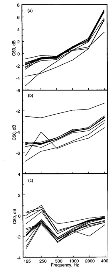
of each of the measurements are first compared in Figures 9 to 13. Each of these plots compares the results of the various measurement systems for one acoustical measure. The three parts of each plot correspond to measurements of each of the three reverberator settings. That is, part (a) is for measurements of ALEX preset 3, part (b) for preset 10, and part (c) for preset 11. Figure 9 shows Cso
measurements for each of the three reverberator settings. Similarly, Figure 10 compares Cso values; Figure I 1 compares TS values; Figure 12 compares EDT values, and Figure 13 compares RT values.
Figure 9. Comparison of 15
different measurements of octave band CS0 values for ALEX reverberator: (a) preset 3, (b) preset 10, and
(c) preset 11.
125 250 500 1000 2000 Frequency. Hz
Figure 10. Comparison of 19 different measurements of octave band Cgg values for ALEX reverberator: (a)
preset 3, (b) preset 10, and (c) preset 1 I
' ~ 5 2'50
jOO
idoo
2doo dido Frequency, HzFigure 11. Comparison of 0.14
13 different measurements
of octave band TS values for 0.1 2 ALEX reverberator: (a)
preset 3, (b) preset 10, and
0.1
(c) preset 1 I .
ffl 0.08
125 250 500 1000 2000 401
Figure 12. Comparison of
20 different measurements of octave band EDT values for ALEX reverberator: (a) preset 3, (b) preset 10, and
(c) preset 1
I.
O 125 250 500 1000 2000 4000
Figure 13. Comparison of 21 different measurements of octave band RT values for ALEX reverberator: (a) preset 3, (b) preset 10, and
(c) preset 11.
In most of these plots, the majority of the data sets cluster quite closely together and a small number of measurements are more divergent from the central trend. For example, Figure 9(a) includes 15 sets of Cso measurement results. Four of these sets of results seem to diverge significantly from the central trend.
However, the other 11 sets of results cluster quite tightly together. In some cases the scatter seems greater, but this is usually due to a larger number of sets of data being present. For example, Figure 10(b) seems to exhibit more scatter. In this case, 6 of the 19 sets of Cso values seem to signif~cantly differ from the central trend.
Two parts of these 15 plots in Figures 9 to 15 do exhibit somewhat different overall trends. In Figure 9(c), the C50 values seem to group into two separate clusters. This is particularly true in the lower three octave bands. The EDT comparisons of Figure 12(a) are unique in that the spread among the various results is quite large and these differences are greatest at high frequencies. These two special cases will be considered further later.
To better illustrate how the results of each measurement system differ from the central trend, individual results were plotted as the differences from the "best" average values. These "best" average values were calculated from the results that clustered to&ther well for all of the five different acoustical measures included in this section. The resulting "best" average values are given in Table 7 and are taken to be the best indication of the correct value for each measurement. The standard deviations of the tightly clustering results were also calculated and are given in Table 8. These standard deviations indicate the typical spread of the better results about the "best" average values. It is suggested that the results of better measurement systems should fall within k2 of these standard deviations about the "best" average values. Thus, the following plots compare the
differences of individual measurements from the "best" average values with the calculated standard deviations of the clustering results. In each figure, the shaded area indicates +1 standard deviation from the "best" average values and the dashed lines indicate 5 2 standard deviations from the better results.
To make comparisons easier, all plots of the same acoustical quantity and reverberator setting were normally plotted with the same verticle scale. In a few cases this was not possible because some results deviated further from the mean trend. In some cases an occasional data point was allowed to go off scale. In other cases with larger deviations from the mean trend, an expanded verticle scale was used.
Frequency, Hz ALEX
Measure preset 125 250 500 loo0 2000 4000
G o ,
a3 03 -1.907 -0.800 -0.648 1.002 2.235 6.983 10 -5.125 -5.104 -4.648 -3.900 -3.672 -2.570 11 -1.422 -0.107 -2.076 -1.298 -0.645 -0.323csa,
dB 03 -1.083 -0.155 0.310 1.718 2.910 7.591 10 -4.743 -4.542 -4.141 -3.101 -3.041 -2.026 11 1.272 3.278 0.527 1.830 1.805 2.090 TS, s 03 0.1215 0.0965 0.0932 0.0801 0.0642 0.0294 10 0.1868 0.1662 0.1713 0.1582 0.1547 0.1404 11 0.0962 0.0814 0.0961 0.0898 0.0857 0.0516 EDT, s 03 1.877 1.550 1.660 1.919 1.771 2.479 10 2.343 2.149 2.223 2.246 2.239 2.202 11 1.416 1.267 1.414 1.402 1.430 1.425 RT, s 03 1.192 1.262 1.260 1.266 1.195 1.306 10 1.950 2.013 2.054 2.053 2.01 1 1.837 11 1.264 1.335 1.374 1.404 1.393 1.339Table 7. "Best" average data (averages of benerjimmng data) for each setting of the ALEX reverberator.
Frequency, Hz
ALEX
Measure preset 125 250 500 loo0 2000 4000
Cso, dB 03 0.279 0.089 0.099 0.097 0.127 0.114 10 0.109 0.079 0.067 0.069 0.053 0.066 11 1.144 0.668 0.389 0.238 0.189 0.168 Cso, dB 03 0.212 0.091 0.130 0.090 0.117 0.116 10 0.325 0.285 0.143 0.166 0.130 0.117 11 0.443 0.211 0.159 0.121 0.088 0.064 TS, s 03 0.0062 0.0026 0.0021 0.0016 0.0013 0.0009 10 0.0051 0.0038 0.0021 0.0017 0.0012 0.0020 11 0.0061 0.0019 0.0022 0.0028 0.0011 0.0011 EDT, s 03 0.101 0.057 0.221 0.163 0.191 0.812 10 0.025 0.014 0.020 0.034 0.012 0.070 1 1 0.014 0.029 0.014 0.011 0.029 0.060 RT, s 03 0.039 0.031 0.021 0.025 0.025 0.063 10 0.019 0.030 0.037 0.025 0.046 0.059 11 0.019 0.101 0.010 0.012 0.010 0.010
Table 8. Standard deviations of the better results about the "best" averaae data for each setting of the ALEX reverberator.
As an initial example, Figure 14(a) compares the differences of Cso values from the "besf' average values for measurements from measurement svstems A and B (RAMSoft-I1 and RAMSoft-3). For this example, most of the octave band measurements are within f 1 standard deviation of the "best" average values and all results are within rt2 standard deviations of the "best" average results.
Figures 14(b) and (c) show the differences of Cso values from the "best" average values for the ALEX reverberator presets 10 and 11 for the RAMSoft-II and RAMSoft-3 measurement system results. All results are within rt2 standard deviations of the "best" average values. However, the standard deviations of the better results about the "besf' average values are considerably greater for ALEX
memory setting 11 than for the other two settings shown in Figure 14(c). This is due to the greater spread of the Cso values shown in Figure 9(c) for this ALEX reverberator preset 11 case.
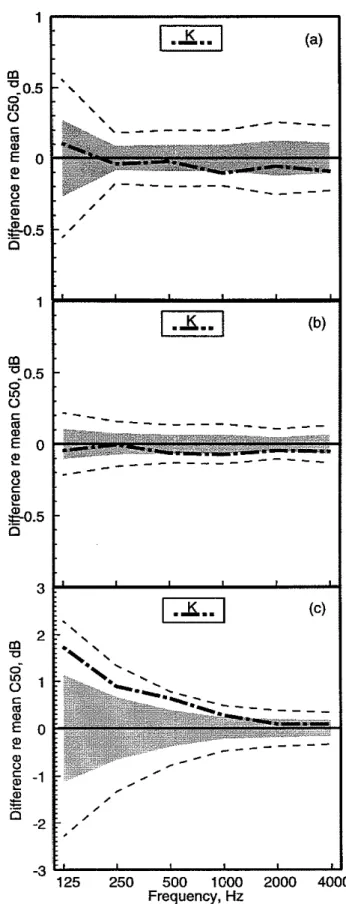
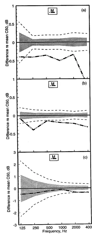
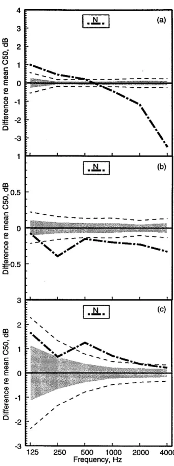
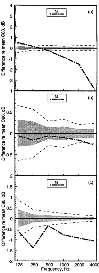
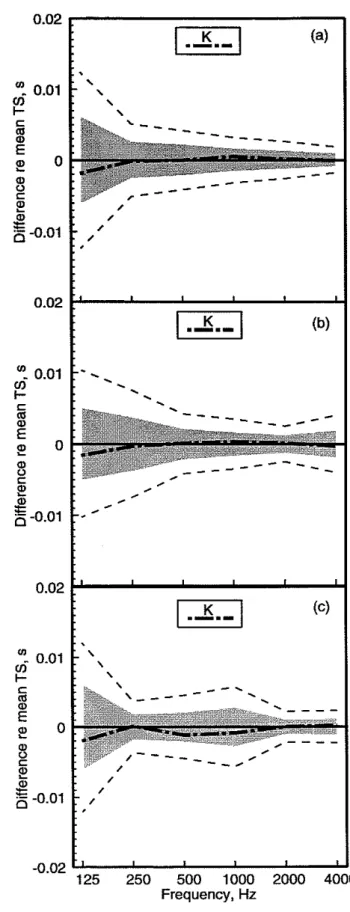
Figures 14 to 75 show the differences of the results for all measurement groups from the "best" average values. These provide each measurement group with detailed comparisons of their measurement system with the "best" average values and should be useful for identifying problems with each measurement system. To reduce the number of graphs, some related measurement results are combined on a single graph. Each figure contains three parts corresponding to the results from the three reverberator preset settings. Thus, each figure shows all results for one acoustical quantity and one(or two) measurement system(s). Figures 14 to 23 show the differences for CS0 values; Figures 24 to 37 show the differences for Cso values; Figures 38 to 47 show the differences for TS values; Figures 48 to 61 show the differences for EDT values; and Figures 62 to 75 show the differences for RT values.
Figure 14. Comparison of 1 differences of measured
octave band C50 values
from "best" average m
values for measurement
?
0.50
systems A and B
(RAMSoft-11 and
S
Cm
RAMSoft-3):
(a) ALEX preset 3,
2
P! 0 (b) ALEXpreset 10, and8
(c) ALEX preset 11. c 9-3
1 '
L125 250 500 1000 2000 40
Figure 15. Comparison of differences of measured octm$e band Cso values from "best" avmage
values for measurement system C: (a) ALEX p m e t 3, (b) ALEXpreset 10, und (c) ALEX preset 11. -3
1 '
I
125 250 500 1000 2000 4000 Frequency, HzFigure 16. Comparison of differences of measured octave band Cm values from "best" average
values for measurement systems D and E:
(a) ALEX preset 3, (b) ALEXpreset 10, and (c) ALEX preset I I .
-"
125 250 500 1000 2000 4000
Figure 17. Comparison of differences of measured octave band Cso values from "best" average
values for measurement systems F and G: (a) ALEX preset 3, (b) ALlTXpreset 10, and (c) -preset 1 I . 4 F G
- - - -
.-..-
(a) 3 -3 F ' I 125 250 500 1000 2000 4000 Frequency, HzFigure 18. Comparison of differences of measured octave band C f o values from "best" average
v a h w for measurement system K:
(a) ALEX preset 3, (b) ALEX preset 10, and (c) ALEX preset I I .
-3 € 1
I
125 250 500 1000 2000 4000
Figure 19. Comparison of differences of measured octave band Cso values from "best" average
values for measurement system M:
(a) ALEX preset 3, (b) ALEXpreset 10, and (c)
ALM
preset 11.-3 k '
125 2% 500 1000 2000 4000
Figure 20. Comparison of differences of measured octave band Cso values from "best" average
values for measurement system N: (a) ALEXpreset 3, (b) ALEXpreset 10, and (c) ALEX preset 11. -3 125 250 500 1000 2000 40 Frequency, Hz 1
Figure 21. Comparison of 1 differences of measured
octave band Cfo values
from "best" average m
values for measurement 'q0.5
0
system 0: LD
0
(a) ALEX preset 3,
(6) ALEXpreset 10, and
FJ
(c) ALEXpreset 11.i!
m
08
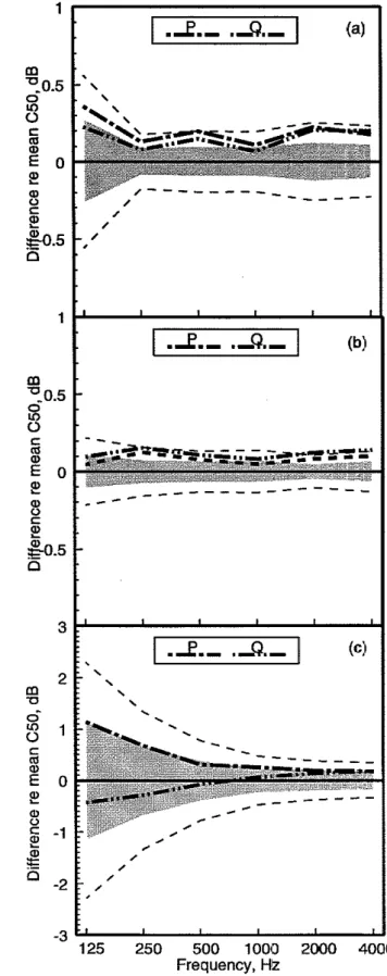
C m 125 250 500 1000 2000 4C Frequency, HzFigure 22. Comparison of differences of measured octave band C50 values from "best" average
values for measurement systems P and Q: (a) ALEX preset 3, (b) ALEXpreset 10, and
(c) ALEX preset I I .
-3
F '
125 250 500 1000 2000 4000
Figure 23. Companion of 4
differences of measured
octave band Cso values 3 from "best" average
values for measurement
%
2systems R and S:
(a) ALEX preset 3.
8
s 1(b) ALEX preset 10, and
3
(c) ALEX preset 11. E
e
01
125 250 500 1000 2000 40
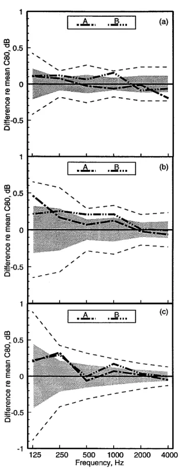
Figure 24. Comparison of differences of measured octave band Cm values from "best" average
values for measurement systems A and B
(RAMSoft-I1 and RAMSoft-3): (a)
ALM
preset 3,(b) ALEX preset 10, and (c) ALEX preset I I .
/
I
125 250 500 1000 2000 4000
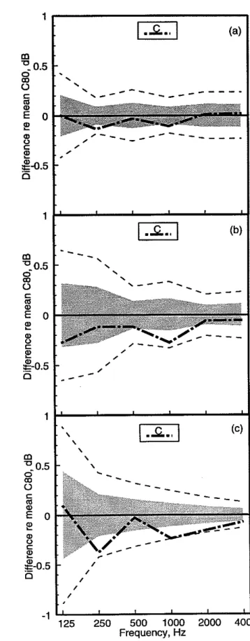
Figure 25. Comparison of differences of measured octave band Cm values from "best" average
values for measurement system C: (a) ALEXpreset 3, (b) ALEXpreset 10, and (c) ALEXpreset 1 I . / / 125 250 500 1000 2000 4C Frequency, Hz
Figure 26. Comparison of differences of measured octave band Cm values from "best" average
values for measurement systems D and E: (a) tUEX preset 3, (b) ALEX preset 10, and (c) ALEX preset 11.
Figure 27. Comparison of differences of measured octave band Cm values from "best" average
values for measurement system F and G: (a) ALEX preset 3,
(b) ALEX preset 10, and (c) ALEX preset I I .
125 250 500 1000 2000 400
Frequency, Hz
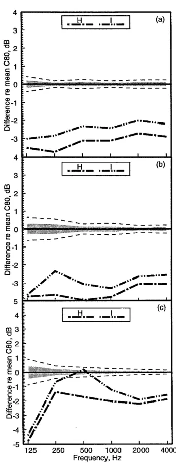
Figure 28. Comparison of differences of measured octave band Cso values
from "best" average values for measurement systems Hand 1: (a) ALEX preset 3, (b) ALEXpreset 10, and (c) ALEX preset 11. -. A 125 250 500 1000 2000 4000 Frequency. Hz
Figure 29. Comparison of differences of measured octave band Cw values from "best" average
values for measurement system J:
(a) ALEX preset 3, (b) ALEXpreset 10, and (c) ALEX preset 11. Page 43 - 8 125 250 500 1000 2000 4000 Frequency, Hz
Figure 30. Comparison of 1
differences of measured octave band Cgg values from "best" average
values for measurement
%
0- 0.5
system K: m 0
(a) ALEX preset 3,
z!
(b) ALEXpreset 10, and a
( c ) A m p r e s e t I I . E
F
0125 250 500 1000 200C 40 Frequency, Hz
Figure 31. comparison of differences of measured octave band Cm values from "best" average
values for measurement wstem M:
(a) ALEX preset 3,
(b) ALEXpreset 10, and (c) ALEX preset 11.
-1 1 ' I
125 250 500 1000 2000 4000
Figure 32. Comparison of differences of measured octave band C80 values from "best" average
values for measurement system
N:
(a) ALEX preset 3, (b) ALEXpreset 10, and (c)
ALEX
preset 11.I
125 250 500 1000 2000 4000 Frequency. Hz
Figure 33. Comparison of 1 differences of measured
octave band Cm values
from "best" average m
values for measurement 0.5
system 0:
(a) ALEX preset 3,
s
s
(b) ALEX preset 10, Md (c) ALEX preset 11.
E
0 / -1 ' 1 125 250 500 1000 2000 40 Frequency, Hz 0Figure 34. Comparison of differences of measured octave band Cgg values from "best" average
values for measurement systems P and Q:
(a) ALEX preset 3, (b) ALEX preset 10, and
(c) ALEX preset 11.
' 125 250 500 1000 2000 4000
Figure 35. Comparison of differences of measured octave band C80 values from "best" average
values for measurement systems R and S: (a) ALEX preset 3, (b) ALEX preset 10, and (c)
ALEX
preset 11./
I
125 250 500 1000 2000 4000
Figure 36. Comparison of differences of measured octave band CW values from "best" average
values for measurement system T:
(a) ALEX preset 3,
(b)
ALEX
preset 10, and(c) ALEX preset 1 I .
Figure 37. Comparison of differences of measured octave band Cgg values from "best" average
values for measurement system U:
( a ) U p r e s e t 3, (b) ALEXpreset 10, and (c) ALEXpreset 1 I .
Figure 38. Comparison of differences of measured octave band TS values from "best" average
values for measurement systems A and B
(RAMSofr-IZ and RAMSoft-3): ( a ) ALMpreset 3, (b) ALEX preset 10, and (c) ALEX preset I I .
-0.02
125 250 500 1000 2000 4C
Figure 39. Comparison of 0.02
differences of measured octave band TS values from "best" average
U)
values for measurement V) -0.01
systems D and E: c C ( a ) ALEXpreset 3, m (b) ALEXpreset 10, and
i!
(c) ALEX preset 11. g! 05
1
(a) 1 1 I 125 250 500 1000 2000 4000 Frequency, HzFigure 40. Comparison of differences of measured octave band TS values from "best" average
values for measurement system G:
(a) ALEX preset 3, (b) ALEX preset 10, and (c) ALEX preset 11. U) -0.01 (I)
+
125 250 500 1000 2000 4001 Frequency, Hz 3Figure 41. Comparison of differences of measured octave band TS values from "best" average
values for measurement system J: (a) A m p r e s e t 3, (b) ALEXpreset 10, and (c) ALEX preset I I . (c) -0.02 125 250 500 1000 2000 4000 Frequency, Hz
Figure 42. Comparison of diSferences of measured octave band TS values from "best" average
values for measurement system K:
(a) ALEX preset 3, (b) ALEXpreset 10, and (c)
ALEX
preset 11.25 250 500 1000 2000 4( Frequency, Hz
Figure 43. Comparison of differences of measured octave band TS values from "best" average
valws for measurement system M:
(a) ALEX preset 3, (b) ALEXpreset 10, and (c) ALEX preset 11.
25 250 500 1000 2000 4c Frequency, Hz
Figure 44. Comparison of differences of measured octave band TS values from "best" average
values for measurement system N:
(a) ALEX preset 3, (b) ALEXpreset 10, and
(c) ALXXpreser 1 I .
Frequency, Hz
Figure 45. Comparison of 0.02
differences of measured octave band TS values from "best" average
w
values for measurement -0.01
fn
system 0: I-
(a)
ALM
preset 3, C m(b) ALEXpreset 10, and
z
(c)ALM
preset 1 I .P
a
8
c -0.02 f ' J 125 250 500 1000 2000 400 Frequency, HzFigure 46. Comparison of differences of measured octave band TS values from "best" average
values for measurement systems P and Q: (a) ALEX preset 3. (b) ALEX preset 10, and (c) ALMpreset 11. 0.02
.-.- .-..-
7
1
(a) -0.02 f'
I
125 250 500 1000 2000 400 Frequency, Hz 0Figure 47. Comparison of 0.03
differences of measured octave band TS values
from "best" average 0.02
U)
values for measurement mi
systems R and S:
t
0.01(a)
ALM
preset 3, m(b) ALEXpreset 10, and
g
(c) ALEXpreset 11. e! a, Os
125 250 500 1000 2000 400C
Figure 49. Comparison of differences of measured octave band EDT values from "best" average
values for measurement system C:
(a) ALEX preset 3,
(b) ALEXpreset 10, and (c) ALEXpreset 11.
- - -
Figure 50. Comparison of differences of measured octave band EDT values from "best" average
values for measurement systems D and E: (a) ALMpreset 3, (b) ALEX preset 10, and (c) ALEXpreset 11.
-0.3
125 250 500 1000 2000 4000
Figure 51. Comparison of &zerences of measured octave band EDT values from "best" average
values for measurement systems F and G: (a) ALEXpreset 3,
(b) ALEX preset 10, and
(c) ALEX preset 11.
125 250 500 1000 2000 40
Figure 52. Comparison of
differences of measured 2
octave band EDT values I C . I
from "best" average
U )
values for measurement i 1
systems Hand I:
b
W(a) ALEX preset 3,
5
0.5(b) ALEX preset 10, and
(c) ALEX preset 11. g! 0 m -0.5
$
E -1 0-"."
125 250 500 1000 2000 4000 Frequency, HzFigure 53. Comparison of differences of measured octave band EDT values from "best" average
values for measurement system J:
(a) ALEX preset 3, (b) ALEX preset 10, and (c) ALLZ preset 11.
-0.3 ' I 125 250 500 1000 2000 4000
Figure 54. Comparison of differences of measured octave band EDT values from "best" average
vahes for measurement system
K:
(a) ALEXpreset 3, (b) ALEX preset 10, and (c) ALEX preset 11.
-0.3
'
I125 250 500 1000 2000 400
Figure 55. Comparison of differences of measured octave band EDT values from "best" average
valuer for measurement system M:
(a) ALEXpreset 3, (b) ALEX preset 10, and (c) ALEX preset 11.
-0.3
125 250 500 1000 2000 40C
Figure 56. Comparison of differences of measured octave band EDT values from "best" average
values for measurement system
N:
(a) ALEX preset 3, (b) ALEX preset 10, and
(c) ALEXpreset 11.
-0.3
'
I125 250 500 1000 2000 4000
Figure 57. Comparison of diftermces of measured octave band EDT values
from
"best" averagevaluesjbr measurement system 0:
(a) ALEX preset 3,
(b) ALEX preset 10, and (c) ALLXpreset 11.
-0.3 '
I
125 250 500 1000 2000 40(
Figure 58. Comparison of differences of measured octave band EDT values from "best" average
values for measurement systems P and Q: (a) ALEXpreset 3, (b) ALEX preset 10, and (c) U p r e s e t 1 I .
-0.3
'
I I125 250 500 1000 2000 4000
Figure 59. Comparison of differences of measured octave band EDT values from "best" average
values for measurement systems R and S: (a) ALEXpreset 3, (6) ALEX preset 10, and (c) ALEX preset I I .
-0.3
'
J 125 250 500 1000 2000 4000Figure 60. Comparison of differences of measured
octave band EDT values 1.5
from "best" average U)
values for measurement
system T:
n
W (a) ALEXpreset 3, 0.5 (6) ALEXpreset 10, and 0 (c) ALEX preset 11. 2__--.
m 93.5 e! m z -1 n \ -0.3'
125 250 500 1000 200C 4( Frequency, HzFigure 61. Comparison of differences of measured octave band EDT values from "best" average
values for measurement system U:
(a) ALEX preset 3, (b) ALEX preset 10, and (c) ALEXpreset I I .
-0.3 ' I 125 250 500 1000 2000 4000
Figure 62. Comparison of differences of measured octave band RT values from "best" average
values for measurement systems A and B
(RAMSoft-I1 and RAMSoft-3): (a) ALM preset 3, (b) ALEX preset 10, and (c) ALEX preset I I .
-0.2