Cache-oblivious dynamic search trees

Cache-Oblivious Dynamic Search Trees

by

Zardosht Kasheff

Submitted to the Department of Electrical Engineering and Computer

Science

in partial fulfillment of the requirements for the degree of

Masters of Engineering in Computer Science and Engineering

at the

MASSACHUSETTS INSTITUTE OF TECHNOLOGY

June 2004

@Zardosht Kasheff, 2004.

rho **who" DOW 10b

MW

Pwo stopoducenpowt

itbutmW

PAt

OMW01

pubfcr pae

and

obcwop*c

-

C

#*tw"*s

WO

TInr

~wgo

or ih Poe

. ..

uepartment of Electrical Engineering and Computer Science

May 24, 2004

i

Certified by ..

. . . .. . . ... . ... .. .N. ... . .. . . .

Dr. Bradley Kuszmaul

Research Scientist

7

Thesis Supervisor

Accepted by ...

.

/ ...

Arthur C. Smith

Chairman, Department Committee on Graduate Students

MASSACHUSETTS INSTMiUTE.

OF TECHNOLOGY

JURL 2 2004

Author.

_.t

Cache-Oblivious Dynamic Search Trees

by

Zardosht Kasheff

Submitted to the Department of Electrical Engineering and Computer Science on May 24, 2004, in partial fulfillment of the

requirements for the degree of

Masters of Engineering in Computer Science and Engineering

Abstract

I have implemented a cache-oblivious dynamic search tree as an alternative to the ubiquitious B-tree. I use a binary tree with a "van Emde Boas" layout whose leaves point to intervals in a "packed memory structure". We refer to the data structure as a Tree. The COB-Tree supports efficient lookup, as well as efficient amortized insertion and deletion. Efficient implementation of a B-tree requires understanding the cache-line size and page size and is optimized for a specific memory hierarchy. In contrast, the COB-Tree contains no machine-dependent variables, performs well on any memory hierarchy, and requires minimal user-level memory management. For random insertion of data, my data structure performs 7.5 times faster than the Berkeley DB and 3 times faster than a memory mapped implementation of B-trees. The packed memory array of the COB-Tree maintains data in sorted order, allows sequential reads at high speeds, and data insertions and deletions with few data writes on average. In addition, the data structure is easy to implement because I employed memory mapping rather than explicit file operations.

Thesis Supervisor: Dr. Bradley Kuszmaul Title: Research Scientist

Acknowledgments

I would like to thank Dr. Bradley Kuszmaul and Professor Michael Bender, for working

closely with me on all aspects of my project and thesis. Their help and guidance made this work possible. I would also like to thank Dr. Kuszmaul for implementing a memory-mapped B-tree to compare to my COB-Tree. I would like to thank Professor Charles Leiserson for helpful discussions on my project, thesis, and presentations of my work.

I would like to thank the other students of the Supercomputing Technologies group at the Computer Science and Artificial Intelligence Laboratory at MIT: Kunal Agrawal, Elizabeth Basha, John Danaher, Jeremy T. Fineman, I-Ting Angelina Lee, Sean Lie, Tim Olsen, Siddhartha Sen, and Jim Sukha. All provided helpful discussions and feedback throughout the year.

I would like to thank my family and friends, whose love and support have motivated me all of my life.

Finally, I would like to thank Professor Albert Meyer and Dr. Eric Lehman for allowing me to assist them in teaching Mathematics for Computer Science, thus funding my education for the last semester. Their understanding and flexibility helped allow me to balance research and teaching very effectively.

Contents

1 Introduction

2 Description

2.1 B-trees . . . . 2.2 Cache-Oblivious Model . . . .

2.3 Cache-Oblivious Dynamic Search Trees . .

2.3.1 Static Cache-Oblivious Binary Tree

2.3.2 Packed Memory Structure . . . . .

2.3.3 Combined Data Structure . . . .

2.3.4 Related Work. . . . .

3 Results

3.1 Comparing COB-Trees and B-Trees . . . . 3.2 Asymptotic Behavior of COB-Tree . . . . 3.2.1 Random Insertion Pattern . . . . .

3.2.2 Insertion-at-Head Pattern . . . . .

4 Static Cache-Oblivious Binary Tree Implementation

4.1 Algorithm to Convert Breadth-First Index to van Emde Boas Index . . . . . 4.2 Evaluating Heights of Subtrees . . . . 4.3 Evaluating New Depth and Number of Preceding Nodes . . . . 4.4 Evaluating Breadth-First Index of Recursive Case . . . . J 13 15 . . . . 15 . . . . 18 . . . . 19 . . . . 19 . . . . 20 . . . . 22 . . . . 22 25 . . . 26 . . . 27 . . . 27 . . . 28 35 38 38 40 41

5 Packed Memory Structure Implementation 43

5.1 Data Representation ... ... 43

5.2 Insertion . . . .. . . .. 44

5.3 Rebalancing . . . . 46

5.3.1 Simple Rebalancing Algorithm . . . . 47

5.3.2 Read-Efficient Algorithm . . . . 47

5.3.3 Write-Efficient Algorithm . . . . 50

5.3.4 Partially Correct Efficient Algorithm . . . . 51

6 Conclusion 53 6.1 Future Work. . . . . 53

6.2 Future Vision . . . . 54

List of Figures

2-1 Two-Level Memory Hierarchy with a disk block size of B and memory size of

M... ... ... 16

2-2 B-tree with capacity of 3 keys per node. . . . . 17 2-3 van Emde Boas example in general and of height 5. Figure taken from

[7].

. 20 2-4 An example of the packed memory structure containing the values 1 through

16. The array contains 8 sections. The binary tree is labeled with a

breadth-first layout along with the bit representations of the layout. The sections are labeled below the array. The numbers in bold italics in the nodes are values

held by the node. . . . . 23

3-1 Average time for insertion with random insertion pattern . . . . 28 3-2 (Average time for insertion)/(lg2(number of elements)) with random insertion

pattern. . . . . 29 3-3 Average time for insertion with insertion-at-head pattern. . . . . 29

3-4 (Average time for insertion)/(g 2 (number of elements)) with insertion-at-head pattern. . . . . 30 3-5 Average number of data moves with random insertion pattern. . . . . 30 3-6 Average number of data moves with insertion-at-head pattern. . . . . 31 3-7 (Average number of data moves)/(lg2(number of elements)) with

insertion-at-head pattern. . . . . 31 3-8 Average rebalancing sum with random insertion pattern. . . . . 32 3-9 Average rebalancing sum with insertion-at-head pattern. . . . . 32

U-3-10 (Average rebalancing sum)/(g2(number of elements)) with insertion-at-head pattern . . . . . 33

4-1 van Emde Boas and Breadth First indices on tree of height 5. van Emde Boas indices are in black letters. Breadth first indices are in white letters. Figure taken from [7]. . . . . 36

4-2 General method of van Emde Boas layout. In memory, the subtrees A, B1, B2,.. ., B,

are recursively laid out in order. Figure taken from [7]. . . . . 39

4-3 A partial diagram of a tree with height 7 in breadth-first order. The seven nodes at the top three depths make up subtree A of the van Emde Boas layout. The subtree with root node 11 forms subtree B4 of the van Emde Boas layout. 41 5-1 The initial state of the array before rebalancing begins. The array has four

sections, each with a capacity of four elements . . . . . . 48

5-2 The state of the array after all elements have been crunched to the left. . . . 48

5-3 The final state of the array after elements have been redistributed from the crunched array. . . . . 48 5-4 The initial state of the array before rebalancing begins. The array has four

sections, each with a capacity of four elements. . . . . 49

5-5 The state of the array after section 1 is crunched towards Section 2. Sections

3 and 4 remain to be crunched. . . . . 50 5-6 The state of the array after Sections 3 and 4 are crunched towards section 2. 50 5-7 The initial state of the array before rebalancing begins. The array has four

sections, each with a capacity of four elements. . . . . 51 5-8 The state of the array after all right moving elements have been relocated. . 52 5-9 The final state of the array after left moving elements 1, 10, and 18 have been

m oved as well. . . . . 52 I.

List of Tables

3.1 Time needed to insert 40,000 520 byte keys into an empty database, in seconds. 26

3.2 Time needed to insert 160,000 520 byte keys into an empty database, in seconds. 26 4.1 Values of temp and val in executing hyperfloor(25). . . . . 39

Chapter 1

Introduction

For decades, B-trees [2, 11] have been the predominant dictionary data structure. The B-tree is a k-ary tree where k is selected such that each node of the B-tree is the size of a block of disk. B-trees minimize the number of disk block transfers from disk to main memory needed to traverse down a path of the tree. Although efficient, B-trees require the programmer to experimentally tune the value of k on any machine used. Because machines are complex, finding the optimal k is a complex task that may even be impossible.

This thesis presents the implementation and testing of an alternative data structure that requires no such tuning, a "cache-oblivious" dynamic search tree. We refer to this data structure as a COB- Tree. The data structure is cache-oblivious because the implementation does not depend on any machine dependent variables such as disk block size or main memory size. Still, the COB-Tree has been proven to perform within a constant factor of the least number of memory transfers possible between any consecutive levels of memory.

The COB-Tree, presented by Bender, Demaine, and Farach-Colton [7], has two compo-nents: a static cache-oblivious binary tree and a loosely packed array. Data is kept in sorted order in the array. The leaves of the binary tree correspond to certain sections of the array. To insert elements, we search the tree to find the appropriate section and try to insert the element while moving as few other elements as possible. Infrequently, when sections of the array become too dense, we redistribute a larger portion of the array evenly.

The COB-Tree is tested on large test cases, comparing performance with the standard solution, B-trees, and analyzing asymptotic properties. One set of experiments involving disk access shows comparisons between the cache-oblivious search tree and B-trees. I compare performances using two insertion patterns and analyze results. When inserting elements with a random insertion pattern, the COB-Tree performs 3 times faster than a memory-mapped implementation of B-trees and 7 times faster than the Berkeley DB [23]. When inserting elements repeatedly into the same location, the COB-Tree performs only 3.5 times worse than both memory mapped B-trees and the Berkeley DB. Because we require data to remain in sorted order on disk, we expected much worse. Another set of experiments analyzes asymptotic runtime behavior of the cache-oblivious search tree. I compare experimental behavior of runtime, number of data moves, and data distribution costs with costs derived

by theoretical analysis of the data structure on simple memory models.

I present details of the implementation of the COB-Tree, including arguments for why the implementation is efficient. The binary tree is an array in memory with a non-intuitive layout, the van Emde Boas layout. I implemented a function that converts indices from a simple layout, the breadth-first layout, to the layout of the cache-oblivious binary tree. Thus, the details of the cache-oblivious layout are abstracted from the programmer. The programmer, using the function, may program as though he is using the simple breadth-first layout. I present details on implementing each phase of the insertion algorithm, along with reasons for each non-trivial algorithmic decision. I show how the data is stored in memory using a single-level store. Finally, I present several solutions for the most work-intensive operation, redistributing many elements across the array.

The rest of this thesis is organized as follows. Chapter 2 describes, in detail, the cache-oblivious dynamic search tree, as developed over the last few years. We review the perfor-mance model used in previous literature to analyze cost and summarize theoretical arguments for why the tree performs well. Chapter 3 presents experimental results. Chapter 4 presents details of the implementation of the static cache-oblivious binary tree. Chapter 5 describes how to implement the loosely packed array.

Chapter 2

Description

We focus on the problem of creating a data structure that supports efficient data scans, searches, insertions, and deletions. The traditional solution, B-trees, has limitations. B-trees perform sub-optimally on machines with complex memory hierarchies and employ machine dependent variables such as block size of disk. A simple and efficient alternative data struc-ture, the COB-Tree, has been shown to perform asymptotically optimally on any memory hierarchy while not depending on any machine dependent variables. This chapter explains why, while Chapter 3 provides experimental results of the COB-Tree, and Chapters 4 and 5 present implementation details.

This chapter is organized as follows. Section 2.1 describes B-trees and their limitations. Section 2.2 presents the cache-oblivious model, which helps explains why COB-Trees theo-retically perform well. Section 2.3 introduces the COB-Tree.

2.1

B-trees

B-trees are designed to perform optimally on the Disk Access Machine (DAM) Model [11, an idealized two-level memory model consisting of a CPU, main memory of size M, and disk, broken into blocks of size B. Unlike the Random Access Memory model, which assumes constant access time for all memory locations, the DAM model assumes memory transfers

of blocks from disk to main memory to be the most time consuming operation. Thus, cost is measured in memory transfers. Figure 2-1 shows an example of the two-level memory hierarchy. CPU H- B--main memory MIB D

S

K

Figure 2-1: Two-Level Memory Hierarchy with a disk block

M.

size of B and memory size of

The B-tree works as follows. The B-tree nodes has degree proportional to the block size,

B. Each node of size B holds as many pairs of keys and pointers as it may. The B-tree has

uniform depth and is nearly balanced. Traversing an edge down the tree reduces the search space by a factor proportional to 1/B. Thus, B-trees perform data searches in 0(1 + log N) memory transfers. An information-theoretic argument proves this bound is asymptotically optimal. Figure 2-2 shows an example of a B-tree.

The biggest shortcoming of B-trees is that they are optimized for only an idealized two-level memory hierarchy where B is fixed. Real memory hierarchies have multiple two-levels and are more complex than the two-level memory hierarchy. Machines today have multiple levels of memory including registers, level-1 cache, level-2 cache, main memory, and disk. When

50I

0o0 1

40

44

481

60

0

3035

4142143

55[7]

Figure 2-2: B-tree with capacity of 3 keys per node.

using a multilevel memory hierarchy, the programmer of a B-tree must decide which level of memory is the bottleneck and optimize accordingly. To program efficiently under a multilevel memory hierarchy requires the user to consider multiple block sizes B1, B2, . . . , B,,. To create a tree that is aware of these blocks sizes, aware of the number of memory levels, and performs optimally is very complex, at best.

Define the effective block size to be the value, B, B-trees should use as the size of a node to maximize performance. This value, if it even exists, may differ from the actual block size. Consider the effective block size of disk, the memory level for which most B-trees optimize. The disk consists of not only blocks, but tracks and cylinders as well. Disks engage in prefetching, that is, reading an entire track of data when only a disk block is requested. Tracks near the center of the platter are smaller than tracks near the end, thus the effective block size varies throughout the disk. The time to perform a seek to a track may vary by an order of magnitude, ranging from a track-to-track seek to a full seek. Remapped Bad Sectors change the effective block-transfer size and transfer cost. The Translation Lookaside Buffer complicates things. As a result of all of these complications, finding the optimal value, B, to optimize a B-tree for disk, is very difficult and may even be impossible.

Most of these effects can be mitigated by improving data locality. Thus, many database-management systems heuristically group logically close disk blocks physically near each other on disk [12, 16, 17, 19, 22]. Alternatively, many authors build B-trees that are optimized for

more detailed models of the memory hierarchy, typically for the DAM model extended to three levels, disk, memory, and cache. Such modified B-trees consist of cache-line B-trees at each node of a larger disk-block B-tree [3, 4, 7, 10]. Indeed, these 2-parameter B-trees have been shown to perform better than 1-parameter B-trees [10] by reducing cache misses.

These 2-parameter B-trees do not model certain disk properties such as prefetching, track size diversity, track locality, work load effects, disk cache. Even when generalizing 2-parameter B-trees to k-parameters B-trees, address such issues is difficult, because such memory effects are unpredictable and difficult to measure. Finally, it has been shown that the improvement given by increasing k is limited at least in theory [3].

2.2

Cache-Oblivious Model

Before presenting our alternative data structure, we present the cache-oblivious model [13, 20]. Like the DAM model, the cache-oblivious model is based on the on the Ideal Cache

Model [14, 201. In the Ideal Cache Model, the cache of size M is divided into MIB blocks of

size B. The cache is a fully associative cache which can store an arbitrary block of memory into any "slot" of cache. The cost of transferring data from main memory to cache is the most expensive operation. Like the DAM model, a simple, and often accurate, performance measure of algorithms is to count the number of memory transfers of blocks from main memory to cache. Although the model assumes an unrealistic fully-associative cache, the model may be simulated with actual hardware with a constant factor of overhead [14]. Thus, results proved on this model are applicable to pairs of levels in the multilevel memory hierarchy.

Unlike the DAM model, the cache-oblivious model proves results on complex multilevel-memory hierarchies. Algorithms using the cache-oblivious model are not dependent on the block size B and main memory size M. If an algorithm performs optimally on the cache-oblivious model, the algorithm performs asymptotically optimally on any unknown multilevel memory hierarchy. From this we define two types of algorithms. Optimal algorithms execute

within a constant factor of the least possible number of memory transfers possible.

Opti-mal cache-aware algorithms are optiOpti-mal algorithms aware of the memory parameters of the

machine the algorithm is run on, M and B. Optimal cache-oblivious algorithms perform op-timally with no knowledge of M and B. We refer to these as cache-aware and cache-oblivious algorithms respectively.

2.3

Cache-Oblivious Dynamic Search Trees

The first dynamic cache-oblivious B-tree was proposed by Bender, Demaine and Farach-Colton [7]. Simplified alternatives include [6, 8, 9, 21]. Some of these simplifications have been evaluated experimentally for small data sets [8, 9, 18, 21], but there has been relatively little attempt to analyze the performance of cache-oblivious search structures on very large sets, where disk performance dominates.

We implement two data structures, a static cache-oblivious binary tree [20] and a packed memory structure [7]. When combined, they form a COB-Tree.

2.3.1

Static Cache-Oblivious Binary Tree

The first data structure is a static binary tree with a cache-oblivious layout called a van

Emde Boas layout. In memory, the tree is an array. The layout describes a mapping of

nodes in the tree to positions in the array. Nodes are located in memory such that the tree may be traversed with 0(1 + log (N)) memory transfers, which is asymptotically optimal [7].

Definition of van Emde Boas Layout. The tree is laid out in memory in a recursive fashion. Let h be the height of the binary tree. For simplicity, assume h is a power of 2. Let

N be the number of nodes in the tree. We divide the tree into two sections. The first section

is the "top half" containing a subtree, sharing the same root as the tree, of height h/2 with

VN

nodes. The second section is the "bottom half" containing 2h/2 subtrees of height h/2,

first layout the top half recursively. Then layout the remaining 2h/2 subtrees recursively in

order. This represents subtrees B1, B2 ... , B, in Figure 2-3. In memory, the entire subtree

A would be laid out first, followed by B1 s... , B,. We assume the binary tree is full and

balanced. If h is not a power of 2, the bottom half of the tree is chosen such that its height is a power of 2. Figure 2-3 shows the layout of a binary tree with height 5.

'0 B1 51 <I1 2 3-' <~ A Bi Bt 1- 1 1 It I' FF1 23 5 -'0 24 25 2 3103"1

VN

Figure 2-3: van Emde Boas example in general and of height 5. Figure taken from [7].

2.3.2

Packed Memory Structure

The idea behind a packed memory structure is to maintain elements of a loosely packed array in sorted order while keeping the average insertion cost low. The goal is to leave enough blank spaces in the array so that for most insertions, few elements need to be moved to accommodate the insertion. When portions of the array become imbalanced, we redistribute elements in a larger portion of the array. This happens infrequently. Bender, Demaine, and Farach-Colton show two important asymptotic bounds regarding this data structure [7]. Insertions and deletions are done with 0(1 + 1ogLN) memory transfers on average. To scan

K consecutive elements, an additional 0(1

+

K/B) memory transfers are required.

some c > 1. The remaining fraction of the array, 1 - 1/c, is blank. Let T be the size of the array. We specify T to be a power of 2 at all times. Divide T into equally sized sections of size s = 0(log2 _{T) such that s is a power of 2. This forces the number of sections to be a} power of 2 as well. Let each section be represented by a leaf of a full and balanced binary tree of depth d.

Define the portion an internal node represents to be the union of all sections represented

by the node's leaves. Thus, nodes whose two children are leaves represent two sections,

whereas the root represents the entire array. The capacity of a node is the maximum number of elements the portion can hold. The density of a node is the number of elements maintained in its portion divided by its maximum capacity.

Each node has upper and lower density threshold bounds that are a function of its depth (distance from the root). Threshold bounds of a node are boundaries for acceptable densities of the portion the node represents. Their relevance becomes clear in the algorithm for insertion and deletion described below. Let the depth of the root node of the tree be 1 and the depth of all leaves be h. For each node at an arbitrary depth d, we have desired upper and lower bound thresholds, rd and pd respectively, for the density. We say a node, k, is within threshold if and only if Pd < density(k) < rd. The densities of the root and leaves are

pi = .4, Tr = .5, Ph = .25, and rh = 1 respectively. We have tighter thresholds for nodes of smaller depth. Therefore, we preserve the property,

Ph < ph-1 < -... < P1 < r1 < 72 < - - h-1 < Th

-Thresholds for an internal node at depth i are selected such that the thresholds T1, r2, .... , rh form an arithmetic sequence. Thus, ri = ro + i(Th - -ro)/h. Similarly, p = PO - i(po - ph)/h.

Insertion The algorithm for insertion of an element i is as follows. Search the binary tree

to find the appropriate section, j, where i belongs. If the section j is within threshold, insert

node that is within threshold. Rebalance the elements in the portion, along with i, that is, evenly redistribute all elements in the ancestor's portion. Because this node has tighter threshold bounds than all of descendant nodes, the redistribution forces all descendent nodes to be within threshold. If no ancestor is within threshold, do one of two things. The density of the array is either too high or too low. If the density of the array is higher than the upper threshold of the root node, double the size of the array. If the density of the array is below the lower threshold of the root node, decrease the size of the array by half. In both cases, rebalance after resizing the array.

Deletion Upon deletion of an element i, there are two approaches. One is to find the element and perform the same threshold tests as for insertion. The other is to disregard thresholds and remove the element.

2.3.3

Combined Data Structure

The COB-Tree is similar to the data structure presented in [8]. We have a binary tree whose leaves correspond to sections (and not individual elements, as in [8]) of a packed memory structure. The binary tree has a van Emde Boas layout. Suppose the tree has N leaves and height h. The ith leaf of the tree, corresponds to the ith section of the tree. Each internal node of the tree represents a portion, the union of all sections represented by the node's leaves. The value held at each internal node is the highest value of the left child's portion.

2.3.4

Related Work.

The packed memory structure and its analysis closely follow [15]. The paper [15] considers the same problem of maintaining elements in order in an array of linear size, but in a different cost model and without the scanning requirement. The structure moves O(log2 N) amortized

elements per insertion, but has no guarantee on the number of memory transfers for inserting, deleting, or scanning. This structure has been de-amortized in [24, 25, 26] and subsequently

42=1 0

12 3=11

2 4=100

6 =101

10 6=110

14 7=111

8=1000 9=1001 10=1010 11=1t1 12=1100 13=1101 14=1110 15=1111

1

2

3

4

5

6

7

8

9 10 11 12 13 14 15 16

0=000 1=001 2=010 3=011 4=10 5=101 6=110 7=111

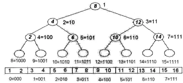
Figure 2-4: An example of the packed memory structure containing the values 1 through 16. The array contains 8 sections. The binary tree is labeled with a breadth-first layout along with the bit representations of the layout. The sections are labeled below the array. The numbers in bold italics in the nodes are values held by the node.

Algorithms

Data Query Data query is simple. To search for a particular element i, first search the binary tree to find which appropriate section i belongs. To do so, we traverse a path of the tree. If i is less than or equal to the key at a node of the tree, go left. Otherwise, go right. Figure 2-4 shows an example of the packed memory structure. Once the section is found, perform a binary search within the section.

To search for a range of elements [a, b), search for the element a in the data structure, and scan the array until an element greater than or equal to b is found. Because the data access is sequential once a is found, range queries should be very fast, operating at near 1/c times the disk drive's maximum achievable bandwidth.

Insertion/Deletion Upon insertion or deletion, use the algorithm for inserting or deleting into a packed memory structure presented above. Because the binary tree is cache-oblivious, the section

j

is found using few memory transfers.

Chapter 3

Results

Chapter 2 introduced the COB-Tree and proof that the COB-Tree theoretically performs well without the same drawbacks as B-trees. In this chapter, we experimentally analyze the performance of the COB-Tree. Chapters 4 and 5 provide implementation details of the

COB-Tree.

The experiments have two objectives: compare the performance speed of COB-Trees with B-trees on experiments involving external memory and to analyze the asymptotic behavior of COB-Trees. All experiments conducted have one of two insertion patterns:

1. Random Insertion: Each key is selected uniformly at random from the sample space

of keys.

2. Insertion-at-Head: Each key inserted is less than all previously inserted keys. This insertion pattern forces each key to be inserted at the beginning of the array.

All keys and values are 64-bit integers. The range of keys and values are [0,2"). To simulate

larger size keys, each key is padded with some number of bytes. All experiments start with 64-element arrays. Arrays are resized when needed.

The rest of the chapter is organized as follows. Section 3.1 provides results comparing COB-Trees and B-trees on experiments involving disk access. Section 3.2 shows graphs demonstrating the COB-Tree's asymptotic performance for large tests.

3.1

Comparing COB-Trees and B-Trees

Experiments were run on a Pentium II 400MHz Processor with 128MB of main memory. We inserted elements into the cache-oblivious search tree, a memory mapped implementation of B-trees, and the Berkeley DB [23]. Keys had 512 byte pads to simulate a 520 byte key. We used this small, old, machine so that we could experiments both on trees that fit in main memory and on trees that do not. In section 3.2 we use a faster machine to explore the asymptotic behavior of our data structure. We ran experiments inserting 40,000 elements and

160,000 elements using both insertion patterns presented above. Inserting 40,000 elements

takes roughly 20-40 MB of space. Therefore, the insertion may be done entirely in memory. Inserting 160,000 elements takes 80-160 MB of space, therefore forcing data to be written to disk. Table 3.1 shows insertion times for 40,000 elements. Table 3.2 shows insertion times for 160,000 elements.

COB-Tree Memory Mapped B-Tree Berkeley DB

Random Insertion 2.4s 5.03s 93.67s

Insertion-At-Head 5.2s 3.73s 10.85s

Table 3.1: Time needed to insert 40,000 520 byte keys into an empty database, in seconds.

COB-Tree Memory Mapped B-Tree Berkeley DB

Random Insertion 202s 639s 1485s

Insertion-At-Head 140s 43.6s 42.91s

Table 3.2: Time needed to insert 160,000 520 byte keys into an empty database, in seconds.

Note that for a random insertion pattern, the COB-Tree outperforms both implemen-tations of B-trees. This result is attributed to the fact that in the random insertion case, on average, many insertions occur between periods of heavy rebalancing. Thus, rebalancing occurs quite infrequently.

For the insertion-at-head pattern, the B-tree outperforms the COB-Tree by only a factor of roughly 3.5. We expected much worse. For the B-tree, this insertion pattern allows

for all relevant data elements to be stored in cache at all times. The COB-Tree requires inserting into the beginning of a sorted array every time. Given how often the COB-Tree must rebalance, performing only a factor of 3.5 worse than B-trees is quite remarkable.

3.2

Asymptotic Behavior of COB-Tree

We present graphs of the performance of the COB-Tree to show evidence of asymptotic runtime behavior. All experiments were run on a 1.4MHz AMD Opteron(tm) Processor with 16GB of main memory. Keys and values were each 8 bytes.

3.2.1

Random Insertion Pattern

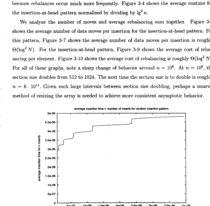
We first focus on runtime. Figure 3-1 shows the average time for random insertion. The domains of the graph demonstrating large increases in the average runtime represent times large portions of the array are rebalanced frequently. This graph demonstrates that for random insertion patterns, periods of rebalancing are infrequent, yet costly. Figure 3-2 shows the average runtime for random insertion normalized by dividing by 1g2 N. Once again, the

sharp increases are attributed to heavy rebalancing, while the dips in the graph are attributed to long areas of time of infrequent rebalancing. The graph seems to be slightly increasing, not quite demonstrating E(log2

N) amortized insertion cost the RAM model suggests.

We focus on number of moves. Define a data move to be moving of an element from one location to another within the array. Note this does not count the actual insertion of an element. Thus, it is possible to insert an element with no data moves. Figure 3-5 shows the

average number of data moves per insertion is roughly constant.

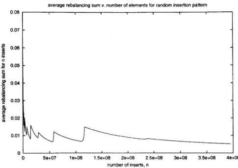
We now focus on analyzing how often we rebalance and how large the rebalances are. We calculate the sum of all the portion sizes we rebalance. Call this sum the rebalancing

sum. Figure 3-8 shows for a random insertion pattern, the average rebalancing sum to be

constant. This implies that for case of random insertion, the cost of rebalancing, amortized over all of the insertions, is roughly constant.

3.2.2

Insertion-at-Head Pattern

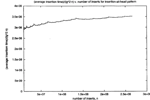
We focus on runtime. Figure 3-3 shows the average time for inserting elements using the insertion-at-head pattern. We don't see the same dips and sharp increases as Figure 3-1 because rebalances occur much more frequently. Figure 3-4 shows the average runtime for the insertion-at-head pattern normalized by dividing by 1g2 n.

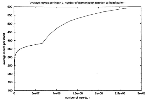
We analyze the number of moves and average rebalancing sum together. Figure 3-6 shows the average number of data moves per insertion for the insertion-at-head pattern. For this pattern, Figure 3-7 shows the average number of data moves per insertion is roughly

E(log2

N). For the insertion-at-head pattern, Figure 3-9 shows the average cost of

rebal-ancing per element. Figure 3-10 shows the average cost of rebalrebal-ancing is roughly E(log2 N).

For all of these graphs, note a sharp change of behavior around n = 108. At n - 108, the

section size doubles from 512 to 1024. The next time the section size is to double is roughly

n = 6 - 10". Given such large intervals between section size doubling, perhaps a smarter

method of resizing the array is needed to achieve more consistent asymptotic behavior. average insertion time v. number of inserts for random insertion pattern

5e-06 4.5e-06 --4e-06 CS3.5e-06 3e-o6 t (D 2e-06 1.5e-06 1e06 -5e-07 -0

5e+07 1 e+08 1.5e+08 2e+08 2.50+08 3e+08 3.5e+08 4e+08 number of Inserts, n

(average insertion time)/(IgA2 n) v. number of inserts for random insertion pattern

5e+07 le+08 1.5e+08 2e+08 2.5e+08 3e+08 3.5e+08 number of inserts, n

time for insertion)/(lg2(number of elements)) with

4e+08

random insertion

average insertion time v. number of inserts for insertion-at-head pattem 3e-05 a, E CA cc 2.5e-05 2e-05 1.5e-05 1 e-05 5e-06 -0 Figure 3-3:

5e+07 1e+08 1.5e+08 2e+08 2.5e+08 3e+08

number of inserts, n

Average time for insertion with insertion-at-head pattern.

7e-09 6e-09 C a .9 t: a, 5e-09 -4e-09 -3e-09 -2e-09 -1e-09 -0 Figure 3-2: pattern. (Average

(average insertion time)/(lg^2 n) v. number of inserts for insertion-at-head pattern

5e+07

time for inse

4e-08 3.5e-08 3e-08 2.5e-08 2e-08 1.5e-08 1e-08 5e-09 0 3e+08 insertion-at-head

average moves per insert v. number of elements for random insertion pattem

CD a) 9 8.5 8 7.5 7 6.5 5.5 5

0 5e+07 1e+08 1.50+08 20+08 2.50+08 30+08 3.5e+08 4e+08

number of inserts, n

Figure 3-5: Average number of data moves with random insertion pattern.

C

ce

01

1 e+08 1.5e+08 2e+08 2.5e+08

number of inserts, n

rtion)/(lg2(number of elements)) with Figure 3-4: (Average

average moves per insert v. number of elements for insertion-at-head pattern 600 550 500 450 400 350 300 250 200 150 100

1.5e+08 2e+08 2.5e+08 30+08

number of inserts, n

data moves with insertion-at-head pattern.

(average moves per insert)/(Ig^2 n) v. number of inserts for insertion-at-head pattern

0 5e+07 1e+08 1.50+08 2e+08 2.50+08 number of Inserts, n

(Average number of data moves)/(1g2(number of elements))

30+08 with insertion-at-E (D 0a EU le+08 0 5e+07

Figure 3-6: Average number of

0.8 0.75 0.7 0.65 C C 0 (U 0 E 0 01 (U e (U 0.55 F Figure 3-7: head pattern. 5 M

average rebalancing sum v. number of elements for random insertion pattern C E 0 0.08 0.07 0.06 0.05 0.04 0.03 0.02 0.01

0 5e+07 1e+08 1.5e+08 2e+08 2.5e+08 3e+08 3.5e+08 4e+08

number of inserts, n

Figure 3-8: Average rebalancing sum with random insertion pattern.

average rebalancing sum v. number of elements for insertion-at-head pattern

-F E CD i; 220 200 180 160 140 120 100 80 60 40 on

0 50+07 18+08 1.5e+08 2e+08 2.5e+08 3e+08

number of inserts, n

Figure 3-9: Average rebalancing sum with insertion-at-head pattern.

(average rebalancing sum)/(IgA2 n) v. number of inserts for insertion-at-head pattern CJ= 0 C .0 T) 0D C" 0.28 0.26 0.24 0.22 0.2 0.18 0.16 0.14 0.12 ni

0 5e+07 1e+08 1.5e+08 2e+08 2.5e+08

number of inserts, n

Figure 3-10: (Average rebalancing sum)/(1g2(number of elements)) with pattern.

3e+08

Chapter 4

Static Cache-Oblivious Binary Tree

Implementation

Chapter 2 described the two data structures that form the COB-Tree, a static cache-oblivious binary tree with a van Emde Boas layout, and a packed memory structure. Chapter 3 provided experimental results. This chapter presents implementation details of a tree with a van Emde Boas layout. Chapter 5 presents implementation details of the packed memory structure.

The tree is represented in memory as an array. The value at location i of the array corresponds to some node of the tree. We need a way of computing the location of the left and right children of node i. One solution is to have the array store pointers, but pointers cost space. Instead, we wish to have an array such that the root of the tree is the first element of the array, and for a given node located at array location i, the locations of the dode's two children are easily found. This chapter provides details.

Consider the breadth-first layout, a simple tree layout. In a breadth-first layout, a binary tree of N nodes is represented as an array. Each element of the array corresponds to a node. The values held in the array are values of nodes. The root node is located at the first position of the array. The locations of the children of node i are 2i and 2i + 1. Thus, the location of children may be implicitly calculated. Implicit calculations of children makes the

breadth-first layout simple to use and conserves space by not allocating pointers for clilldren of nodes. Figure 4-1 shows an example of a binary tree with breadth-first indices, along with van Emde Boas indices.

El K4 26K 29Q

6C 7 1 ( 10 ' t 6 '('D 15( 4 2 27C2 3003

Figure 4-1: van Emde Boas and Breadth First indices on tree of height 5. van Emde Boas

indices are in black letters. Breadth first indices are in white letters. Figure taken from

[7].

We create the same advantages for the van Emde Boas layout by creating an abstraction for the van Emde Boas layout using the breadth-first layout. We maintain an array of values such that the order of nodes is the same as the van Emde Boas layout. However, we provide a function so that the programmer deals with the array as though it has a breadth-first layout. The function converts breadth-first layout indices to van Emde Boas layout indices.

My function, normToBoas, takes O(log log N) word operations. For example, given the tree in Figure 4-1, normToBoas(12) returns 20. Thus, a tree with a van Emde Boas layout will be an array in memory.

Having a function calculate indices from the breadth first layout to the van Emde Boas layout has several advantages. The function makes the creation of a tree with a van Emide Boas layout very simple. To create a tree with N nodes, one allocates an array of size N.

The programmer may program with the ease of using a tree with a breadth-first layout, but gains the locality advantages of using a tree with a van Emde Boas layout. The actual layout of the tree is abstracted away from the user. As far as the programmer is concerned, the system provides a breadth-first tree that runs very efficiently.

a binary search on a tree with a breadth-first layout. The variables, depth and height, are the depth of the current node and height of the tree, respectively. If the value is present, the program returns 1, otherwise, 0. To run the program on a tree of height 5, execute search(tree,1,1,5,value).

int search(int* tree, int node, int depth, int height, int value){ if (depth > height) return 0;

else if (tree[node]==value)return 1;

else if (tree[node]<value)

return search(tree, 2*node, depth+1,height,value);

else if (tree[node]>value)

return search(tree, 2*node+1, depth+1,height,value);

}

Given an efficient normToBoas function, here is the code to do a search on a tree with a van Emde Boas layout.

int search(int* tree, int node, int depth, int height, int value){

int boasNode;

boasNode=normToBoas(node);

if (depth > height) return 0;

else if (tree [boasNode]==value)return 1;

else if (tree[boasNode]<value)

return search(tree, 2*node, depth+1,height,value);

else if (tree[boasNode]>value)

return search(tree, 2*node+1, depth+1,height,value);

}

Note that only two lines of code are added.

The rest of the chapter is organized as follows. Section 4.1 presents the algorithm to convert a node's breadth-first index to the corresponding van Emde Boas index, without

specifying how to evaluate certain intermediate variables. Sections 4.2-4.4 present the algo-rithms to evaluate these variables.

4.1

Algorithm to Convert Breadth-First Index to van

Emde Boas Index

The recursive algorithm to convert a node with breadth-first index n to the corresponding van Emde Boas index is as follows. Given depth d, and height h of node n, we solve for normToBoas(n, d, h). Let the breadth-first layout and the van Emde Boas layout be indexed at 1. For the base case, if h < 3, the van Emde Boas index is identical to the

breadth-first index. Otherwise, let A, B1, B2,..., B be the subtrees recursively laid out in order,

as shown in Figure 4-2. Let h, be the height of A, and h2 be the height of B1,... , B. If

n E A (which only happens if d < hi), recursively call normToBoas(n, d, hj). Otherwise, let n E Bi for some i. Let n' be the breadth-first index of n in B. Let d' be the depth of n in B2. Let x be the total number of nodes in A, B1,... , Bj_1. The final result is x + normToBoas(n', d', h2). Given we can solve for the variables hl, h2, n', d', x in constant

word computations, this algorithm does O(log log N) word computations, where N is the number of nodes in the tree. In the following subsections we present the methods to solve for hl, h2, n', d', and, x using a constant number of word computations.

4.2

Evaluating Heights of Subtrees

We present the algorithm to solve for the height of subtree A, hl, and the height of remaining subtrees, h2. We know h, + h2 = h and h, so we focus our efforts on only evaluating h2. Let

the hyperceil of n be the smallest power of 2 greater than or equal to n. Let the hyperfloor of n to be the largest power of 2 less than or equal to n. Note that if n is a power of 2, then the hyperfloor and hyperceil are equivalent. Otherwise, the hyperceil is twice the hyperfloor.

A B1 B1

B1 _ Bt VN

Figure 4-2: General method of van Emde Boas layout. In memory, the subtrees

A. B1, B2, .. . , B, are recursively laid out in order. Figure taken from [7].

the hyperfloor of h/2.

The implementation for solving the hyperfloor of a, number n is as follows. Let

n

be an unsigned integer. Consider the bit representation of n and of hyperfloor(n). The hyperfloor has only one 1, the highest positioned 1 in the bit representation of n. For example, let n be 25. The bit representation of n would be 00 .. .011001. The hyperfloor, 16, would be 00 ... 010000. We have two variables, va1=1 and temp=n. We alternately right-shift temp

one space (effectively dividing temp by 2) and left-shift val one space (multiplying val by 2) until temp=1. Upon termination, val holds the hyperfloor of n. An example of this execution for n = 25 is in Table 4.1. The code for hyperceil is presented below. The variable

initial values final values

temp 00 .. .011001 00 .. .001100 00 .. .000110 00.. .000011 00 .. .000001

val 00.. .000001 00.. .000010 00.. .000100 00.. .001000 00.. .010000

Table 4.1: Values of temp and val in executing hyperfloor(25).

val stores the hyperfloor. The last line returns the hyperceil, based on the value of val.

inline unsigned int hyperceil-int(unsigned int num) { unsigned int val = 1;

unsigned int temp = num;

temp = temp>>1; val = val<<1;

}

return (val == num) ? val : (val<<1);

}

4.3

Evaluating New Depth and Number of Preceding

Nodes

We show how to evaluate the new depth, d' of the recursive case and the number of nodes in preceding subtrees, x. Given n E Bi for some i, and we have evaluated hl, we know

d' = d - hi. Otherwise, d' = d. We now focus on solving x. Let a be the number of nodes in

subtree A and b be the number of nodes any subtree B1, ... , B. We know x = a + (i - 1)b.

We focus on solving a and b. Let y be the breadth-first index of the root node of B1. We

know y = ₂h1 because of the nature of the breadth-first layout. We also know y is the first

node to be placed in memory immediately after all nodes in subtree A. Thus, a = y - 1.

Similarly, we know b = ₂h2 - 1. To solve for i, we take advantage of the fact we know the

breadth first indices of the roots of B1, ... , B1. We know the root of B1 is 2h 1, the root of

B2 is 2h1 + 1, and so on. The root of B is 2" + i - 1. Thus, solving the breadth first index

of the root of Bi solves the value of i. We know the difference in depth between node n and the root of Bi is d - hl. We know the parent of an arbitrary node, j, is [j/2J. We can evaluate the parent by right-shifting

j

by one bit. Thus, to evaluate the root of Bi, which is

a distance d - (hi + 1) from n, we right-shift n by d - h, - 1 = d' - 1 bits. This solves the

root index of Bi. From this, we can evaluate i.

To illustrate, take a tree of height 7. Therefore, h, = 3 and h2 = 4. The recursive subtrees are A, B1, B2,... B8. Given h, = 3, we know the root of B1 is node 8 of the breadth-first

layout. Suppose n = 46 and d = 6. We know n is located in some subtree Bi. We see d' - 1 = d - hi - 1 =2, a = 23 = 8, and b = 2' = 16. Right-shifting 46 = 000 ... 0101110

two bits gives us the root of Bi to be 000. .0001011 = 11. Therefore, x 7 + (11 - 8) * 15.

Figure 4-3 illustrates the tree.

46

subtree A

<- subtree B4

Figure 4-3: A partial diagram of a tree with height 7 in breadth-first order. The seven

nodes at the top three depths make up subtree A of the van Emde Boas layout. The subtree with root node 11 forms subtree B4 of the van Emde Boas layout.

4.4

Evaluating Breadth-First Index of Recursive Case

Given n E B for some i, the breadth-first index of node n in subtree Bi is n'. We show

how to evaluate n'. We know right-shifting n by d' - 1 bits give us the root of Bi. We want right-shifting n' by d' - 1 bits to give us 1. Thus, the last d' - 1 bits of n and n' are

identical. We wish to change the remaining bits to the integer value 1. For example, take Figure 4-3. Suppose h = 7, n = 46 and d' = 3. We wish to set n' to 6. Let integers be represented by k bits. We know the bit representation of 46 is 000 ... 0101110. We know the bit representation of 6 is 0 ... 0000110. We wish to keep the last two bits, 10, unchanged,

but change the first k - 2 bits from 000 ... 01011 to 000 ... 00001.

1

2

To change the first k - 2 bits to 0000.. .0001 may be done easily. In the bit representation of n, we know the dth bit is a 1 and all higher order bits are 0. Thus, to evaluate n', we need to right-shift bits up to position d to position d'. For example, for n = 46 and d = 6, we need to take all bits from 6 and above and shift them to location d' = 3. This would,

in effect, eliminate bits in [3,6). A simple function, shown below, achieves this goal. This evaluates n'.

inline size.t fixBits(sizet x, unsigned int i, unsigned int

j)

{

unsigned long y = (x>>j)<<i; unsigned long z = x&((l<<i)-l);

return y+z;

Chapter 5

Packed Memory Structure

Implementation

Chapters 2 and 3 presented COB-Trees and their performance results. Chapter 4 presented implementation details of one component of the COB-Tree, the static cache-oblivious binary tree. This chapter presents implementation details of the packed memory structure.

The chapter is organized as follows. Section 5.1 lists several decisions important to making the implementation efficient. Section 5.2 presents detailed descriptions of the implementation of each phase of the insertion algorithm, with the exception of rebalancing. Section 5.3 introduces several possible rebalancing algorithms.

5.1

Data Representation

We present our data representation decisions for the packed memory structure. Below is a list of decisions made to make the packed memory structure efficient.

1. The packed memory structure and binary tree are separately stored as arrays. We

employ memory mapping to store the two arrays consecutively in memory. This allows the data to be used as a single level store.

2. The size of the array T, is a power of 2. The array is divided into sections of size S such that S is the power of 2 arithmetically closest to 1g2

T. Note that (v/-/2) lg2 T <

S < V2 lg2

T, thus S = E(log2

T). As a result, the number of sections, N, is a power

of 2 as well. S, T, and h are all global variables.

3. The relationship between a leaf of the binary tree and its corresponding section is

implicit. Given the breadth-first index of the leaf, we simply need to subtract 2h-1

from the index to evaluate the corresponding section.

4. The binary tree of height h is stored as an array. Note that no information needs to be held at the leaf of a tree. We do not need to access a key because no searching remains. We do not need to store corresponding sections because they may be evalu-ated implicitly. Thus, there is no reason to allocate space for the leaves of the array. Therefore, although we implicitly use a tree of height h with a breadth-first layout, we represent the tree in memory as a tree of height h - 1 with a van Emde Boas layout.

5.2

Insertion

We present implementation details for each part of the insertion algorithm. Suppose we wish to insert i and have found the appropriate section j. The insertion algorithm has several parts. First, the precise location within

j

must be found. Second, threshold must be tested. Then, there are three possible cases. The first case is that the section, j, is within threshold, and the element is inserted. The second cases is

j

is not within threshold, but some portion containing j is. The third case is no ancestor is within threshold and the array needs to be resized. We present issues and solutions for each phase and case.

Finding the Proper Location of i within the Section. The goal is to find the proper location for i as quickly as possible. A poor, yet simple, solution is to perform a linear scan of the section. This strategy works well with small databases, but not with large ones. Although small in comparison to the entire packed memory structure, for large databases, sections

become large enough so that performing a linear scan noticeably slows down performance. Instead, perform a binary search within the section to find the proper location of i. Although tricky to program because the section has empty spaces, a binary search within section j is efficient.

Testing a Section to be within Threshold. When inserting, we do not explicitly test if a section is within threshold, because testing threshold requires scanning the entire section. Just as scanning to find the appropriate location of an element i is too costly, so is scanning to find the density. Instead, an attempt is made to insert i. If an empty space is found, the element is inserted. Otherwise, the density is 1 and the section is not within threshold. We proceed to find a portion to rebalance. Thus, we require the upper bound threshold for a section to be 1.

Insertion within a Section. Given the section, j, is within threshold, we insert i as efficiently as possible. We shift as few elements as possible to insert i. Via a binary search, we find between what two values the element i should be inserted. If empty spaces between the values exist, i is inserted somewhere between the two values. Otherwise, we scan left until we find an empty location, shift all elements up to that location left one space, and insert i. If no empty space exists, we attempt the same thing in the right direction. One of these procedures must work because the section is within threshold.

When inserting into a section, we never need to update the binary tree. When traversing the tree, we traverse down a left branch if and only if the key we wish to insert is strictly less than the key located at the node. Therefore, we never insert a key into a section that is larger than all existing keys in the section. Thus, for this case, the tree never needs to be updated. If we delete the largest element in a section, we choose not to update the tree. Correctness is not affected and we believe the effect on performance is negligible.

Inserting an Element when Rebalancing is Required. We wish to insert the key and

has several issues, along with several possible solutions, all of which are presented in the next section. We focus on updating the search tree. Suppose we have found and rebalanced the proper portion that will contain i. The subtree rooted at the node in the tree representing the rebalanced portion is no longer valid. We must update the subtree representing this portion. This can be done recursively. If the node is a leaf, return the maximum value of the represented section. Every internal node solves for two values from its children, the largest key in each child's portion. Thus, the node returns the value received by the right child, the

largest key in the node's own portion, and stores the value returned by the left child, the largest key in the left child's portion. The code is presented below.

long long int updateTree(node* tree, size-t index, pair* array){

long long int left, right;

if(isLeaf(index)) {

return //maximum value of section represented;

}

else {

left = updateTree(tree, 2*index, array); right = updateTree(tree, 2*index+1, array); tree[boaslocl.val = left;

return right;

5.3

Rebalancing

The problem is as follows. Suppose we have an element, i, we wish to insert. Suppose the section where i is to be inserted, section j, is completely full. The problem is finding the smallest portion containing j that is within threshold and rebalancing that portion as efficiently as possible. We do not address rebalancing and inserting the element concurrently.