Business system improvements through recognition of process variability

(1)

Business System Improvements Through Recognition of Process Variability

by

Michael P. Miller

BS Chemical Engineering, University of Florida, 1988 Submitted to the Sloan School of Management

and the Department of Chemical Engineering in partial fulfillment of the requirements for the degrees of

Master of Science in Management and

Master of Science in Chemical Engineering at the

Massachusetts Institute of Technology June 1997

Signature of Author

Sl an School of MBnagement Department of Chemical Engineering May 15, 1997 Certified by

Stephen C. Graves, Professor MIT Sloan School of Management Certified by

Accepted by

Gregory J. McRae, Bayer Professor Department of Chemical Engineering

Robert E. Cohen, St. Laurent Professor of Chemical Engineering Chairman, Committee on Graduate Students

Larry Abeln, Director of Master's Program Sloan School of Management

JUL 0 1 1991

Science

(2)

(3)

Business System Improvements Through Recognition of Process Variability

by

Michael P. Miller

Submitted to the Sloan School of Management and the Department of Chemical Engineering in partial fulfillment of the requirements for the degrees of

Master of Science in Management and Master of Science in Chemical Engineering

ABSTRACT

Production planning and scheduling systems that do not recognize true process variability will incur significant schedule disruption and require substantial inventories to maintain customer service. When variability is misunderstood or ignored, significant differences will exist between planned and actual utilization. This thesis analyzes the various forms of process variability affecting the supply of usable wide roll from the Commercial Film Flow sensitizing operation at Eastman Kodak Company. It evaluates the existing policies used by this operation to accommodate these sources of variability. Then, through statistical analysis, it provides improved methods for planning and scheduling production and for determining inventory safety stock levels to reduce the impact of these sources of variability. This work shows that by segmenting the sources of process variability into three forms (common cause process, uncommon cause process, and test release), one can design and implement planning, scheduling, and inventory stocking policies specifically designed for each of these forms.

The financial benefits to the Commercial Film Flow Division and Eastman Kodak Company through the implementation thus far of the concepts developed by this thesis have been estimated by Eastman Kodak Company at the following: an approximate $7 million one-time reduction in wide roll inventory, an approximate $2 million annual savings in carrying cost associated with the inventory reduction, and an approximate $200,000 annual savings in planning resources. Additionally, it is believed there are significant financial benefits to Eastman Kodak Company in lowered raw material

inventories due to reduced disruption transmitted upstream from the sensitizing schedule. Thesis Supervisors: Stephen C. Graves, Professor of Management

(4)

(5)

Acknowledgments

I would like to thank the people at Kodak who found time to provide me information, answer my questions, and listen to my findings. Special thanks go to my advisors: Earl Chapman and Bob Rich at Kodak, and Steve Graves and Gregory McRae at MIT for all their support and guidance. My thanks also to the many Kodak people who helped me in my research including Jake Vankouwenberg, Debbie Spratt, Jan Voglesong, Margie Mountain, Laurie Stefanski, Dave Swann, Tom Page and many others too numerous to name. A particular thanks to the Kodak Park LFM alumni (especially Charlie DeWitt, Tao Ye, and Mark Kurz) who made sure I had the resources I needed and that I was "being taken care of."

I am thankful to Tom Braun and Danny Westerfelt for supporting the project and my involvement in it.

I gratefully acknowledges the support and resources made available to him through the MIT Leaders for Manufacturing program, a partnership between MIT and major U.S. manufacturing companies.

Finally, and most importantly, deepest sincere appreciation to my wife Cindy for tolerating all the moves, keeping our lives going, and raising two beautiful children as well.

(6)

(7)

LIST OF FIGURES

Figure 1: Simplified film production process flow 18

Figure 2: Manufacturability by product category 19

Figure 3: Planning and Scheduling of Kodak Commercial Film Manufacturing 20 Figure 4: Sources of variability in fit-for-use sensitized wide roll quantity 24 Figure 5: Schedule loading disparity or "scheduling bow wave" 30

Figure 6: Weekly production hours planned 34

Figure 7: Average of sensitizing machine weekly hours planned vs. number of weeks into the

future (2/96 -9/96) 35

Figure 8: Perfect schedule for sensitizing machine average weekly hours planned vs. number of

weeks into the future 36

Figure 9: Standard deviation of weekly sensitizing hours scheduled by production week vs.

number of weeks into the future 38

Figure 10: Cost Range ($) for schedule changes vs. Number of weeks into the future 39

Figure 11: Depiction of multiple planning cycles in a rolling production schedule 44

Equation 1: MPS Stability Measure 45

Figure 12: Number of schedule changes and stability measure vs. production week 47 Figure 13: Number of schedule changes and stability measure vs. stated reason for change 48 Figure 14: Comparison of period and order-based freeze methods by resulting schedule instability 50 Figure 15: Actual realized footage (%) vs. planned footage for all products sensitized on machine

(1/96 - 11/96) 54

Figure 16: Segmentation of ARF vs. PF data into distinct populations 55 Figure 17: Statistical summary of three population data sets 56 Figure 18: Actual realized footage (%) vs. date for all products sensitized on machine (1/96

-11/96) 58

Figure 19: Number of sensitizing events below 80% ARF vs. month in 1996 59 Figure 20: Frequency distribution of actual realized footage (%) for sensitizing events with

planned footage exceeding 50,000 ft (2/96 -7/96): comparison of actual with normal

expectation 62

Figure 21: Frequency distribution of actual realized footage (%) for sensitizing events with planned footage exceeding 50,000 ft (2/96 -7/96): comparison of actual with normality

expectation excluding incident failures up to ARF 5 68% 63 Figure 22: Two standard deviations around the mean of %ARF vs. PF based on 80% - 120% ARF

on sensitizing machine (1/96 - 9/96) 64

Figure 23: Probability distribution of incident failures (5 80% actual realized footage) on events exceeding 50,000 planned linear feet on the sensitizing machine by number per week (based

on data from 1/96 - 10/96) 66

Figure 24: Cumulative percentage of all sensitizing events sized in hours based on 1997 volume

projections for sensitizing machine 69

Figure 25: Flowchart for calculation method used to derive cumulative distribution of event sizes

in hours 70

Figure 26: Use of headroom when incident failure occurs 72

Figure 27: Headroom action when no incident failure occurs 73

Figure 28: Example table for MAD safety stock calculation 75

Figure 29: Supply safety stock calculations for Graphics codes 78

Figure 30: Confidence intervals +/- (95%) for two standard deviations of a normally distributed

population vs. number of samples 79

Figure 31: Sensitizing bias and 95% confidence intervals by line of business for all products and all events with target footage > 50 KLF and actual realized footage between 80% and 120%

(10)

Figure 32: Confidence that distribution of actual realized footage by line of business is different than that of all events sensitized (with line of business sensitizing biases and events <

50,000 ft removed) for all products running on the sensitizing machine (1/96 -11/96) 83

Figure 33: Sensitized wide roll physical testing tree 88

Figure 34: Distribution of days from sensitizing to release for all rolls sensitized on the machine

(1/2/96 -9/27/96) 89

Figure 35: Cumulative percentage of all rolls released vs. number of days from sensitizing to

release by line of business (1/2/96 -9/27/96) 90

Figure 36: Number of days from sensitizing to release by cumulative percentage of all rolls

released for each line of business (1/2/96 -9/27/96) 91

Figure 37: Number of days from coating to release for 75% and 90% rolls release by line of

business 92

Figure 38: Distribution of days from sensitizing to release for product 3 on the sensitizing

machine (2/96 -9/96) 93

Figure 39: Distribution of days from sensitizing to release for product 4 on the sensitizing

machine (1/96 -10/96) 94

Figure 40: Cumulative distribution of days from sensitizing to release and average finishing rate

for product 3 on the sensitizing machine (1/96 -10/96) 98

Figure 42: Basis for determination of wide roll test variability for safety stocking 100

Figure 43: Inventory vs. time showing number of events frozen by point in the sensitizing cycle 102 Figure 44: Event freeze and timing for stockout protection policy with one frozen event 107

Figure 45: Inventory vs. time for scheduling of n+1 event 109

Figure 46: Average of sensitizing machine weekly machine hours planned vs. number of weeks

(11)

1. Executive Summary

1.1 Thesis Statement

If consistent levels of high quality customer service are to be maintained in the presence of process variability, then there needs to be a focus on inventories, capacity requirements and cycle time. True variability reduction is often slow and tedious because it requires an increased scientific understanding of the products, processes, and their interaction. This work hypothesizes that the planning, scheduling, and safety stocking can be optimized to minimize the impact of process variability on the supply chain.

This thesis will determine and quantify the major sources of process and test variability in the sensitizing operation of Kodak Commercial Film Manufacturing Flow. The thesis then will seek to reduce the impact of the most significant sources of this variability by means of changes in the business system. These changes will consist of improvements in production planning, scheduling, and inventory policies; changes to the information flow; and other means that can be addressed directly. The thesis also will provide a process by which manufacturing can continue to evaluate the sources of variability to ensure that the planning, scheduling and inventory policies accommodate the most current performance data.

1.2 Problem Description

To understand the problems experienced by the Kodak Commercial Film Manufacturing Flow Division (hereafter referred to as the CFM Flow), one must have some

understanding of the system they use for planning and scheduling their manufacturing activities. The CFM Flow uses a classical MRP II (Manufacturing Resources Planning) planning and scheduling process. MRP II is the successor to material requirements planning (MRP), a computer-based tool for scheduling and inventory control developed

(12)

by researchers at IBM.' Hopp and Spearman clearly stated the fundamental insight of MRP:

Dependent demand is different from independent demand. Production to meet dependent demand should be scheduled so as to explicitly recognize its linkage to production to meet independent demand.2

These authors define independent demand as any demand originating outside the system, typically demand for finished products. They define dependent demand as demand for the components making up these finished products. In an MRP system, each finished product (and some intermediate products) has a bill of material (BOM) which defines by quantity and type the components making up that finished product. The production schedule for finished products flows directly from the master production schedule (MPS.) The master production schedule determines net requirements for production by

subtracting current inventory and scheduled receipts from the gross demand.3 The MRP system uses the BOM for each finished product as well as the lead times for materials acquisition and individual manufacturing steps to specify component orders and

manufacturing starts. MRP II is an extension of MRP that takes into account some of the problems of MRP such as schedule infeasibility due to both capacity constraints and stochastic lead times.4

In the case of the CFM Flow, the schedule for sensitizing support with light-sensitive materials (known as sensitizing) comes directly from the master production schedule. The material components required for the operation are determined by bill of material and scheduled by standard lead times. (The reason for making the sensitizing schedule flow directly from the master production schedule instead of an activity scheduled by bill of material will be explained shortly.) This product flow is subject to several sources of

Hopp, Wallace J., and Spearman, Mark L. Factory Physics- Foundations of Manufacturing Management. Irwin Publishing, Chicago (1996), pp. 105.

2 _{ibid., page 106.}

3 ibid., page 108.

(13)

variability including supply, process, test, and demand variability in their common and uncommon cause forms.5 _{Even so, in the interest of minimizing unit manufacturing costs} (UMC), the CFM Flow has sought high utilization (>90%) for the sensitizing process and

scheduled production runs accordingly. Unfortunately, the nature and magnitude of the variability is such that the actual realized capacity of the process has been below the anticipated capacity. This creates frequent schedule changes to ensure the products most in need are being produced first. The CFM Flow has not had a well-devised planning process for dealing with uncommon cause and common cause yield loss as determined at the sensitizing machine or through follow-up testing. The lack of a statistically-based planning process has caused frequent schedule changes in the near-term fixed production schedule (known as the freeze zone), excessive planning and replanning out beyond the near-term fixed production schedule, and appropriate safety stock levels of sensitized wide roll. Individuals within the CFM Flow familiar with the problem and its impact have estimated that a improved planning and scheduling policy with a statistical basis could save from $2 million -$20 million /year depending on the degree of

implementation.

1.3 Thesis Structure

This work accomplishes the following:

* an understanding of the nature of the three forms of process variability (common cause process, uncommon cause process, and test release) that impact availability of sensitized wide roll (Chapter 3.3 and 3.4)

* an understanding of the planning and scheduling phenomena being experienced by the CFM Flow (Chapter 3.1)

s As explained earlier in the thesis, common cause refers to the day-to-day variation of an in-control process whereas uncommon cause refers to variation with a special cause, occurring at a low frequency.

(14)

* a plan for dealing with special cause shortfall in yield of sensitized material. The plan allocates undedicated machine time within the near-term fixed production period of the sensitizing schedule just beyond the expedited lead time for remanufacture of the components necessary to remake the sensitized material in question. (Chapter 4.1)

* a statistically-based, and much simplified determination of safety stocks to accommodate common cause yield variation incurred by all products being sensitized. (Chapter 4.2)

* a statistically-based method for determining and accommodating wide roll test release variation (time and quantity) in safety stock levels. (Chapter 4.3) * a means of combining the various forms of variability to determine

appropriate safety stock levels. (Chapter 4.4)

* a method for combining these forms of variability with demand variability to set wide roll safety stock levels and for freezing larger portions of the wide roll production schedule to allow for reductions in upstream raw material inventory (Chapter 4.4)

1.4 Specific Contributions of this Thesis

The following are actual realized benefits of this work to Eastman Kodak Company: * a reduction in sensitized wide roll safety stocks (implemented: estimated to be

a one-time reduction of $7 million and an annual savings in carrying cost on this inventory of $2 million.)

* a reduction in planning and scheduling resources due to the machine time allocated for rerunning products suffering significant yield loss (implemented: estimated to be an annual savings of $200,000.)

In addition, there is the potential for major reductions in raw material inventory levels resulting from the freedom to enlarge the fixed portion of the sensitizing schedule.

(15)

Finally, since the impact of manufacturing process variability is universal, the

understanding and methodologies presented in this thesis can provide benefit to other manufacturing operations as well.

(16)

(17)

2. Kodak's Existing Manufacturing and Scheduling Process

2.1 Introduction

Kodak's largest film sensitizing facility is Kodak Park in Rochester, NY. Kodak Park's film sensitizing business has two broad product classifications: consumer film and commercial film. There has been an attempt to focus products in each of these two businesses on specific equipment in the interest of matching product complexity with process capability and maximizing overall equipment utilization. Even so, there is some overlap in that any one machine produces a disproportionate mix of products from the two classifications.

Both consumer and commercial film are produced by similar process flow. As Figure 1 shows, chemicals are synthesized at the initial steps of the process. Some of these chemicals are produced internally (SynChem) while others are purchased from the outside. These chemicals are combined with others in various formulas in an emulsion manufacturing step to create emulsion. Support upon which the light-sensitive material will be placed is also being produced in the early stages utilizing either cellulose acetate (acetate) or ESTAR material.

(18)

Figure 1: Simplified film production process flow

Photosensitive emulsion is sensitized onto roll support in the sensitizing step to produce sensitized wide roll. Wide rolls are manufactured in a variety of sizes depending on the specific equipment and product characteristics. These wide rolls are then "finished" or cut and packaged in a multitude of finished product formats.

As mentioned previously, the classical MRP system schedules finished products

independently and sets the requirements for components up the entire process flow based on the finished product schedule. In Kodak Park's case, the wide roll sensitizing

schedule comes directly from the master schedule rather than being treated as a

component of finished product and being set by bill of material and standard lead time. Chemicals, emulsion and roll support are produced according to the wide roll production schedule and sensitized wide roll is finished in a "finish-to-order" or "final assembly schedule" fashion based on actual orders and some amount of in-month production load

(19)

leveling. The reasons for making wide roll sensitizing process the focal point for the master schedule will be discussed in Chapter 2.3.

2.2 Description of the Manufacturing Process for Commercial Film

Commercial film manufacturing differs from other categories primarily in the complexity of the products manufactured and the length of production runs. A good measure for the complexity or manufacturing difficulty of a particular product is the number of individual layers of material that must be applied to the support. As the number of layers increases, the potential for a host of problems increases dramatically as well. These problems include undesirable layer interactions as well as reliable delivery of any one layer. Individuals on the engineering staff of the CFM Flow developed a metric "Increasing degree of difficulty" in an attempt to quantify product manufacturing difficulty. This metric incorporates number of layers as well as other individual user specifications, and contains a factor for product manufacturability. As Figure 2 shows, Commercial film (B*) involves the manufacture of the most complicated products while the manufacture of film in other product sectors (A*) is relatively simple.

45

40

435

32 a

30 *

o

25-

_o

_/~

20

.to e

15-10

_ 5- 2 2

0 .

B K J M H C F G L

Commercial B/W Color Color Commercial

Consumer P' I-%

Line or Dusiness Figure 2: Manufacturability by product category

Differences in the value of this metric correlate with differences in machine efficiency, product yield, unit cost and many other important measures.

(20)

2.3 Current planning and scheduling policies used by the Kodak CFM Flow

A fairly detailed treatment the Kodak MRP II systems architecture is provided by

Kristopher L. Homsi in his thesis Information Flow and Demand Forecasting Issues in a Complex Supply Chain.6 It is necessary here to understand how the wide roll sensitizing operation is planned and scheduled and how this translates to production upstream.

Figure 3 is a graphical depiction of how sensitizing, finishing, and sensitizing components are scheduled as described in Chapter 2.1. As the figure shows, the forecasted demand signal drives the sensitizing production plan which is then

"assimilated" with projected finishing rates and adjusted to meet actual finishing usage.

Wide Roll

Inventory

MRP Signal

MPS Signal

Final Assembly

/

Schedule

Sales Forecast

Figure 3: Planning and Scheduling of Kodak Commercial Film Manufacturing There are three major reasons for having the sensitizing schedule flow directly from the sales forecast through the master production schedule. The most important reason is that

6 Homsi, Kristopher. LFM Masters Thesis: Information Flow and Demand Forecasting Issues in a Complex Supply Chain. MIT Sloan School of Management, MIT Department of Chemical Engineering, (1995), pp. 19-22.

(21)

the number of different items produced by sensitizing is significantly smaller than the number of finished good items. A single sensitized wide roll product can be finished into numerous final formats, consequently master scheduling the finished format would require substantial wide roll product inventories. Driving sensitizing operations purely from actual finishing needs would require larger safety stocks of wide roll or significantly more sensitizing capacity in order to maintain service levels to finishing. Wilson, in his LFM masters thesis Determination of Optimal Safety Stock Levels for Components in an Instant Film Assembly System, demonstrated the following: "For product line demands which are not perfectly correlated, a reduction in inventory stock can be achieved by holding the inventory in a form that 'pools' the product line demands into a single family."7 Statistically, consider finished products A, B, C, and D that each come from a

single wide roll and that are not perfectly correlated in demand. The following is true about the standard deviation (a) of the demand for that wide roll and the a's of each individual finished product: atot < GA + aB + aC + aD.8 Since safety stock inventory is driven directly by a, the same relationship holds true for safety stock inventory.

The second reason is the relative speed and reliability of the sensitizing and finishing operations. Whereas the sensitizing operation requires considerable lead-time (due to component requirements and high utilization) and is somewhat unreliable in actual product yield, finishing is relatively quick and much more reliable. Since reliable

component lead times and relatively unconstrained capacity of component-manufacturing equipment are requirements for a well-functioning MRP system, treating sensitizing as a component supplier and scheduling it by bill of material would cause significant

disruption. Related to this is the fact that sensitizing equipment is much more capital intensive than finishing equipment. Since the component suppliers in an MRP system

'Wilson, John J. LFM Masters Thesis: Determination of Optimal Safety Stock Levels for Components in an Instant Film Assembly System. MIT Sloan School of Management, MIT Department of Chemical Engineering, (1996), page 39.

(22)

need to be less constrained in capacity than the operations they are supporting, it makes financial sense that sensitizing is not scheduled as an MRP component supplier to finishing through the bill of material.

There is a significant difference in the forecast-based/order-based scheduling balance for sensitizing and finishing. Due to its minimal lead-time and higher reliability, finishing has depended less on forecast than sensitizing and therefore been affected less by demand variability. Finishing strives to maintain a final-assembly schedule system which

recognizes the financial benefits of producing from as short a demand horizon as forecast accuracy and internal cost will allow. These financial benefits flow from the

consideration of safety stock inventory due to demand variability and waste resulting from product changeovers.

Within the 18 month OPAL (Operational Planning at the Aggregate Level) horizon, there is a 12 week planning horizon for wide roll requirements which equates to a master production schedule. The aggregate in OPAL refers to monthly sales expectations by product emulsion family and finishing format.9 A planning horizon of 12 weeks is used since this is the period over which a weekly, item level schedule is considered necessary to ensure all required products will be sensitized as scheduled. Outside of this 12 weeks, the system automatically plans and updates monthly production based on forecasts. Inside of this 12 weeks, all planning changes require manual intervention by wide roll planners. Manual intervention is considered necessary due to the need to consider multiple uncertainties that the OPAL system is not designed to incorporate such as the actual rate of wide roll test release. Primarily, wide roll planners compare the updated finishing demand forecast for each individual wide roll product to its existing wide roll inventory level. At the point where the forward weeks of supply drops below a designed minimum level of projected inventory, a wide roll planner will schedule a wide roll sensitizing "event" or production batch. Since these changes are considered outside the

(23)

lead time of the component suppliers, they are believed to cause minimal disruption to production. The appropriateness of this belief will be explored later in Chapter 3.2.

Inside the 12 week planning horizon, the first five weeks (current + four) are considered fixed. When a particular week of planned production passes within this "frozen" zone, changes can no longer be made by wide roll planners "arbitrarily" since they would require action within the average lead times of the component suppliers. Changing the component supply schedule within the manufacturing lead time of the components causes significant disruption and cost due to overtime due to expedited production, excessive waste due to sub-optimal lot sizing, and poor capacity utilization due to inadequate load leveling. If a change is necessary to prevent a wide roll stockout or customer service impact, the wide roll planner will circulate a form requesting a change in the fixed zone which must be signed by the manager of the sensitizing unit, among others.

2.4 Sources of Variability in Fit-for-Use Wide Roll

A number of factors are seen as causes which necessarily precipitate changes to the wide roll sensitizing production schedule. These factors can be divided into the following four

categories: component supply variability, sensitizing process variability, wide roll test variability, and demand forecast variability. Although this thesis focuses on the analysis and treatment of process and test variability, an explanation of each category of variation is helpful in understanding the operation.

A "sawtooth" diagram provides a good frame for describing the macro sources of variability. As depicted in Figure 4 the left-hand vertical side of any individual "tooth" represents a sensitizing event and the target footage for that event. At a constant finishing rate, wide roll inventory represents a specific amount of footage. The right-hand sloped side of the "tooth" represents depletion of the wide roll inventory by the downstream finishing operation. Ideally with no variation in production or usage (and 0 test time,) the new sensitizing event would occur at the exact moment that the available footage reached

(24)

zero. However, the existence of variation requires that some safety stock be maintained to avoid stockouts.

process variability (% actual realized footage from event)

Wide roll

inventory

--. I '-. scheduled coating event rate of consumption by finishing safety stock (inventory I

minimum) _{demand variability:} component supply

variability

:

Time

test release time variability (lead time

to x% conforming) Figure 4: Sources of variability in fit-for-use sensitized wide roll quantity

Two sources of variability were not analyzed in this work: supply and demand variability. Component supply variability refers to uncertainty in the availability of fit-for-use

emulsion and roll support for the sensitizing operation. Although not studied in this thesis, this is a source of change to the sensitizing schedule due to the relatively high utilization of the component manufacturing equipment. Demand forecast variability refers not to variation in demand specifically, but uncertainty in the accurate prediction of fluctuating demand. The sensitizing operation is scheduled based on a finishing forecast and inaccuracies in this forecast require safety stocks for buffering. Of these two sources of variability, demand variability is by far more significant in terms of disruption to the sensitizing schedule.

(25)

The source of variation studied most thoroughly in this thesis is sensitizing process variability. This can take the form of day-to-day common-cause yield variation but can also occur as significant, uncommon-cause yield loss. The latter is the result of what Kodak refers to as an incident failure during a sensitizing event. An incident failure situation refers to an infrequent incident at the sensitizing operation which requires the run to be aborted or significant emulsion and support to be wasted as a result. In either case, the end result is a significant shortfall in footage that cannot be characterized as part of the normal distribution of outcomes.

From the limited analysis conducted by the author into the magnitude and impact of demand variability, it would appear that this source is more disruptive to the sensitizing schedule than process variability. This is in part a result not only of demand's higher standard deviation but the fact that demand can vary both in quantity and time. Process variability manifests primarily in quantity, whereas the start time of an event does not vary as significantly from when it was originally scheduled. Knowing when a sensitizing

event will occur, a wide roll planner can be reasonably confident that some good product will result from the event. Even if there is a shortfall in footage from the event, that which is produced to specification can be used to satisfy demand until an adjustment to the future sensitizing schedule can be made.

Although demand variability causes more disruption to the sensitizing schedule than process variability, Kodak directed the author to focus on process variability. This was due primarily to the fact that most felt there was more opportunity for understanding and improving the response to process variability than for demand variability. Demand variability comes from outside the CFM Flow, and therefore individuals inside the CFM Flow have limited control over it.

With regard to incident failures, the planning system implicitly plans as if these don't occur, even though they occur at a striking frequency. Data to support this supposition

(26)

will be provided in Chapters 3 and 4. Because products are scheduled when they are needed, an incident failure creates an unplanned situation. When an incident failure is

discovered either at the machine or after testing, the planning team must create room in the near-term schedule in order to fit the rescheduled event. Not only is the timing for this typically less than the lead time of the components but it creates a "domino" scheduling effect on other products that must be rescheduled to make way for the new event. These new events many times must occur within the fixed zone of the schedule, discussed in detail in Chapter 3.2. There is definite cost to this practice and it, at the least, keeps the flow from making significant reductions in upstream inventories due to the unreliability of the schedule. The near-term schedule disruption caused by incident failures is similar to that created by non-standard downtime'l (NSDT) on the machine in that each creates an immediate unexpected situation. The usual effect is that the time to produce a certain product is longer than what the safety factors allow. Undedicated capacity in each week's schedule can accommodate a considerable amount of these extended runtimes, but when it is extreme, it can cause one week's schedule to spill into the next week. This then creates the need to reprioritize the scheduling of many events.

In the case of common cause yield variation, there is the temptation to make changes in the plan out beyond the fixed zone as a result of each event's outcome whether in control or not. This practice also limits the extent to which uncertainty passed upstream to raw material suppliers can be dampened by inventory management. Part of the policy proposed by this thesis will address when changes should and should not be made and what safety stock levels are necessary to allow the planning team this confidence.

1o The sensitizing schedule includes some undedicated capacity to allow for standard downtime on the machine such as would be required standard product changeovers and standard quality checks at the beginning of sensitizing events. Non-standard downtime refers to that downtime on the machine which is the result of unexpected occurrences such as significant quality problems or an excessively long product changeover. This non-standard downtime shifts the timing of all subsequent scheduled events and

(27)

Test time and test yield variation (referred to collectively as test variability) are the other sources of variability which have a significant impact on the sensitizing schedule. The product staff tries to qualify just-sensitized wide roll promptly for use by finishing. However, this work must be coordinated with the other priorities of the product staff such as work on new products, improvements on existing products, and trial runs. The

disconnect in the scheduling process is that the sensitizing of wide roll is planned and scheduled but it is fit-for-use wide roll that is needed by finishing. Due to the wide variability in test time and yield, wide roll planners at times feel compelled to reschedule new events for products that have not made it out of testing in a timely fashion. Test variability will be discussed in detail in Chapter 4.3. This thesis will also respond to the need for statistically-based decision tools around when events should be rescheduled and when safety lead time and safety stock should be adjusted to minimize the need for unnecessary rescheduling and unreasonable wide roll inventories.

(28)

(29)

3. General Findings and Analysis

3.1 The schedule loading disparity or "scheduling bow wave"

The term "scheduling bow wave" and the concept it represents were new to the author when he arrived at Kodak for the internship and do not seem to pervade planning and

scheduling culture as a whole. (The scheduling bow wave refers to a machine production schedule with a higher planned utilization in the near future than in the distant future. A further description for and the causes of this phenomena for the Kodak CFM Flow will be given in the remainder of this chapter.) The author found no other reference to this term or phenomenon in any published literature and only one reference in unpublished

company internal literature. An instruction program entitled "Supply Chain Analysis-Managing Uncertainty" created by Greg Kruger of Hewlett Packard (HP), Colorado Springs, CO was the only non-Kodak source describing a "perpetual near-term wave" and "problems associated with running a bow wave."'' Through correspondence with Mr. Kruger, the author learned that HP's bow wave was caused by their

"planning organization intentionally loading their systems with build plans higher than their real expectations for customer demand. The reason planing did this was to create a buffer of extra inventory to handle the

inevitable uncertainty of what demand would be." 12

As mentioned, the author found no reference to the scheduling concept implied by the term bow wave. However, from this point forward, the thesis author will use the term "schedule loading disparity" (or just "disparity" when close in reference to "schedule loading disparity") to describe the bow wave. Although this new term is not fully descriptive of the bow wave phenomena, the reader is asked to associate this term with what the bow wave term represents.

The HP schedule loading disparity differs from that experienced by the Kodak CFM Flow in one major aspect: the HP planning organization uses the disparity intentionally,

" Kruger, Greg. "Supply Chain Analysis- Managing Uncertainty." Hewlett-Packard publication, 7/17/96.

12 Kruger, Greg. Electronic mail sent to author on 3/31/97.

(30)

whereas the Kodak disparity is a result of not understanding and properly accommodating the variability that impacts the sensitizing operation. This will be explained in further detail in Chapter 3.1. However, whether it exists intentionally or unintentionally, a schedule loading disparity causes problems to the organization. In his instruction program, Mr. Kruger lists distrust between planning & procurement and suboptimal inventory levels as the most significant problems created by their schedule loading disparity. They have realized the inadequacy of this policy and have moved to a

statistically-based scheduling policy, similar to what is being used by Kodak CFM Flow, and what this thesis intends to improve.

Figure 5 provides a qualitative representation of Kodak's schedule loading disparity. The shape of the curve implies the continual heavy front loading in a schedule which

decreases over future time.

Planned

Loading

Now

Future

Time

Figure 5: Schedule loading disparity or "scheduling bow wave"

For the purposes here, the author will only deal with the schedule loading disparity as it relates to manufacturing planning and scheduling, but the concepts are transferable to any set of planned and scheduled activities.

(31)

The fundamental root cause for a schedule loading disparity as described is the difference between what an entity predicts it will accomplish and how long it will take, and, what it actually does accomplish and how long it actually does take. This description is at the heart of the need to understand the true performance variability and bias in any plan or

schedule. The projected plan determines resource allocation, short-term capital decisions, maintenance schedules, and a host of other activities. Disrupting these after an intention or commitment to execute is costly and frankly demotivating to those involved. Future plans should reflect past performance accurately and should not be an unrealistic representation of anticipated learning or assume variability that is lower than what actually exists. An understanding of the nature of the difference between anticipated and demonstrated performance is critical to making plans that are both feasible and cost-effective.13 _{One study of rationality in expected performance for production stated:}

The management of the firms have both preference for and are personally committed to a higher production...In their attempt to predict the future

production, the management will assume normal operating conditions and does not take account of unusual conditions such as machine breakdown, delivery delays...which lower future production...The "over optimism" bias is furthermore hypothesized to increase with the uncertainty of production measured by its

variance.14

The last sentence above seems appropriate to the CFM Flow given the relatively high frequency of incident failures and the significant common cause variability. In classical capacity planning, one does not make allowances for "all or nothing" yield loss and usually underestimates the inherent variability. As production continues, it seems natural that expectations for successful production will be overly optimistic and result in a bow

wave.

'3 An example of the lack of understanding by an organization experiencing a scheduling bow wave is the tendency to conclude that although the plan may seem infeasible over the next x number of time periods, once the organization gets beyond this, the plan should be feasible. Without fixing the root causes of the bow wave though, this improvement in schedule feasibility will not occur.

14 Madsen, Jakob Brochner. "Test of rationality versus an 'over optimist' bias." Journal of Economic

(32)

3.1.1 Root causes of the schedule loading disparity

In a discussion early in the internship with a material supply manager about the drivers of the schedule loading disparity, the manager mentioned four root causes:

1. Product variation- occurs when at least one of the components, usually an emulsion layer, is not performing well upon sensitizing. This problem is discovered through testing during the initial stages of the production run and usually results in an aborted run (i.e. little or no yield.)

2. Process variation- this can take the form of minor variation as in subtle variations in pump speed or significant variation as in air entrainment in a liquid delivery system depositing bubbles onto the wide roll. The latter most likely results in an unplanned stop of the sensitizing machine to allow liquid lines to be purged of air. The act of shutting down and starting up the machine consumes a fair amount of emulsion and support which would otherwise be transformed into sensitized wide roll.

3. Wide rolls found by testing to be unusable- this quantity, referred to as shrink, is wide roll that was not scrapped at the sensitizing machine but has failed post-production qualification.

4. Timing of disposition of wide roll, the quality of which is uncertain- this is variation in the testing time for determining the ultimate disposition of sensitized wide roll.

This thesis combines product and process variation since their existence isn't discovered until sensitizing begins and since they have the same effect of causing a shortfall in yield for a sensitizing event. Wide rolls found by testing to be unusable and timing of wide roll disposition have also been combined into test variation. The difficulties of dealing with uncertainty in both quantity and time will be addressed later in the thesis. Although not mentioned during the interview with the supply manager, there are also other causes of the schedule loading disparity:

(33)

5. Demand variability- as mentioned earlier, this is essentially forecast accuracy. It must be included as a root cause since it can result in unanticipated volume being placed in the near-term sensitizing schedule.

6. Sensitizing bias- this represents the difference between the quantity of wide roll that is intended to result from a certain quantity of components with no variation and the quantity of wide roll that actually does result. If the CFM Flow runs a continual negative bias, then it will forever be needing to make up the difference between the target footage and the actual long-term mean

footage.

7. Demand bias- analogous to sensitizing bias in that it represents the long-run average difference between the predicted demand and the actual demand. A continual negative demand bias will also require near-term "overdrive."

3.1.2 The schedule loading disparity confirmed with data

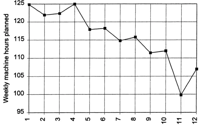
Although sensitizing capacity plans developed by the capacity planner appeared to show a schedule loading disparity over the future 12 weeks, the author sought to determine the extent of its presence in weekly schedules. A technique developed by the thesis author used the weekly twelve-week sensitizing production schedules from 2/28/96 to 10/10/96 as inputs. Week 20 through week 35 had complete data for each of the twelve weeks, while the twelve weeks immediately prior to week 20 and the six weeks immediately after week 35 had partial data. Figure 6 is a subset of the entire data set showing how the data was handled.

(34)

Week of Date of

Schedule Schedule Week in future for which production is scheduled

Creation Creation 20 21 22 23 24 25 26 27 28 29 30 31

Each value represents the planned weekly

9 2/28 74" machine hours created on the day shown in

10 3/5 51 112 left-hand column for the production weeks

11 3/14 129 113 114 shown along the row heading above 12 3/21 100 91 114 123 13 3/28 84 101 113 103 73 14 4/4 96 101 116 124 99 104 15 4/11 117 116 113 142 125 107 107 16 4/18 113 107 116 151 145 89 133 67 17 4/25 113 100 115 149 146 89 125 71 110 18 5/2 118 140 119 157 147 88 137 70 134 78 19 5/9 145 95 119 124 143 88 135 71 137 99 96 20 5/16 145 102 118 122 147 89 134 73 134 126 82 117

Figure 6: Weekly production hours planned

For example, at the start of production week 20 (the week of 5/16), there was an estimate for each of the twelve future production weeks including week 20 (outlined row.) Also in each of the previous eleven weeks there was an estimate of the production requirements for production week 20 (outlined column.) Taking the average of upper-left to lower-right diagonal across the entire set of twelve-week data yields average planned loading by week in the future. For example, for the data set shown in Figure 6, the mean of the values making up the top diagonal (74, 112, 114, 123, 73, 104, 107, 67, 110, 78, 96, 117) yields the mean planned loading for week 12 of the schedule. The plot of the mean planned loading for each of the twelve weeks scheduled in shown as Figure 7.

(35)

*o r 4) C e -a o (I_L. 0

E

a)

4)

125

120

115

110

105

100

95 I

I

-" M V') LO~ ) D N* C00 0 0

(-Number of weeks into the future

Figure 7: Average of sensitizing machine weekly hours planned vs. number of weeks into the future (2/96 -9/96)

(36)

I cf C\ ) 4 LO C o - cO ) 0

T1_

Number of weeks into the future

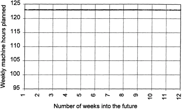
Figure 8: Perfect schedule for sensitizing machine average weekly hours number of weeks into the future

planned vs.

Here the schedule appears as a horizontal line between 120 and 125 machine hours planned per week. This is perfect due to the lack of a schedule loading disparity between the near-term and the long-term. In the perfect case, planners have made necessary and sufficient accommodation for all sources of variability in their estimates for downtime, event duration, and overtime. Knowing that their assessment of actual future

requirements is correct, the organization can make a low-cost allocation of resources significantly ahead of when these resources will be needed. The thesis author placed the line at the level of 123 hours since this is the mean of the hours planned for weeks one through four in Figure 7, the mostly likely representation of the true hours spent on the machine.

Returning to Figure 7, one sees a progression in weekly machine hours planned from about 100 - 105 in week 12 to roughly 120 - 125 in week 1. So this would indicate that over the period this data represents, each production week was increased on average almost a full day of production as it moved across the 12 week horizon. To further

125

120

115

110

105

100

95

c) me CU C') L-0 a) C -c_U to

E

a) a) - - m~

I

C\

(37)

substantiate the existence of the bow wave, the author calculated that approximately 75%

of the individual production weeks had negative slopes in hours/week when considered from week 1 to week 12 of the schedule.

The increase in the average weekly hours planned from 11 to 12 weeks in the future seems not to agree with what is actually occurring. If one looks at the actual data used to generate the curve, removing a 188 hour 12th week projection for week 21 reduces the planned hours estimate for week 12 from 107 to 103. This seems reasonable since there

are only 168 hours in the calendar week. Removing a 146 hour 12th week projection for week 24 reduces the planned hours estimate for week 12 further from 103 to 101. It is not uncommon for planners to designate excessive and unreasonable production in the far

end of the schedule if for no other reason than to tag the suspected need for sensitizing events on particular products. The planners' intend to make the timing more reasonable as the actual production date approaches. Although these unreasonable production plans may be outside the lead time of the component suppliers, it is unacceptable in that it makes resource and capacity allocation decisions suboptimal.

Further evidence of this practice of making an unreasonable schedule in the far weeks of the 12 week sensitizing schedule is provided by Figure 9. Here the standard deviation of planned machine hours is shown by number of weeks in the future. Each data point is the standard deviation of the set of differences between the planned production of the future week indicated and the production for that week as seen one week earlier.

(38)

4 5 6

Number of weeks

7 8

into the future

Figure 9: Standard deviation of weekly sensitizing hours scheduled by week vs. number of weeks into the future

production

For example, from Figure 6, one sees that for production week 20, the difference between the 12 weeks out and 11 weeks out schedule is 23 machine hours (74 -51.) Taking the standard deviation of set of 12 - 11 week differences for all production weeks yields a value of 29, shown for week 11 in Figure 9.

Three characteristics of this plot are noteworthy.'5 _{First, there is significant variation (as} defined in the previous paragraph) out beyond nine weeks in the future. This reinforces the earlier suggestion that unreasonable production is planned frequently at the outer limit of the 12 week planning horizon, and corrected in later weeks. Second, there is a local maximum in the standard deviation at a point five weeks into the future, the outer limit of the fixed zone. This indicates a spike in planning activity at that point as planners

attempt to resolve final scheduling problems before the schedule is fixed and they must

" Note that the author did not perform analysis on this data to determine which of these points were statistically different. >% 0 CD -Y ~Ta) 4- .Ce C o o r, 0) "0 ,. I1) 1 2 3 9 10

(39)

leave it as designed. (The schedule is fixed at this point so as to minimize the scheduling disruption to emulsion and roll support suppliers. The scheduling and production lead time of these suppliers is roughly five weeks, so changes to the sensitizing schedule

would cause changes in activities already set in motion. The fixed zone will be explained in further detail in Chapter 3.2.) Third, the standard deviation continues to decrease as one moves from the point five weeks out towards the production week one week in the future. This indicates that even within the fixed zone, some changes are necessary.

However, there is recognition of the increase in cost as those changes are made closer and closer to the actual production date as estimated by financial analysts within the CFM Flow and shown in Figure 10.

Cost range ($)

10,000's

1,000's 100's _?

Less than One One to Three Three to Five Beyond Five Number of weeks into the future

Figure 10: Cost Range ($) for schedule changes vs. Number of weeks into the future

These are costs within the CFM Flow and include such requirements as simple replanning for changes at outer limit of the fixed zone to expediting new emulsion batches for

changes one to two weeks before the scheduled sensitizing date. The cost range is uncertain for changes beyond five weeks in the future since this would impact suppliers to emulsion and roll support. Reducing the schedule changes that impact raw material

(40)

Reducing the number of requirement changes affecting suppliers by enlarging the sensitizing fixed zone will be discussed further in Chapter 3.2.

When initially confronted with the schedule loading disparity, the thesis author was intrigued but uncertain as to the reason for deep concern. As one supply manager roughly stated, the capacity and inventory planners know they have to do a lot of replanning and additional loading of the near-term schedule, but they still manage to get the products manufactured and meet the customer requirements. However, there are several concerns with adopting this sense of security. The most critical of these is the degree to which overtime on weekends was used to complete production scheduled for the five-day week. As a planned production date approaches the real date, rework and incremental volume are added to the schedule. Provided this extra production did not require more time than was available with weekends and some lighter production weeks, products would be assured of making it through the process at a reliable rate. One must remember that the performance of the sensitizing machine is a distribution such that scheduled production is completed some weeks and runs over in other weeks. Provided there is available

capacity, the probability of successfully completing any scheduled production run within for instance one month from the initial production date is very high. As the available capacity is reduced, the probability of successful completion within a particular timeframe drops and the timeframe necessary to ensure successful completion of

scheduled production increases. A concern with this is that the sensitizing machine went from five-day to seven-day schedule in late 1996 with the intention of adding more volume to the schedule. If adequate weighting is not given to demonstrated performance in assessing future production capabilities, then customer service could suffer due to the

loss of unscheduled weekend time for work overflow.

Another flaw with the confidence in demonstrated schedule completion at some aggregated timeframe is the continued push for reduced cycle time and unit cost in production. Reduced cycle time will require reducing the inventory that serves to

dampen the impact of unsuccessful sensitizing on the finishing operation. It will be less 40

(41)

and less allowable to push some products back to provide machine time to rerun products that suffered low yield. Cost reduction initiatives will continue to make "excess"

capacity unattractive, thus greatly eliminating discretionary machine time for rework.

The leaders of the CFM Flow realize that the planning and scheduling methods currently employed are costly and have been taking steps to improve these methods. One step taken has been simply to reduce the resources dedicated to scheduling sensitizing. The

CFM Flow enacted this change in 1996, independent of the work of this thesis, and found there was no discernible impact to customer service, inventory, or unit cost. This result emphasizes the point that many of the schedule changes being made had added no value. Another step being taken is the addition of emulsion capacity which when in place will reduce emulsion lead-time and the impact of emulsion supply variability on the

sensitizing schedule. Other steps are being taken to make sensitizing data more accessible and manageable so that performance in capacity planning and product scheduling can be tracked more easily and policy adjustments made as necessary. Another very significant change undertaken by the CFM Flow reflects their

understanding of the desirability of a flat utilization schedule. In late 1996, the capacity manager made significant adjustments to the sensitizing capacity plan to provide

undedicated capacity as necessary to meet wide roll requirements with less schedule changes. The impact of these adjustments on schedule loading disparity will be shown in Chapter 4.4.

3.2 Master production schedule stability

3.2.1 Measurement of master production schedule stability in the CFM Flow

It might not be evident why an overly optimistic expectation would lead to a schedule loading disparity. A stable loading disparity (one that does not grow in size indefinitely) requires there to be some undedicated capacity on the operation being scheduled. The period studied by the author did in fact have this capacity in the form of

(42)

initially-unscheduled weekends. As initially-initially-unscheduled weekends "approached" the present, there was increasing likelihood that they would be needed for production in order to maintain customer service. At the point where this capacity was consumed in producing to meet new demand or remaking low-yield product, a "domino effect" of shuffling production began. Prioritization had to be made across the multiple products sharing the machine to determine the sequence of running that minimized cost and jeopardy of stockout. When an unforeseen addition had to be made to the near-term schedule and there was no remaining capacity, machine time had to be created by shifting out other scheduled products. These could not be placed simply on the end of the schedule and therefore, in many cases, needed to take the place of other scheduled products. When capacity was highly utilized, these perturbations rippled across products and across time to a point that the root causes of subsequent schedule changes were not easily traceable.

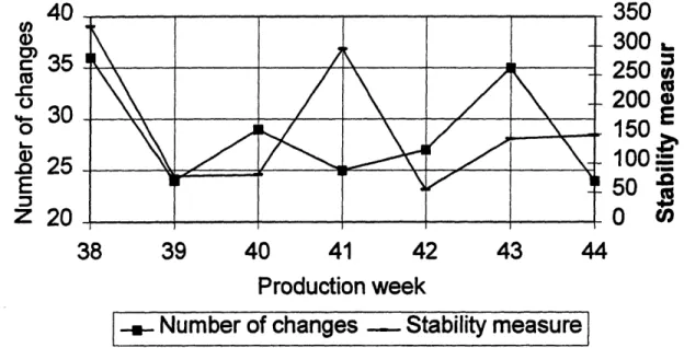
Although the continual rescheduling of schedules was considered by most involved to be suboptimal, changing this practice lacked strong support. This seemed due primarily to poor understanding of the relative impact of the various forms of variability and the costs of rescheduling. It became evident to the author early in the bow wave study that a "schedule disruption metric" would be very valuable in showing which schedule changes were most disruptive and in verifying that process variability was a significant driver of change.

The simplest disruption metric one might create is the pure number of master production schedule (MPS) changes per week. Building on this, one might include the size of the change in quantity of material or machine time affected, whether the product is being shifted in or out in time, and how far in the future the change is occurring. In regards to when the change is occurring, a factor which reflects changes within its cumulative lead time (CLT) freeze zone (identical to fixed zone, defined earlier) different than changes

outside this freeze zone would aid in its accuracy. It would also be helpful to include a measure of overall machine utilization associated with the change since this largely will determine the magnitude of the resulting "domino effect." This need may not be that

(43)

great though since one would expect a significant shift into a highly utilized week to force other changes which would also be recorded. Although one can see easily the directional impact of these various change characteristics, arriving at magnitudes which reflect the overall disruption of the change is much more difficult.

The author searched literature on schedule disruption and found only one reference to a quantitative measure of disruption. Sridharan, Berry, and Udayabhanu 16 developed a measure for schedule instability in the interest of comparing three important decision variables for MPS management in a rolling-horizon framework: the MPS freeze method, the MPS freeze fraction, and the MPS planning horizon length.

Their equation takes into account the following three variables: the number of weeks into the future that the change is occurring, the size of the change (how many units are being added or subtracted), and a weighting factor "that applies decreasing weights to schedule changes in periods of increasing distance in the future."

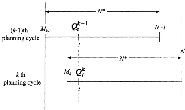
Although Sridharan, Berry, and Udayabhanu do not supply a derivation with their paper, the thesis author will create a derivation adapted to the CFM Flow planning system, using Figure 11 as an aid.

'6 Sridharan, V., Berry, W.L., & Udayabhanu, V. "Measuring master production schedule stability under rolling planning horizons." Decision Sciences, 19, no. 1 (1988): 147-166.

(44)

(k-l)th

Mk-

~

Nt-planning cycle

t

N

N*

kth

4Qt

planning cycle

t

Figure 11: Depiction of multiple planning cycles in a rolling production schedule

The end result should be a relationship that quantifies system disruption created by changes to the production schedule. One can define a production schedule change simply as any alteration in quantity or timing in any period of a previously-established schedule. The Flow uses a planning cycle frequency of once per week and a master production schedule length N* = 12 weeks. The variable k will designate the specific planning cycle in question, and Mk the first period of planning cycle k. The variable t will be defined as the specific time period of the quantity change in question such that a quantity change x weeks from the current week will be designated as occurring in time period t = x. Let Q

be the quantity of a specific product scheduled to be run in time period t and planning cycle k. A weighting parameter a (0 < a < 1) will be used in combination with the quantity t -Mk to weight quantity changes in the near future more heavily than quantity

changes in the distant future. Using the quantity t -Mk as an exponent on a such that it will have a nonlinear effect. (A linear relationship would make schedule changes x/2 weeks in the future twice as disruptive as changes x weeks in the future. In reality,

Business system improvements through recognition of process variability

JUL 0 1 1991

Science

TABLE OF CONTENTS

LIST OF FIGURES

1.

Executive Summary

1.1

Thesis Statement

2. Kodak's Existing Manufacturing and Scheduling Process

45

40

435

32

a

30

*

25-

o

/~

20

15-10

0

.

Wide Roll

Inventory

MRP Signal

MPS Signal

Final Assembly

/

Schedule

Sales Forecast

Wide roll

inventory

:

Time

3. General Findings and Analysis

Planned

Loading

Now

Future

Time

E

a)

125

120

115

110

105

100

95

I

I

I

(-Number of weeks into the future

Number of weeks into the future

125

120

115

110

105

100

95

E

I

I

(k-l)th

~

Nt-planning cycle

N

kth

4Qt

planning cycle

_o

_/~