Capture and control of excitations

(1)

Capture and Control of Excitations

by

Timothy S. Sinclair

B.S. Chemistry

California Institute of Technology, 2015

Submitted to the Department of Chemistry

In partial fulfillment of the requirements for the degree of Doctor of Philosophy

at the

MASSACHUSETTS INSTITUTE OF TECHNOLOGY February 2021

Signature of Author: ____________________________________________________________ Department of Chemistry October 13, 2020

Certified by: __________________________________________________________________ Moungi G. Bawendi Lester Wolfe Professor of Chemistry Thesis Supervisor

Accepted by: _________________________________________________________________ Adam Willard Associate Professor of Chemistry Chair, Department Committee on Graduate Students

(2)

(3)

This doctoral thesis has been examined by a Committee of the Department of Chemistry as follows:

Professor Gabriela S. Schlau-Cohen………..……….... Cabot Career Development Associate Professor

Thesis Committee Chair

Professor Moungi G. Bawendi……… Lester Wolfe Professor of Chemistry

Thesis Supervisor

Professor Troy Van Voorhis……….. Haslam and Dewey Professor of Chemistry

(4)

(5)

5

Capture and Control of Excitations

by

Timothy Sinclair

Submitted to the Department of Chemistry

in partial fulfillment of the requirements for the degree of Doctor of Philosophy in Chemistry,

February, 2021. Abstract

Fundamental understanding of the capture and control of excitations, including photons and excitons, in optoelectronic devices is important to optimizing their performance. Devices such as luminescent solar concentrators and signal concentrators that increase the efficiency of solar energy production and the speed of point-to-point communication, respectively, will be crucial for maximizing the sustainability and connectedness of the world going forward. Behind the workings of these devices are micro-scale interactions of excitations with the device materials that must be carefully modeled and well understood.

In this thesis, I model the performance of both luminescent solar concentrators and signal concentrators using the Monte Carlo method to predict the efficiency from the average results of many trials of quantum behavior. For each of these devices, I propose a path to improved performance. For luminescent solar concentrators, this is the use of tandem fluorophores. In this approach, the addition of a second fluorophore material increases the amount of sunlight that can be absorbed without interfering with the efficiency at which the first fluorophore collects solar photons. For signal concentrators, this is a mutli-aggregate fluorophore with <100 ps fluorescence lifetime that does not re-absorb its own emission because of the introduction of an artificial Stokes’ shift.

In addition, in this thesis I model the photophysical properties of the C8S3 J-aggregate to understand two of its properties: the long exciton migration it exhibits, and its ability to be

irreversibly photobrightened and reversibly photodarkened under continuous illumination. I show the exciton migration distance is due to strong nearest-neighbor coupling along a helical

direction that is aligned close to the axis of the aggregate tube, while the photobrightening and photodarkening behaviors are due to changes in two different types of disorder.

Thesis Supervisor: Moungi G. Bawendi Title: Lester Wolfe Professor of Chemistry

(6)

6

Acknowledgments

Even though this thesis is attributed to a single author, I would never have been able to write it or even do the work it represents without the support of my family, friends, co-workers, and mentors.

When I joined Moungi Bawendi’s lab five years ago, the J-aggregates that captured my interest represented a small subsection of the group’s work, and my ardor for a theoretical approach to their study was not necessarily in Moungi’s wheelhouse as an advisor. I cannot overstate my thanks to Moungi for his constant support and for giving me independence in what work I performed in his lab as I traced a path that ended up crossing with device studies more familiar to the lab as a whole.

Of course, my path would have been a lot more difficult if I did not have great mentors to help me begin my journey, including Justin Caram, Chern Chuang, and Doran Bennett. I am also very grateful for the other members of the group who did work on J-aggregates including Francesca Freyria, Megan Klein, and Ulugbek Barotov. In addition, I want to thank every other member of the Bawendi Lab who I overlapped with, especially the cohort of students who entered the lab at the same time I did, Nicole Moody, Cole Perkinson, and Jason Yoo. Finally, I want to acknowledge all the support of my friends and family, who always warmly welcomed me when I returned home from the other side of the country after I moved even further away from home for grad school than I did for undergrad.

(7)

7

Chapter 0. Introduction

Many of today’s technologies relates to one of two things: converting energy from one form to another, and transmitting a signal over great distances. From the original steam engine, to the coal-fired power plant that powered the Industrial Revolution, to the solar farms that will one day allow humans to ditch fossil fuels, transformation of energy from one form is a fundamental way we control our world. Similarly, every generation going back 150 years has seen our society revolutionized by a means of signal transmission over great distances, from telegraph, to telephone, to radio, to television, to the Internet. Since its discovery, electricity has been both the most interconvertible form of energy and the easiest way to transmit a signal in condensed media. Electrons, however, are not the only particles that can carry energy or information. These particles include charge carriers, such as electrons or holes, photons, and excitons. Holes exist in semiconductors when an electron is excited from the conduction band to the valence band, and the vacated state in the conduction band behaves like the opposite of an electron. Excitons are delocalized excited states made up of a bound electron-hole pair. This thesis examines from a theoretical perspective how control of excitations in

condensed media can lead to new and improved technological applications. Modeling of fundamental properties of excitations in materials and devices elucidates the behavior of excitations in these materials, as well as device performance and optimization.

The first chapter covers simulations of the efficiency of luminescent solar concentrators, a type of photonic device that increases the amount of sunlight a solar cell absorbs. A Monte Carlo method models the behavior of photons within the device waveguide, including impinging solar radiation and light re-emitted within the device. The results of this model closely match experimental results for the efficiency of a thin-film

concentrator. The model predicts that a tandem concentrator with an additional dye layer to absorb redder wavelengths of light has increased efficiency of photon collection. The second chapter covers the understanding of excitonic properties of J-aggregates, a class of supramolecular structures with unique spectral properties including red-shifted absorption and emission spectra relative to the individual molecules. This chapter

(9)

9

develops a model of J-aggregates that explains both long-distance exciton migration and an unusual photobrightening/photodarkening behavior. An exciton hopping model that treats the aggregate as 1-dimensional predicts the >1 micron excition migration observed in exciton-exciton annihilation measurements. Inclusion of connectivity

disorder between the molecules of the aggregate predicts the change in spectra during photodarkening.

Finally, the third chapter covers devices for free-space optical communication, which combine aspects of luminescent solar concentrators and J-aggregates in order to transmit free-space signals at high bitrates. J-aggregates have a fluorescent lifetime much shorter than the quantum dot fluorophores used in luminescent solar

concentrators but need to have an engineered Stokes’ shift in order for their use in signal concentrators for free-space optical communication. Monte Carlo simulations of these devices yield various strategies toward developing devices that can achieve a benchmark 5 Gbps with sufficient efficiency and gain.

(10)

10

Chapter 1. Luminescent Solar Concentrators

1.1 Introduction to Luminescent Solar Concentrators

Luminescent solar concentrators (LSCs) are devices that concentrate solar flux from a larger area to a smaller one.1_{LSCs are frequently coupled to solar cells, and are used}

to increase the amount of solar radiation directed at the coupled solar cell, without increasing the area of the solar cell itself. This can be a cost-saving measure because of the relative low energetic cost of producing an LSC compared to a silicon solar cell that requires high-temperature processing to achieve a high degree of crystallinity and high efficiency.2_{In addition, LSCs may be designed to only concentrate the light}

capable of exciting the solar cell. Such a device would have the advantage over a traditional solar cell of fully transmitting the low-energy light for use in lighting, heating, or upconversion for photovoltaic generation in a subsequent module3,4_{. The general}

design of an LSC consists of two parts: a waveguide, or material of high refractive index in which solar radiation is trapped, and a fluorphore5_{, a flurorescent material that}

absorbs and re-emits the light in such a way to be captured by the solar cell on the edges of the device. The two most basic LSC designs consist of a rectangular waveguide made of a transparent polymer either with the fluorphore uniformly

throughout it, as in an integrated LSC, or with a layer of the fluorphore on the top face of the device, as in a thin-film LSC. There are many possible geometries and design

architectures for LSCs incorporating design elements such as anti-reflective coatings or distributed Bragg reflectors to act as a “one-way mirror” of sorts to better trap

fluorescent radiation, but these are the two most basic designs.6_{For an LSC, the most}

important figure of merit is the overall gain (G). This represents the factor of

magnification of the solar flux experienced by the solar cells on its edge. The overall gain is equal to the geometric gain – GG, the ratio of the area of the LSC impinged by solar radiation to the area of the solar cells – multiplied by the efficiency, or the fraction of impinging solar photons rerouted by the fluorophore and absorbed by the solar cell.

(11)

11 𝐺 = 𝐺𝐺 ∗ 𝑒𝑓𝑓.

Figure 1. An LSC. The geometric gain is the ratio of the top face, in gray, to the area of the sides, in orange. For this LSC, the geometric gain is 2.

In an ideal LSC, the 𝐺𝐺 ≫ 1 and 𝑒𝑓𝑓 ≈ 1. This results in a device that with a high gain. However, several loss mechanisms within the device can cause the efficiency to be much lower than 1. Furthermore, increasing the geometric gain can further reduce the efficiency. Therefore, it is important to understand the loss mechanisms within an LSC not only to optimize the overall efficiency of solar photon capture, but to discover the optimal tradeoff between geometric gain and efficiency in order to have the highest overall gain possible. Besides studying LSCs by building them and comparing their effectiveness to one another, one powerful way of optimizing this system is to model the detailed photophysics of LSC devices to understand what makes a successful LSC.

(12)

12

1.2 Loss Mechanisms in Luminescent Solar Concentrators

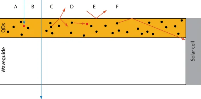
Figure 2. Loss mechanisms and photon capture in a thin-film LSC. A) Loss due to lack of re-emission. B) Transmission loss. C) Escape cone loss vs. internal reflection. D) Re-absorption. E) Reflection loss. F) Photon capture by the solar cell.

The main loss mechanisms in LSCs are reflection, scattering, transmission, lack of re-emission, and escape cone losses, shown in figure 2 above.7_{When a light wave passes}

through an interface with materials of different indices of refraction of either side, a certain fraction of that light will reflect off the interface and a certain fraction transmits through the interface. In the wave picture of light, we describe this as the initial wave of light creating two waves with the same frequency as before but different wavelengths, directions of propagation, and amplitude.8_{The total power transmitted by the two waves}

is the same as in the original wave, conserving energy. In the photon picture of light, we describe this as every photon having a chance to take one of two paths: the reflection path, or the transmission path. The ratio of probabilities of taking each path is the exact same as the ratio of power transmitted in the two waves in the wave picture. When the direction of initial light propagation is normal to the interface, the probabilities of

reflection and transmission of non-polarized light are 𝑅 = |𝑛1− 𝑛2

𝑛₁+ 𝑛₂|

2

(13)

13 𝑇 = 1 − 𝑅.

In a typical LSC, the waveguide polymer has an index of refraction of roughly 1.4-1.5.8,9

The index of refraction of air is 1.00029 at standard temperature and pressure.

Therefore, in a typical LSC, if we assume that the sun is at infinity, we expect reflection losses of roughly 3-4%. Realistically, at least some solar radiation is not going to come directly from the sun perpendicular to the air-waveguide interface, but be scattered by the atmosphere and enter the LSC from an oblique angle.10_{Because of this, real-life}

reflection losses may take into account some portion of the light at normal incidence and some at a distribution at varying angles.

The transmission and lack of re-emission losses are properties of the fluorophore. A fluorophore is a material that displays fluorescence – it absorbs a photon of light, exciting the fluorophore, and then soon afterward relaxes. This relaxation may be radiative, resulting in re-emission of a photon at a lower wavelength in a random direction, or it may be non-radiative, in which the difference in energy between the fluorophore excited state and ground state dissipates as heat.

(14)

14

Figure 3. Energy diagram showing a fluorophore as a two-level system. From left to right: absorption of light excites the fluorophore; non-radiative relaxation results in dissipation of heat; radiative relaxation results in emission of a photon of longer wavelength and some energy dissipates as heat.

The quantum yield (QY) of the described two-level system is the ratio of the rate of radiative decay to radiative plus non-radiative decay. This represents the fraction of excited states that decay radiatively. An ideal fluorophore for an LSC has a unity QY, resulting in no losses due to lack of re-emission. One common way of increasing LSC performance is by increasing the QY of the fluorophore of choice without changing any other property of the system.

Besides the quantum yield, two other key properties of a fluorophore are its absorption and emission spectra. These spectra describe which frequencies of light the fluorophore absorbs, which frequencies of light the fluorophore emits, and in what relative

quantities. An ideal fluorophore absorbs a large fraction of the solar spectrum, emits light energetic enough to excite the band gap of whatever material the solar cell in the LSC consists of (typically 1.1 eV for a silicon solar cell11_{), and does not have significant}

overlap between its absorption and emission spectra. If the fluorophore’s absorption spectrum has little overlap with the solar spectrum, then much of the solar radiation

(15)

15

impinging upon the device will pass all the way through the LSC. While transmitted light is available for lighting or heating applications, this results in a loss of LSC efficiency. As long as a fluorophore material has non-zero absorption in a wavelength range,

transmission losses in that range can be near zero at high enough concentrations and therefore optical density of fluorophore in that range. If there is non-zero overlap between a fluorophore’s absorption and emission spectra, however, a high optical density of the fluorophore can have a deleterious effect on the overall efficiency because of re-absorption events.12_{Light emitted from a fluorophore generally}

re-emits isotropically, that is, uniformly at all solid angles. Some fraction of re-emitted light will re-emit directly toward the solar cells on the edges of the LSC, but as the geometric gain increases, a larger and larger fraction of re-emitted light re-emits towards either the top or the bottom face of the device and must successfully reflect within the waveguide to reach the solar cell. At low angles, most or all of the light will be reflected and remain within the device. Once the angle surpasses a critical angle that depends on the index of refraction of the LSC, all light transmits through the top or the bottom face of the device and be lost. The angles greater than the critical angle make up the “escape cone” and represent one of the largest loss mechanisms in the LSC.

Scattering losses occur when small defects in the index of refraction of the waveguide or fluorophores causes radiation propagating within the device to change direction, without absorption or re-emission. Scattered photons, like re-emitted photons, escape the device by transmitting through the top or bottom of the device if their trajectory is above the critical angle. This lowers the efficiency of the LSC and is mitigated by using a defect-free waveguide material and a low mass loading of fluorophores, which

reduces the total fluorophore scattering cross-section.

Whenever a fluorophore absorbs light the efficiency of the system decreases, due to non-unity QY and escape-cone losses. After the first absorption event of solar radiation, any subsequent absorption event compounds these losses. Elimination of these re-absorption associated losses occurs when the fluorophore’s emission and re-absorption spectra do no overlap. In principle, while it is virtually impossible to eliminate this

(16)

16

spectral overlap, an appropriate fluorophore material is one in which this overlap can be minimized.

These losses – reflection, transmission, lack of re-emission, and escape cone losses – are reduced by careful selection of appropriate waveguide and fluorophore materials. An ideal material for a fluorophore would absorb all light above the band gap of silicon and have a narrow emission band just at the silicon band gap energy. In this way, all the light energetic enough to excite the solar cell is absorbed by the fluorophore, and every photon undergoes only a single absorption event before being either captured by the solar cell or lost out the escape cone, minimizing escape cone losses due to

(17)

17

1.3 Quantum Dots as Fluorophores

Quantum dots (QDs) are nanoscale semiconductors that exhibit quantum confinement. These materials’ electronic structure is in an intermediate stage between the discrete electronic states of a molecule and the continuous electronic bands of states in a bulk semiconductor.13_{Consequently, the band gap in a quantum dot varies as the size}

varies: larger dots have more electronic states that interact and create smaller bandgaps, whereas smaller dots have fewer electronic states interacting and larger bandgaps.14_{This confers upon QDs a great degree of tunability: precisely selecting the}

size of QDs also precisely selects their bandgap and their emission wavelength.15_When

a sample of QDs has a high degree of uniformity in their size, the emission spectrum can be quite narrow16_{, which is desirable for application as an LSC fluorophore. In order}

to stabilize QDs in a system besides the inorganic solvent in which they are

synthesized, organic ligands are bound to the QD surface. This allows dispersal of QDs in solvents such as water while maintaining a high quantum yield, a desirable property for use as a fluorophore.17_{Quantum dots also exhibit a significant Stokes’ shift, or a}

difference between their peak absorption and emission wavelengths.

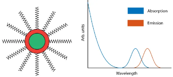
Figure 4. A) A diagram of a QD showing the core, shell, and surface ligands. B) Typical QD absorption and emission spectra.

(18)

18

1.4 The Monte Carlo Method

The Monte Carlo simulation method borrows its name from the famous Monte Carlo casino in Monaco. The general procedure is to simulate several trials of a process; in each trial, a random variable is drawn from a particular physical distribution, much like a spinning a roulette wheel and seeing where the roulette ball lands. This random variable determines the outcome of the process for that particular trial, and by averaging the results for several trials, a distribution of outcomes appears.18_{As the sample size of}

trials increases, the distribution of outcomes will approach the physically observed results of the process. For example, for the simple process of light transmitting through an interface, we can suppose that 100 photons impinge upon an interface from a material of index of refraction n1 to index of refraction n2. For each photon, the

probability of transmission is given by the Fresnel equations. In a Monte Carlo simulation of transmission, for each photon a random variable between 0 and 1 is generated. If this number is less than T, we count the photon as transmitted. If this number is greater than T, we count the photon as reflected. After 100 trials, the ratio of transmitted photons to total photons will resemble T.

For a relatively simple process like the example above, it is very simple to write out an analytic expression for the expected results – the physics is very well-known and

straightforward. However, for a more complicated process or series of processes, while the physics of individual segments may be well-known and simple, when taken as a whole it is intractable to write an analytic expression for the behavior of the system as a whole. For every random process in a series of processes, an analytic expression requires writing down an integral that averages over the probability distribution function (pdf) of the potential outcomes of that process. For the photophysics of an LSC19–22, by the time you take into account photons that are absorbed by a fluorophore and re-emitted to be captured by the solar cell, the minimum number of sub-processes that must occur for an efficiency greater than 0 to be achieved, 6 random processes occur, including

(1) whether a solar photon is transmitted into the waveguide or not,

(19)

19

(3) whether the fluorophore decays radiatively or not,

(4) the direction in which the fluorophore re-emits the photon,

(5) if the re-emitted photon reflects to remain within the waveguide or transmits through the top or bottom of the device, and

(6) how far the re-emitted photon travels within the waveguide before potential reabsorption events.

Then, if the photon can survive these 6 random processes, the solar cell captures it and we increment our tabulation of device efficiency. If we wanted to write down the

efficiency of this process in an analytic form, it would contain at least 6 nested integrals, each one with an ever-evolving pdf to weight them as the relevant parameters of the light within the device changes due to random events. Furthermore, the geometric constraints of the device are relevant to many of these processes, requiring us to keep track of 3 axes simultaneously, each one with its own set of integrals. Some of these properties occur on a spherical coordinate system, so integrals over pdfs with

trigonometric distributions will mix the 3 axes together and with trigonometric functions. On the other hand, the Monte Carlo method allows for rapid implementation of rather simple physical processes in a simulation that, if run for a long enough time, will

converge to the correct answer, while being highly adaptable to changing the underlying parameters. This adaptability makes Monte Carlo simulations very useful for predicting how changing a small feature of a system will change the overall behavior of the

system. This can be applied not only to changes in the physical realization of the system that is modeled, but to changes in the “rules” that underpin the physical workings of the system, in order to understand what about how the system works is important to the results. As an example, consider a thin waveguide of great lateral extent.

Figure 5. In a waveguide with a large geometric gain, photons may have to reflect several 10s of times to reach the end of the device.

(20)

20

A photon is emitted within this waveguide at a random angle between -90 to 90 degrees, and we are interested in the efficiency of the waveguide transmitting the photon all the way to the face on the far right. Above the critical angle, the photon has a chance of escaping but is not expected transmit through the top or the bottom face with 100% certainty. However, any photon emitted above the critical angle, in order to make it all the way to the collection face, must be reflected several 10s of times. For an angle 𝜃 > 𝜃_{𝑐𝑟𝑖𝑡𝑖𝑐𝑎𝑙}, 𝑃{𝑝ℎ𝑜𝑡𝑜𝑛 𝑖𝑠 𝑐𝑎𝑝𝑡𝑢𝑟𝑒𝑑 𝑏𝑦 𝑠𝑜𝑙𝑎𝑟 𝑐𝑒𝑙𝑙} < 𝑅𝑁_{, where N is the minimum number}

of reflection events. With 𝑁 > 50, as in [Figure XX] above, R can be as large as 0.9 and 𝑃{𝑠𝑢𝑟𝑣𝑖𝑣𝑎𝑙} < 1%. Due to the low probability of photons emitted above the critical angle surviving to the far end of the waveguide, rather than using the physical reflection probabilities, the Monte Carlo simulation can use the following:

𝑅 = {1, 𝜃 ≥ 𝜃𝐶𝑟𝑖𝑡𝑖𝑐𝑎𝑙 0, 𝜃 < 𝜃𝐶𝑟𝑖𝑡𝑖𝑐𝑎𝑙

Above the critical angle, total internal reflection occurs, and the photon can survive any number of reflection events. In the absence of re-absorption as in our example, these photons will reach the far end of the device. Below the critical angle, the number of reflection events required for capture is simply too many to have an appreciable chance of survival. By allowing photons to escape perhaps a few reflection events earlier than the correct physical model would suggest, our Monte Carlo simulation culls non-viable photons, thus speeding up the simulation. We might have discovered this by varying the implementation of reflection physics and noticing what variations do not change the results over a variety of conditions, and taught ourselves a lesson about what physical processes within such a device matter for efficient photon collection.

It is important to note that while an implementation of a non-physical process in a Monte Carlo simulation may not change the results for a specific distribution of interest,

another resulting distribution may change. If we were to look at not only what fraction of photons survived to the end of the device but also the average distance that photons travel down the device, then our non-physical implementation of reflection would not give an accurate result. For validation of a Monte Carlo simulation and its modeling of a physical process, it is always best to run checks using correct physical implementations of all sub-processes. One caveat to this rule is that it is impossible to prove the

(21)

21

knowledge of all physical laws, and therefore impossible to prove that a particular Monte Carlo simulation is a fully accurate model of the correct physical behavior of a system. Design of a Monte Carlo simulation will always consist of careful implementation and pruning of physical processes in order to best approximate our physical reality. By implementing finer and finer degrees of a physical model of the universe, a Monte Carlo simulation’s results may be slightly offset from the previous results, but not to an extent that the results will converge within for number of trials that can be simulated practically. In the use of Monte Carlo simulations, the scientist can chase perfection but it is not always wise.

(22)

22

1.5 Details of Monte Carlo Simulations of Luminescent Solar Concentrators

The details of a Monte Carlo Simulation of an LSC are not much more complicated than the example described in the preceding section in principle. The main physical

processes occurring in an LSC are transmission/reflection, absorption, and emission. Each of these three processes has a distribution of behavior for which the simulation will draw a random variable to sample appropriately. Due to the large number of random processes in series, a significant number of trials is performed to converge to the average simulation result.

The first step in performing a Monte Carlo simulation of an LSC is to build the LSC. The LSC is assumed to be a rectangular prism made of a stack of layers of identical lateral extent and varying thickness. An integrated single-layer LSC would have a single layer in this model and a thin-film LSC would have two layers: one for the waveguide layer, and a thinner one for the thin film of fluorophores. More complex LSCs are modeled by adding additional layers with different properties. Each layer has several properties indicated upon creation: an index of refraction, a thickness, an absorption spectrum, a quantum yield, and an emission spectrum. A waveguide layer in a thin-film LSC, for example, would have a constant zero absorption spectrum and an index of refraction of roughly 1.4-1.5, depending on the material simulated. For this description, we assume that scattering is negligible, but to simulate scattering a scattering spectrum would also be included.23

Once the LSC is constructed, the simulation proceeds by generating photons above the device with a trajectory toward the LSC and simulating the entire lifecycle of each photon one-by-one, drawing random variables from the appropriate distributions to simulate random behavior. For each photon, the simulated records whatever the desired metric is, and the result of the simulation is the distribution of this metric over the sample space of randomly-behaving photons. For example, if the figure being simulated is the efficiency of the LSC, then the simulation records whether each photon is captured by the solar cell or lost to any loss mechanism; then the simulated efficiency is the number of captured photons divided by the number of trials.

(23)

23

While simulating the lifecycle of a photon in an LSC, the photon’s wavelength, position, and trajectory are tracked throughout the entire simulation. The routine goes as follows:

1. A photon is instantiated above the device with a wavelength either

pre-specified or drawn from a distribution such as the solar spectrum. Its position and trajectory are set.

2. For the current layer the photon resides in, a penetration depth is drawn by comparing a random variable between 0 and 1 to the exponential cumulative distribution function (cdf) of the mean free path for the photon wavelength, calculated from the transmission spectrum.

3. Using the geometry of the device, the simulation traces the photon’s straight-line trajectory up to either the determined penetration depth or a collision with any interface, whichever comes first. If the penetration limit occurs first, then the photon is absorbed and go to step 5. If the collision point occurs first, the photon will either reflect or transmit off the interface and proceed to step 4. 4. For the photon’s trajectory and angle with the interface, the reflection and

transmission probabilities are calculated and compared to a random variable between 0 and 1 to determine which occurs. Snell’s Law determines the updated trajectory of the photon If the photon ends up outside of the device and moving away from it, the simulation records the photon as either lost out the top or the bottom face of the device, or captured out the side. If the photon remains in the same layer, the distance it traveled is subtracted from the balance of penetration depth before absorption and the simulation returns to step 3.

5. If absorbed, a random variable between 0 and 1 is drawn and compared to the QY of the fluorophore in that layer to determine if the fluorophore relaxes radiatively or not. If it does, a trajectory is drawn from a uniform distribution around all 4π of solid angle and a wavelength is drawn by comparing a random variable between 0 and 1 to the cdf of the fluorophore’s emission spectrum. Return to step 2.

(24)

24

In order to accomplish these simulations, there are two main code files. First, there is a file that defines the object of a concentrator. The methods of the concentrator class are grouped into two categories: the methods to build the concentrator to set it up for simulation trials and the methods to run trials of photons interacting with the

concentrator. The methods to build the concentrator include functions that add layers to the concentrator and determine the necessary cdfs from the experimental data sets. The methods that run trials of photon interaction with the concentrator include the propagation method and methods to keep track of information about each trial, such as if a photon is captured or lost or the wavelengths of fully transmitted photons. The second file to run these simulations is a script that implements the simulations

themselves. This file is where experimental data is loaded and cleaned up to be entered into the concentrator object. For example, if the experimental transmission spectrum goes to 100% at high wavelengths indicating the fluorophore does not absorb after a certain point but the emission spectrum of the fluorophore is non-zero above the highest wavelength for which transmission data is recorded, the transmission spectrum must be padded with 100% values at higher wavelengths, at least up to the highest emission wavelength of the fluorophore. If not, then when a photon re-emits with a wavelength above the highest in the absorption spectrum, the routine will crash as it is unable to determine the mean-free path for this wavelength.

(25)

25

1.6 Comparison of Luminescent Solar Concentrator Simulations and Experimental Measurements

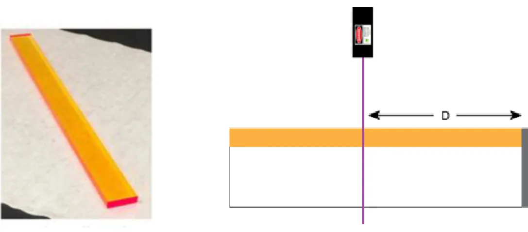
To verify the accuracy of the results of the LSC Monte Carlo simulations, several test case simulations were performed and compared to experimental results. A 30-cm by 3-cm thin-film LSC, using polymer-stabilized CdSe/CdS QDs developed by Odin Achorn as the fluopohores, was illuminated from above with a 405 nm laser at variable points along the top of the device. In three test cases, the flux of photons reaching a silicon solar cell was recorded versus the lateral distance between the solar cell and the laser illumination. In the first test case, there was an air gap left between the 3-cm side of the LSC and the solar cell. In the second test case, the solar cell was coupled to the side of the LSC. In the third test case, the solar cell was coupled to the side of the LSC and black tape was stuck all around the other 3 lateral faces of the LSC, so that any light reaching those sides is absorbed. Taken together, these tests show the effect of escape cone losses on the efficiency of photon collection in LSCs.

Figure 6. Left: Image of a device used in the experiment. Right: diagram of the laser illumination experiment. The violet line represents the laser illumination of the device, and the gray rectangle represents the silicon solar cell used to measure the photon capture

efficiency. D is the variable distance of the laser illumination from the solar cell.

CdSe/CdS QDs were chosen as the fluorphores not only to demonstrate their efficiency as polymer-stabilized fluorophores in an easily-fabricated thin-film LSC, but also

because their near unity QY and low reabsorption greatly reduce the magnitude of other loss mechanisms and highlight the role of escape cone losses. Additionally, these

(26)

26

features of CdSe/CdS QDs make their simulation excellent test cases, as the physics is relatively simple without as many reabsorption events occurring.

Simulations of the first experimental test case, with an air gap between the LSC and the solar cell, are essentially unmodified from section 1.5 using an initial wavelength

distribution of a delta function at 532 nm. For this test case and all test cases, the same absorption and emission spectra were assumed. The emission spectrum of the QDs in film was measured directly using a spectrometer, and the absorption spectrum was derived from the measured transmission spectrum of the device and the known polymer film thickness. After simulated photons pass through the side of the LSC nearest the solar cell, their trajectories were calculated outside of the solar cell and

reflection/transmission probabilities into the solar cell were calculated. In principle, this results in an LSC simulation that behaves like the face with the solar cell next to it has different reflection/transmission behavior than the other 3 lateral faces. Namely, this face has additional reflection due to photons reflecting off the solar cell and transmitting back into the LSC.

In simulations of the second experimental test case, all photons that hit the side of the LSC next to the solar cell are assumed to pass through because of the identical indices of refraction of the LSC and the coupled silicon solar cell.

In simulations of the third experimental test case, all photons that hit any lateral side of the LSC are assumed to pass through because of the identical indices of refraction. This is analogous to index-matching at one face, for which the number of photons passing through it is recorded, and total absorption at all other lateral faces, because index-matching at those faces causes total loss of all photons as total absorption would.

(27)

27

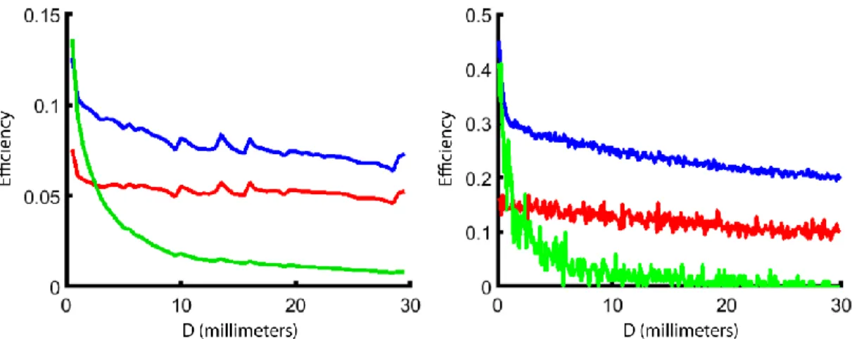
Figure 7. Left: Experimental photon capture efficiency vs. distance of illumination from the solar cell for three cases: air-gapped solar cell in red, index-matched solar cell in blue, and index-matched solar cell with black tape on all other faces in green.

Right: Simulated photon capture efficiency vs. distance of illumination from the solar cell for three cases: no index-matching in red, index matching in collection face only in blue, and index matching through all lateral faces in green.

Comparison of the experimental and simulated results show the shape of their curves to match closely. Systematic deviations in the experimental photon capture efficiency from smooth curves were found to be from non-uniform fluorphore films, noticeable by eye. Deviations from smooth curves in the results of Monte Carlo simulation are from sample noise due to running only 10,000 photon simulations per data point. This is evident in the increased noise in conditions leading to lower capture efficiencies, as these simulations have lower sample sizes and greater noise.

In both the experimental and simulated results, the green curves can be predicted almost purely from geometry. In both cases, they represent photons that are re-emitted by the fluorophore directly toward the face of the device that is coupled to the solar cell. The resulting efficiency is the fraction of a the solid angle of a sphere that projects onto a rectangle D cm away. The experimental results show that the blue and green curves should be roughly identical at the short endpoint, and with enough simulated photons, they would meet in the simulated data right below 0.5 efficiency. This is because when the illumination is right on the edge of the device, just under half of the emitted photons are emitted toward the face coupled to the solar cell. The steep drop-off of solar photon

(28)

28

capture efficiencies just above the low end of D occurs because as the illumination is moved away from the edge, the first photons that encounter the top, bottom, and sides of the device are emitted at high angles in the escape cone. The behavior of the red and blue curves at the high end of D, where a minimum solar photon capture efficiency is reached, is due to photons emitted below the angle of total internal reflection. These photons will always reach the face next to the solar cell and in the case of a solar cell index-matched to the device, will always be captured by the solar cell. The slow decline of the red and blue curves is due to the medium angles of re-emitted light that aren’t low enough to be totally internally reflected, but have an appreciable chance of being

reflected within the device. As D increases, these photons have to undergo an increased number of reflection events on average to be captured, and if any single transmission event occurs, that photon is lost. The result of this long, slow decline is that the size of a device can be increased substantially without a huge drop-off in device efficiency. Devices in which photons have to travel a maximum of 30 cm to be captured do not have much lower efficiencies than devices in which photons have to travel a maximum of 15 cm to be captured, so long as there is little self-re-absorption in the fluorophore layer.

(29)

29

1.7 Tandem Luminescent Solar Concentrators

Even with an efficient QD fluorophore such as polymer-stabilized CdSe/CdS QDs, an LSC with a single layer of fluorophore material will have losses due to transmission. In fact, incomplete light absorption is a consequence of the high Stokes’ shift in the QD system that helps to increase efficiency by reducing the self absorption of light re-emitted by the QD fluorophore. Even if the QD emission is right at the silicon bandgap, due to this Stokes’ shift and the minimal overlap between QD absorption and emission spectra, there is a range of wavelengths that are energetic enough to excite the silicon solar cell but redder than the QD can absorb.

One way of reducing the resulting transmission losses is via a tandem LSC design.24–26 A tandem LSC is and LSC that incorporates multiple fluorophore materials in multiple thin-film layers. In this case, we pair a QD fluorophore with a dye fluorophore. Dyes can be good fluorophore materials, but for different reasons from QDs. Organic days can have wide absorption spectra and absorb a lot of light at high concentrations, but they often have little Stokes’ shift and suffer from self-re-absorption due to a significant overlap of their absorption and emission spectra. By themselves, dyes are not

necessarily the best LSC materials. However, a second layer of fluorophore material containing a dye can help to boost the overall efficiency of a QD LSC. Any transmitted solar photon or re-emitted photon that would be lost out the bottom of the QD LSC has a chance of absorption by the dye fluorophore and subsequent capture by the solar cell. If the dye’s absorption spectrum does not overlap with the QD emission spectrum, then any light absorbed and re-emitted by the QD is left alone: this means that any solar photon that the QD-only LSC would collect, is also collected by this tandem QD-dye LSC. For such a device, the addition of a dye fluorophore layer only increases the overall solar photon collection efficiency.

(30)

30

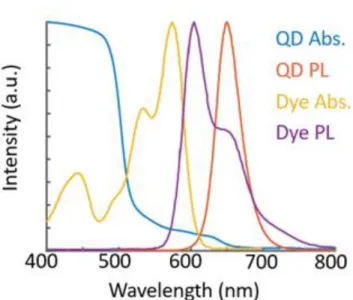
Figure 8. Absorption and emission spectra of CdSe/CdS QDs and Lumogen F red 300 dye. The dye absorption band, in yellow, fits between the absorption and emission spectra of the QDs. This increases the amount of light absorbed by the device, without interfering with the capture of photons re-emitted by the QDs.

The efficiency of a tandem QD-dye LSC was simulated using the Monte Carlo LSC simulation code described above. The dye was assumed to be Lumogen F red 300 and the QD was assumed to be polymer-stabilized CdSe/CdS QDs developed by Odin Achorn. Because re-absorption is increasingly detrimental in devices of greater total optical depth, the efficiency vs. distance from the edge of the device is plotted.

(31)

31

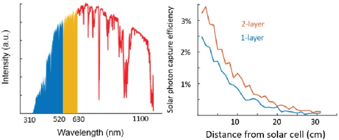
Figure 9. A) In red, the solar spectrum. In blue, available solar radiation for a QD LSC. In orange, additional solar radiation available in a tandem QD-dye LSC. B) The capture efficiency of solar photons in the 1-layer (QD-only) and 2-layer (QD-dye) devices as a function of distance from the solar cell. Note that the solar photon capture efficiency has all solar radiation in the denominator, even that which cannot excite the silicon bandgap without upconversion.

The band gap of silicon is roughly 1100 nm, and silicon solar cells will only capture photons with a wavelength of 1100 nm or lower. In order for silicon to capture lower energy photons, they must first undergo upconversion27–31, a process by which a material sequentially absorbs two photons, and then emits a single photon of greater energy. Compared to an LSC with just a QD layer, the proposed tandem QD-dye LSC can absorb nearly twice as much of the solar spectrum. The extra light absorbed increases the solar photon capture efficiency, but not nearly by the same factor as the increase in absorption. Photons absorbed by the dye layer are less likely to be collected by the device than those absorbed by the QD layer, owing to reabsorption of light

(32)

32

Chapter 2. J-aggregates

2.1 Background on Molecular Aggregates

Molecular aggregates are systems of identical molecules held together by non-covalent forces. In these systems, the excited states of individual molecules interact and mix to create collective excited states that delocalize across the entire aggregate.32_These

collective excited states are analogous to molecular orbitals formed by interaction of atomic orbitals, or the energy bands in semiconductors. In his seminal 1936 paper33_,

Jelley noted that in high concentration and in particular conditions the spectra of certain dye molecules changed in an unexpected way, narrowing and shifting to a longer wavelength. This observation is an effect of molecular aggregation of a particular type, known as J-aggregation. Another type of molecular aggregation, in which the dye absorption spectrum narrows but instead shifts to a shorter wavelength, is

H-aggregation. These spectroscopic changes occur due to the geometry of the ground state and excited state in the individual dye molecules and the geometry of the overall aggregate, and exist as a consequence of how the properties of the molecules cause themselves to be arranged.34,35_{These individual, identical molecules are often referred}

to as “monomers” because of the similarity to how monomer subunits of a polymer arrange together to form a larger system with emergent properties. This terminology, when applied to molecular aggregates, is strictly incorrect, because covalent bonds do not form between the molecules in molecular aggregates. Nevertheless, this

terminology is convenient to use.

Dye molecules include any molecules used industrially to dye textiles or other materials, and their properties in industry persist in their chemical study. First, a good dye must have a strong absorption peak in the visible spectrum, to be able to give a material a strong color with minimal dye used. In organic dyes, these strong absorption spectra often arise from conjugated double bonds that create an energy splitting between the molecule’s highest occupied molecular orbital (HOMO) and lowest unoccupied

molecular orbital (LUMO). The electronic structure of many of these dyes can be

(33)

33

exist, the most useful dyes that produce the purest colors in all conditions will behave as two-level systems. Secondly, industrial dyes contain side-chains, or substituent groups that do not make up the color center of the molecule. These side-chains are important for binding of the dye to textiles or other materials, and also key in the formation of molecular aggregates. Some families of molecular aggregates are formed by preserving the chromophore group of an organic dye molecule and varying the side-chain. For example, dyes based on isocyanine with varied side-chains include C8S3, C8O4, and others.36–40 The presence of these side-chains and how their interact both sterically with the side-chains of other molecules as well as with the electrostatic environment of the solvent and any dissolved ions is a major factor in the geometry of a molecular

aggregate system and therefore in that system’s spectroscopic properties.41–43

This work will mainly focus on J- and H-aggregates. J-aggregates we define as molecular aggregates that exhibit a redshifted absorption and emission spectrum

compared to the dye, and H-aggregates we define as molecular aggregates that exhibit a blue shift. Some authors are specific in defining J-aggregates as ones in which the electronic state with the greatest cross-section is also the state of lowest energy, but we will refer simply to any shift from the dye spectrum.34

(34)

34

2.2 Basic Physics of Molecular Aggregates

To understand the emergent properties of J- and H-aggregates, it is important to understand first the concept of a transition dipole. When a dye molecule that we shall consider an idealized two-level system is excited by absorbing radiation, the valence electron in the molecule transitions from the ground state to the excited state. This corresponds to a change in the electronic density. For an easy to conceptualize model, imagine the dye molecule’s frontier molecular orbitals to be like a particle in a box. There is one valence electron in a box with length roughly the length of the

chromophore region in the molecule. For pseudoisocyanine, this would be the

conjugated double-bond region between the heterocyclic rings. At the ground state, the electronic wave function looks like the fundamental note on a stringed instrument, or roughly like one half-period of a sinusoidal function: it is equal to zero at the ends for normalization, and it raises to a finite value in the middle. The excited state wave

function looks roughly like one full period of a sinusoidal function: over the left half of the box, it looks identical to a squished version of the ground state wave function, and over the right half of the box, it looks like the ground state wave function mirrored over the x-axis.

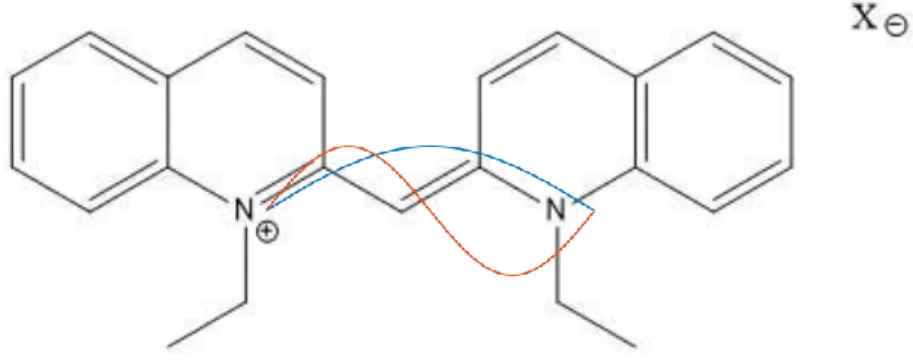
Figure 1. Diagram of pseudoisocyanine molecule and a rough estimation of the ground and first excited state wavefunctions, showing the origin of the transition dipole.

Naturally, by orthonormality of the particle-in-a-box wave functions, the product of either of these two wave functions with the adjoint of the other vanishes when integrated over the length of the box.44_{There is, however, a net movement of electron density: when}

(35)

35

distance from the center of the box, the result is a finite number. This is essentially the mathematical basis for excitation by a photon and illustrates the dipole character of the ground state-excited state transition. For an exact model of the electronic density, a similar computation for higher-order terms in the multi-pole expansion of the

electromagnetic interaction would show the quadrupole, octupole, etc. components.45

Here, we only consider the dipole moment both for illustration purposes and because for these elongated conjugated double-bond chromophore regions, the model that takes after the particle-in-a-box model is sufficient for many purposes.

It is important to distinguish these dipoles from the electric and magnetic dipoles that we traditionally discuss in physics. The dipoles of interest in molecular aggregates are transition dipoles that represent the dipole moment of the transition between the ground and excited electronic states in a molecule. Like electric dipoles, transition dipoles have a vector orientation and a dipole moment – the two values necessary to specify a

unique vector. Also like electric dipoles, transition dipoles can be described as a positive and a negative charge separated by a particular distance. Specifying the coordinates and magnitudes of these charges describes a unique dipole. While the electric charges of an electric dipole are physical quantities, the transition charges of a transition dipole are more of an abstract concept, being related to the amount by which the amplitude of the electron wave function around a particular point in the molecule increases or

decreases. In the example above, the locations of the transition charges are at the maximum positive and negative displacement of the excited state wave function, and their magnitudes would be related to the amplitude of the excited state wave function. This coupling model is the extended dipole model, for which the transition dipole moment, μ, is related to the transition charge, q, and charge separation, d, by

𝜇 = 𝑞 𝑑.

While electric dipoles have a strict positive and negative end, transition dipoles do not. By changing the phase of the excited state wave function 180 degrees, the positive and negative sides completely flip.

Neither the simple transition dipole model nor the extended transition dipole model fully describes the behavior of coupling between two molecules in a molecular aggregate. To

(36)

36

do so requires a treatment of all the individual atomic interactions for the entire aggregate. The simple dipole model is a convenient way to capture much of the behavior of the system and form an intuition for why the emergent properties of molecular aggregate systems occur.

(37)

37

2.3 Emergent Properties of Molecular Aggregates

When individual dye molecules form aggregates, they exhibit many emergent

phenomena. Many of these phenomena are spectroscopically observable, and can be traced back to the coupling of monomer excited states into a larger framework of delocalized excited states shared between multiple monomers. To illustrate the basics of this framework, consider two infinite or near-infinite linear aggregates. One of these aggregates is in the “card-pack” arrangement, where the dipoles are parallel to each other but not co-linear. An electronic state of this aggregate consists of giving the sign of each dipole, whether it is positive and pointing up, or negative and pointing down. The other aggregate is the parallel, co-linear case where each dipole’s tip and tail point directly at the neighboring dipoles. It is also possible to have a linear aggregate where each dipole makes an angle with the axis of the aggregate, but these two extremes help to illustrate the difference between J- and H-aggregates and their electronic structures. For these two aggregates, specification of the sign of every dipole fully describes an electronic state. For an aggregate of N molecules, there are N excited states. These states have 0 through N-1 nodes, where the sign flips from one dipole to the next. For the J-aggregate, when the wave functions of two adjacent dipoles have the same sign, the contribution to the total energy of the state is negative, because a positive transition charge at the tip of one dipole is pointing toward the negative transition charge at the tail of the next, and by Coulomb’s Law that is a negative interaction. For the H-aggregate, when the wave functions of two adjacent dipoles have the same sign, the contribution to the total energy of the state is positive, because the positive transition charges at the tips of the two dipoles are lined up, as well as the negative transition charges at the tails of the two dipoles. Therefore, the energies of the electronic states of the J-aggregate increase with an increasing number of nodes, while the energies of the electronic states of the H-aggregate increase with a decreasing number of nodes. For an infinite or near-infinite one-dimensional J-aggregate, the state with highest total dipole strength with the wave functions of all dipoles in phase has the lowest energy of all J-aggregate

electronic states. Conversely, for the same such H-aggregate the state with the greatest transition dipole strength and the excited state wave functions of all the monomers

(38)

38

aligned is the state with the highest energy. This is the origin of red-shift in J-aggregates and blue-shift in H-aggregates, as the absorption cross-section is directly proportional to the square of the transition dipole moment of each state.

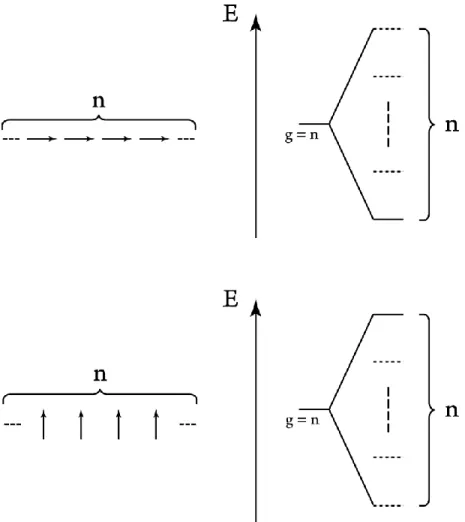
Figure 2. Top: A diagram of the transition dipoles of a 1-D J-aggregate containing n molecules and an energy diagram showing the n degenerate excited states splitting into n states with a spread of energy levels. Bottom: A diagram of the transition dipoles of a 1-D H-aggregate containing n molecules and an energy diagram showing the n degenerate excited states splitting into n states with a spread of energy levels. In both energy level diagrams, dashed lines represent states without any dipole moment and solid lines represent states that contain all the dipole moment of the aggregate.

(39)

39

2.4 Molecular Aggregates of Greater Dimensionality

For the case of linear molecular aggregates, the presence of a red-shift in J-aggregates and a blue-shift in H-aggregates is fairly straightforward. In a 2-D aggregate such as a planar aggregate or a tubular aggregate, the classification of J- or H-aggregate is not so simple.34,46,47_{Consider the case of an aggregate of molecules aligned on a 2-D grid in}

the x-y plane, with equal spacing along both axes. If the transition dipole moments align with the z-axis, then all interactions between molecules look like those of H-aggregates, and this in fact makes an H-aggregate. However if all the transition dipoles align with the y-axis, then each row of molecules looks like an H-aggregate and each column of molecules looks like a J-aggregate. In this case, it is ambiguous which type of

aggregate it is, depending on the exact parameters of the system. In this case, even if there is a red-shift present in the absorption spectrum, the state with the highest dipole moment might not be the very lowest in energy and if there is a blue-shift the

aforementioned state might not be the highest in energy. This means that the 2-D J-aggregate does not always look identical to the 1-D J-J-aggregate and the 2-D H-aggregate does not always look identical to the 1-D H-H-aggregate, spectroscopically. When the transition dipoles in a 2-D molecular aggregate are unaligned to any axis, the exact angle produced with the axis strongly determines whether coupling of adjacent monomers along a particular axis is negative or positive. The grid distance along each axis determines the overall magnitude of these couplings, as Coulomb’s law has a 1/r2

dependence. It is the balance of those negative and positive couplings that determines if the overall coupling in the system is negative, producing a J-aggregate, or positive, producing an H-aggregate.

(40)

40

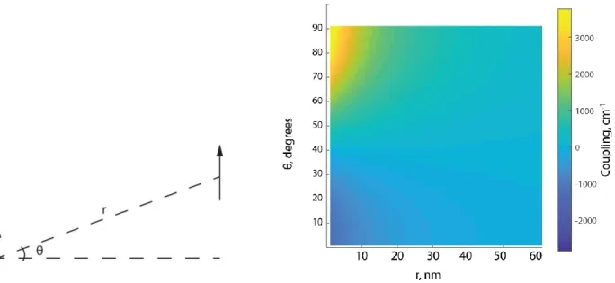
Figure 3. Dipole-dipole interactions as a function of the angle between them on the y-axis and the distance between them on the x-axis. The red line just below 40 degrees shows where the coupling switches from negative to positive.

Tubular aggregates are 2-D aggregates in which one axis wraps around to meet itself, while the other axis extends very far, forming a tube.48–50 The spectroscopic properties of these aggregates depend greatly on the number of molecules around the tube axis. In the limit of only one molecule around the tube, these converge to 1-D aggregates. In the limit of many molecules around the tube, these converge to planar 2-D aggregates.

(41)

41

2.5 Modeling J-aggregate Spectroscopic Properties

There are four basic steps in modeling the spectroscopic properties of molecular aggregates: defining the geometry of the aggregate, computing the Hamiltonian of the aggregate, diagonalizing the Hamiltonian, and computing the spectroscopic

observables.51–56 The exact method by which each of these steps is performed depends on the purpose of the modeling. No matter what the purpose of modeling is, however, one always starts from a place of assumptions or data. If someone wants to determine what the spectroscopic properties of molecular aggregate are from first principles, then they might simulate the chemical environment in which aggregates form, populate it with monomers, and run a molecular dynamics simulation.57_{If they formulate their model just}

right, they might see aggregates form and stabilize. Then the equilibrium state aggregate from their simulation provides the geometry for computation of the spectroscopic observables. In practice, this is difficult. This method is most likely to succeed when the monomers are arranged in a trial geometry that is the best guess for the system based on other observations, and even then the exact spectroscopic

observables are hard to reproduce. Another method of geometry determination is to start with a small set of assumptions based on spectroscopic and other observations, and then vary the remaining parameters to find what best fits the totality of known properties of the aggregate.

After determination of the aggregate geometry, the next step is to calculate the

Hamiltonian. The Hamiltonian is an N x N matrix, where N is the number of molecules in the system. The size of the Hamiltonian grows quite rapidly with N, so it is important to pick a value for N large enough such that the spectroscopic observables of interest converge sufficiently to the infinite or very large aggregate value, but small enough so that the given computational resources can perform all calculations efficiently. There are two sets of elements of the Hamiltonian: the diagonal elements, and the off-diagonal elements. The diagonal elements 𝑎_𝑖𝑖, 𝑖 ∈ {1,2,3, … 𝑁}, describe the excitation frequencies of the individual dye monomers. For homogeneous molecular aggregates of a single type of dye molecule without disorder, these elements will be identical. If there are multiple types of sites that dye molecules can occupy, if not all monomers are the same

(42)

42

molecule, or if there is disorder that breaks the symmetry of otherwise identical sites in the aggregate, then the diagonal entries will not be identical, and will instead come from one or more distributions of excitation frequency. While it is traditional to set the peak energy of the pdf of a molecule’s excitation frequency to that observed in the lab frame, this energy can also be set to 0 to be used as a reference point. The off-diagonal elements are the coupling terms between transition dipoles. The calculation of these terms depends on the coupling model used. Possible models include the simple dipole model and the extended dipole model, as mentioned previously. Another possible model is the transition density cube (TDC) model.58_{In this model, the space around the}

molecule is broken up into a grid of small cubes, each with a transition charge density from first principle calculations of the molecule’s ground and excited states. The coupling between two molecules is integrated over all pairwise interactions of grid points, yielding the overall coupling. The downside of the TDC method is that it is extremely computationally intensive. One approach that reduces the computational expense is to use the calculated TDC grid to assign a transition charge to every atom in the molecule, and instead calculate the coupling by summing up all pairwise interactions between atoms in the two molecules of interest. This can reduce the number of

calculations necessary to determine each coupling term by many orders of magnitudes while still maintaining a deeper level of interactions than the simple dipole or extended dipole models alone.

With the Hamiltonian in hand, the next step is to diagonalize the Hamiltonian to obtain the aggregate’s electronic states. If the Hamiltonian, H, is diagonalizable, there exists a matrix Q such that

𝐷 = 𝑄−1_{𝐻 𝑄,}

Where D is a diagonal matrix and Q is an invertible matrix, both with the same NxN dimensions of H. The columns of the resulting matrix Q represent the collective electronic excited states – or excitons – of the molecular aggregate, with each entry 𝑞_𝑖𝑗representing the coefficient of the excited state of the jth molecule in the ith exciton:

(43)

43 𝛹_𝑖 = ∑

𝑗

𝑞_𝑖𝑗𝜓_𝑗

Where 𝛹_𝑖 are the aggregate exciton wave functions, and 𝜓_𝑗 are the molecular excited state wave functions. Additionally, the matrix D will have on its diagonal the energies 𝜖_𝑖 of the aggregate exciton wave functions and be 0 everywhere else:

𝐷 = [𝜖1 ⋯ 0 ⋮ ⋱ ⋮ 0 ⋯ 𝜖𝑁 ]

Together, Q and D give a complete description of the electronic structure of the

aggregate. Many observables and other quantities derive from these variables such as the absorption spectrum, linear dichroism spectrum, and the participation ratio, which gives the average extent of exciton delocalization in an aggregate.

(44)

44

2.6 Coupling Models

As detailed above, the coupling model used will affect the off-diagonal terms of the Hamiltonian. Coupling models range from simple, lower order models that produce dipole coupling with as few variables as possible, to more complex, higher order models that require significant first-principles calculations to determine the appropriate

parameters. While simpler models may require less computational resources, they fail to replicate the coupling terms of more sophisticated models, especially at short distances. Consider the difference between the simple dipole and extended dipole coupling models shown below. The plots in Figure 4 show the coupling strength between two dipoles as a function of distance and angle of separation, as indicated in subfigure A. Subfigures B and C demonstrate that coupling models that are only slightly different can disagree in the magnitude and even sign of the coupling for a range of angles and distances. In a 2D aggregate where each dipole interacts with several neighbors at several different angles, this can be the difference between the overall coupling in an aggregate being negative, producing a redshift and nominal J-aggregate, and the overall coupling in an aggregate being positive, producing a blueshift and

nominal H-aggregate. Therefore, careful selection of the coupling model is very important for predicting the experimentally observed aggregate properties.

(45)

45

Figure 4. Comparison of the simple dipole coupling model (left) and extended dipole coupling model (right). Plotted is the coupling energy in cm-1_{as a function of the angle between}

dipoles on the y-axis and the distance between them on the x-axis. The lines in red show when the coupling switches from negative to positive. The differing models predict this switch to occur at very different angles, showing how important the coupling model is in accurately calculating the Hamiltonian of a molecular aggregate.

(46)

46

2.7 Disorder

Thus far in this chapter, molecular aggregates have been assumed to have perfect symmetry with exactly-defined coordinates for every molecule. In reality, each molecule does not position or align perfectly according to the assumed average coordinates and orientation. This results in disorder of both the diagonal and off-diagonal elements of the Hamiltonian.59_{The diagonal elements, which represent the individual excitation}

energies of each molecule, will vary within a distribution as the individual electronic environment seen by each molecule varies. Similarly, the off-diagonal elements, which represent couplings between molecules, will vary within a distribution as the individual distances and angles between dipoles vary. Depending on which elements the disorder occurs in, it is either diagonal or off-diagonal disorder. In J-aggregates, disorder causes a redshift and broadening of the absorption spectrum, while in J-aggregates it causes a blueshift and broadening. This effect are apparent in Figure 5 below, and is similar whether the disorder is diagonal or off-diagonal disorder. Because they are essentially equivalent, disorder is frequently modeled to be diagonal disorder only.

Figure 5. Effect of disorder on absorption spectrum of molecular aggregates. As the disorder increases from 400 to 500 to 600 cm-1_{, the spectrum redshifts and broadens.}

Reprinted (adapted) with permission from Doria et. al. Photochemical Control of Exciton Superradiance in Light-Harvesting Nanotubes. ACS Nano 2018, 12 (5), 4556– 4564.. Copyright 2018 American Chemical Society.

When modeling diagonal disorder in a molecular aggregate, an obvious choice for the distribution of individual energies is the Gaussian distribution. Since the solvent baths and aggregates themselves contain many atoms and bonds, it is sensible to apply the central limit theorem to the large number of interactions that may cause disorder and assume a Gaussian result. However, this is not always the case, as molecular