Use of Decision-Tree Induction for Process Optimization and Knowledge Refinement of an Industrial Process

(1)

Publisher’s version / Version de l'éditeur:

Journal of Artificial Intelligence for Engineering Design, Analysis and Manufacturing, AI EDAM, 1994

READ THESE TERMS AND CONDITIONS CAREFULLY BEFORE USING THIS WEBSITE.

https://nrc-publications.canada.ca/eng/copyright

Vous avez des questions? Nous pouvons vous aider. Pour communiquer directement avec un auteur, consultez la Questions? Contact the NRC Publications Archive team at

PublicationsArchive-ArchivesPublications@nrc-cnrc.gc.ca. If you wish to email the authors directly, please see the first page of the publication for their contact information.

This publication could be one of several versions: author’s original, accepted manuscript or the publisher’s version. / La version de cette publication peut être l’une des suivantes : la version prépublication de l’auteur, la version acceptée du manuscrit ou la version de l’éditeur.

Access and use of this website and the material on it are subject to the Terms and Conditions set forth at

Use of Decision-Tree Induction for Process Optimization and Knowledge Refinement of an Industrial Process

Famili, Fazel

https://publications-cnrc.canada.ca/fra/droits

L’accès à ce site Web et l’utilisation de son contenu sont assujettis aux conditions présentées dans le site LISEZ CES CONDITIONS ATTENTIVEMENT AVANT D’UTILISER CE SITE WEB.

NRC Publications Record / Notice d'Archives des publications de CNRC:

https://nrc-publications.canada.ca/eng/view/object/?id=2a3ba591-edfe-4d5c-ace9-bc4e67c5441d https://publications-cnrc.canada.ca/fra/voir/objet/?id=2a3ba591-edfe-4d5c-ace9-bc4e67c5441d

(2)

List of Tables

1. Examples of some facts that are included in the domain model 2. Examples of rules that are included in the domain model 3. Examples of rules generated for centr-kk-postform high 4. (a, b, and c) Examples of rule reduction

5. An example of a recommendation 6. (a and b) Examples of rule refinement 7. (a and b) Examples of induced rules 8. (a and b) Examples of rule refinement

(3)

List of Figures

1. The architecture of the intelligent supervisory system 2. The ECM process

3. A portion of the causal model of the ECM process parameters

4. A portion of the causal model with the relationships between preform and postform parameters 5. An example of a decision tree

(4)

Table 8 (a and b). Examples of rule refinement Rule

If

Leading-edge-dd-preform is more than 0.08695 and Mid-centre-dd-preform is more than 0.0735

Then

There will be the problem of center-kk-low

(a) Rule

If

or

Center-kk-preform is less than -0.54505 Then

(5)

Table 7 (a and b). Examples of induced rules

subspace centr-kk-lo: rule 1

le-dd-0 is more than 0.08695 mid-c-dd-0 is more than 0.07305

coverage 100.0% (train) 100.0% (test) error rate 0.0% (train) 0.0% (test)

(a) rule 1

centr-kk-0 is less than -0.54480 coverage 92.0% (train) 92.0% (test) error rate 2.2% (train) 4.3% (test) rule 1

centr-kk-0 is less than -0.54505 coverage 82.4% (train) 62.5% (test) error rate 0.0% (train) 0.0% (test)

(6)

Table 6 (a and b). Examples of rule refinement

Rule If

There is the problem of trailing-edge-ff-low Then

Pressure-in-actual should be more than 202 (a)

Rule If

Pressure-in-actual should be more than 203 (b)

(7)

Table 5: An Example of a Recommendation

variable influences suggestion

(8)

Table 4- Continued (a, b, and c). Examples of rule reduction

subspace mid-dd-hi: rule 1

plat-in-conc-0 is more than -42.38720 mid-dd-0 is less than 0.13420

rule 1

chord-ff-0 is less than 1.03595 sum-chord-0 is more than 3.09970 mid-dd-0 is more than 0.13770

plat-out-conv-le-0 is more than 0.01015 coverage 20.0% (train) 11.1% (test) error rate 0.0% (train) 0.0% (test)

(9)

Table 4 (a, b, and c). Examples of rule reduction

plat-in-conv-0 is less than -42.87760 le-dd-0 is more than 0.08855

rule 1

a )

subspace te-ff-lo: rule 1

p-in-act is less than 202.26500 shuttle-num is not 5

warp-kk-0 is more than -0.79905 coverage 50.0% (train) 20.0% (test) error rate 0.0% (train) 0.0% (test)

rule 1

p-in-act is less than 203.50000

(10)

Table 3. Examples of rules generated for the centr-kk-postform high

subspace centr-kk-hi: rule 1

p-out-act is less than 73.41000 coverage 94.7% (train) 73.7% (test) error rate 0.0% (train) 0.0% (test)

rule 2

p-out-act is more than 73.41000 le-dd-0 is more than 0.08370

coverage 5.3% (train) 21.1% (test) error rate 0.0% (train) 0.0% (test) combined rules

(11)

Table 2. Examples of rules that are included in the domain model Rule If Gas-level > x1 and Electrolyte-temp > x2 Then Electrolyte-resitivity Constant Rule If Center-kk is high or Center-kk is low Then Center-kk-perform should be > -0.54505 Center-kk-preform should be < -0.52525

(12)

Fact (center-kk-postform high -0.50) and (center-kk-postform low -0.52) Fact (gap-voltage on-time 18) and (gap-voltage off-time 17.5)

(13)

T = Target R = Rule Coverage = Error Rate = | T

∩

R | | T | | R — T | | T

∩

R | T R

(14)

Figure 5. An example of a decision tree False

False True

center-kk-postform will be above the upper limit

center-kk-postform will be below the upper limit center-kk-postform will

be above the upper limit

le-dd-preform > 0.0837 True

(15)

Figure 4. A portion of the causal model with the relationships between pre-form and postpre-form parameters

le-dd-0 centr-dd-0 centr-kk-0 plat-out-conv-le-0

le-dd-hi centr-kk-lo centr-dd-lo warp-kk-lo mid-dd-hi centr-kk-hi

le-dd-lo

preform parameters

postform parameters

(16)

Figure 3. A portion of the causal model of the ECM process parameters feed rate voltage inlet

pressure

inlet temperature concentration of

electrolyte

process parameters _{set up parameters} current

density gap flow rate

electrolyte velocity electrolyte conductivity operating temperature gas portion of electrolyte

positive change increase positive change decrease

(17)

(18)

Figure 1. The architecture of the intelligent supervisory system

IMAFO

Expert System

Reasons for Failed Plans

Industrial Process

Execute Succeeded Plan Operators/ Engineers

- Analysis of Process Information - Advice to Operators/Engineers Inference Mechanism Advice Generator Knowledge Base Domain Specific Knowledge Planning Information Execute Succeeded Plan Execute Plan Process Monitoring Module Data Conversion Module Data Collection Schedule Learning

Mechanism Initialization_Mechanism

User

Interface _GeneratorRule

Process Knowledge User Interface Setup Information Failed • • • Planning & Execution Information

(19)

Biography

A. (Fazel) Famili is a Senior Research Officer at the Knowledge Systems Laboratory of the Insti-tute for Information Technology of the National Research Council of Canada. Dr. Famili received his M.S. from The Ohio State University and his Ph.D. from Michigan State University. Prior to joining NRC (in 1984), he worked for industry for three years. His current research focuses on Machine Learning, Expert Systems, Applications of A.I. in Manufacturing, and Intelligent Super-visory Systems. He has published or has been the co-author of several articles in these areas and edited (with Steve Kim and Dana Nau) the AI Applications in Manufacturing book that was pub-lished by MIT/AAAI press in 1992. He is also in the editorial board of two scientific journals and is a member of AAAI.

(20)

Turney, P. and Famili, A. 1992. Analysis of induced decision trees for industrial process optimiza-tion, Proceedings of the 6th International Conference on Systems Research, Informatics and Cybernetics, pp. 19-24.

Widmer, G., Horn W., and Nagele, B. 1992. Automatic Knowledge Base Refinement: Learning from Examples and Deep Knowledge in Rheumatology, Report No. TR-92-16, Austrian Research Institute for Artificial Intelligence.

Wilkins, D.C. 1988. Knowledge Base Refinement using apprenticeship learning techniques, Sev-enth National Conference on Artificial Intelligence, Vol. I, pp. 646-651, Morgan Kaufmann Los-Altos, California.

Wilkins, D.C. 1990. Knowledge Base Refinement as Improving an Incorrect and Incomplete Domain Theory, Report No. UIUCDS-R-90-1585, University of Illinois, Urbana, IL.

Wylie, R.H. and Kamel, M. 1992. Model-based knowledge organization: a framework for con-structing high-level control systems, Expert Systems with Applications, 4(3); 285-296.

(21)

Politakis, P. and Weiss, S.M. 1984. Using empirical analysis to refine expert system knowledge-bases, Artificial Intelligence, 22 (1), 23-48.

Quinlan, J.R. 1983. Learning efficient classification procedures and their application to chess end games. In J.G. Carbonell, R.S. Michalski, and T.M. Mitchell, Eds. Machine Learning: An Artifi-cial Intelligence Approach, Volume I, pp. 463-482. Morgan Kaufmann, Los Altos, California. Quinlan, J.R. 1986. Induction of decision trees. Machine Learning, 1(1), 81-106.

Quinlan, J.R. 1987a. Simplifying decision trees. International Journal of Man-Machine Studies, 27(3), 221-234.

Quinlan, J.R. 1987b. Generating production rules from decision trees. Proceedings of the Tenth International Joint Conference on Artificial Intelligence, pp. 304-307. Morgan Kaufmann Los Altos, California.

Quinlan, J.R. 1993. C4.5: Programs for Machine Learning, Morgan Kaufmann Los Altos, Cali-fornia.

Risko, D.G. 1989. Electrochemical Machining, SME Technical Paper EE-89-820, Society of Manufacturing Engineers, Dearborn, MI.

Schank, R.C. 1991. Where’s the AI?, AI Magazine, 12 (4), 38-49.

Segre, M.A. 1991. Learning how to plan, Robotics and Autonomous Systems, 8(1-2): 93-111. Sriram, D. 1990. Computer-aided Engineering: The Knowledge Frontier (Volume I: Fundamen-tals), Course notes distributed by the author, Intelligent Engineering Systems Laboratory, MIT, Cambridge, MA.

(22)

Ginsberg, A., Weiss S. M. and Politakis, P. 1988. Automatic knowledge base refinement for clas-sification systems, Artificial Intelligence, 35 (2), 197-226.

Holder, L.B. 1990. Application of machine learning to the maintenance of knowledge base perfor-mance, Proceedings of the Third International Conference on Industrial and Engineering Appli-cations of AI and Expert Systems. pp. 1005-1012.

Indurkhya, N. and Weiss, S.M. 1991. Iterative rule induction methods, Journal of Applied Intelli-gence, 1, 43-54.

Garrett P., William Lee C., and LeClair, S.R. 1987. Qualitative process automation vs. quantita-tive process control. Proceedings of the American Control Conference, pp. 1368-1373.

LeClair, S.R. and Abrams F. 1988. Qualitative process automation. Proceedings of the 27th IEEE Conference on Decision and Control, pp. 558-563.

Michalski, R.S. 1986. Understanding the nature of learning: issues and research directions. In J.G. Carbonell, R.S. Michalski and T.M. Mitchell, Eds. Machine Learning: An Artificial Intelligence Approach, Volume II, Morgan Kaufmann, Los Altos, California.

Mitchell, T.M. 1982. Generalization as search, Artificial Intelligence, 18 (2), 203-226.

Mittal, S. and Frayman, F. 1989. Towards a generic model of configuration tasks, Proceedings of the Eleventh International Joint Conference on Artificial Intelligence, pp. 1395-1401, Morgan Kaufmann, Los Altos, California.

Nedelec, C. and Causse, K. 1992. Knowledge refinement using knowledge acquisition and machine learning methods, In T. Wetter et al., Eds. Current Developments in Knowledge Acquisi-tion-EKAW ‘92, Springer-Verlag, Berlin.

(23)

Acknowledgments

Collaboration of the General Electric Canada (Aircraft Engines) in this research project and the special help of Denis Lacroix, Jean-Claude Fagando, Paul Gregoire, Maurice Oullet, and Mario Alain, all of the General Electric plant in Bromont, Que., are greatly appreciated. The authors also would like to thank Peter Clark and Evelyn Kidd of the National Research Council Canada, for their comments on an earlier version of this paper.

References

Barbehenn, M. and Hutchinson, S. 1991. An integrated architecture for learning and planning in robotic domains. ACM SIGART Bulletin, 2(4), 29-33.

Cheng, J., et al. 1990. Expert system and process optimization techniques for real-time monitor-ing and control of plasma processes. Proceedmonitor-ings of SPIE, Vol. 1392, 373-384.

Craw, S. and Sleeman, D. 1990. Automating the refinement of knowledge based systems, Pro-ceedings of the Ninth European AI Conference, pp. 167-172.

De Barr, A.E. and Oliver, D.A. 1968. Electrochemical Milling, MacDonald, London.

Draper, N.R. and Smith, H. 1966. Applied Regression Analysis, John Wiley & Sons Inc., New York, N.Y.

Famili, A. and Turney, P. 1991. Intelligently helping human planner in industrial process plan-ning. AIEDAM, 5(2), 109-124.

Faust, C. L. 1971. Fundamentals of Electrochemical Machining, The Electrochemical Society, N.J.

(24)

covered knowledge into an expert system to give advice to the operators and engineers on how to solve a problem has been identified. Following is a brief description of two of them:

1. A user assistant expert system to filter the output of the learning system, to find the best set of rules that are generated and to suggest ways to improve inferior rules. For example, the expert system may suggest that the user should collect more observations, gather more measurements for each observation, or obtain a better balance of examples and counter-examples of a given prob-lem.

2. An expert system to model various aspects of a particular process. This system will have a Pro-cess Database, containing the ranges of proPro-cess variables (e.g., minimum, maximum, and nomi-nal), the ranges of final product variables, and required process materials. It will also have a Process Knowledge Base, containing rules for managing a process and predicting problems, based on the causal interactions among the variables.

(25)

this application:

1. Decision-tree induction is a useful method for analyzing data and discovering the reasons for failed productions. However, all the rules generated may not be applicable to a particular process. A method must be developed to summarize the results into a set of rules that are more comprehen-sible by the operators and engineers. We developed a method that we introduced in this paper. 2. Decision-tree induction assists in discovering both the attributes that are relevant to a problem and the particular values that are significant to the process. Both the relevant attributes and the predicted values can be used to build a domain model of the process.

3. Even when a process is optimized, decision-tree induction can be used to refine and update the domain model for various applications of a particular process. A causal model, for example, can be expanded to incorporate knowledge about various aspects of a process.

4. Without learning techniques, process optimization and knowledge refinement must be done by process engineers and technicians whose knowledge may be not be accurate and whose answers for failed operations may not be consistent. The approach described here has proven that learning techniques can support process optimization and knowledge refinement. Four other applications in which IMAFO was applied for process optimization of semiconductor manufacturing supports this conclusion.

5. An finally, the results of this work can be applied in qualitative process automation (LeClair and Abrams, 1988; Garrett, William Lee, and LeClair, 1987) where development of domain mod-els would enable process engineers to control complex systems more efficiently. This is done when a domain model is used to interpret the sensory data in order to construct or refine a process plan in real-time.

Our current research is focussed on knowledge refinement and combining learning with expert systems. A number of options to enhance our learning system (IMAFO) and to structure the

(26)

dis-________________________________________ Approximate Location of Table 7 (a and b) ________________________________________

________________________________________ Approximate Location of Table 8 (a and b) ________________________________________

7.0 Conclusions and Future Work

We have presented a method to apply decision-tree induction for process optimization and knowl-edge refinement of a complex industrial process. We have also proposed an architecture to com-bine learning and expert system technology to achieve the following goals:

1. extraction of knowledge from data, to assist operators and engineers to determine why some productions fail

2. structuring and refinement of discovered knowledge to provide support for consistent planning and decision making

Our learning system, IMAFO, had originally been tested with simulated data and the results were reported in an earlier paper (Famili and Turney, 1991). Part of this paper includes the results of applying IMAFO to a real application. Following are our conclusions about applying IMAFO to

(27)

parameters that do not meet the specifications).

________________________________________ Approximate Location of Table 6 (a and b) ________________________________________

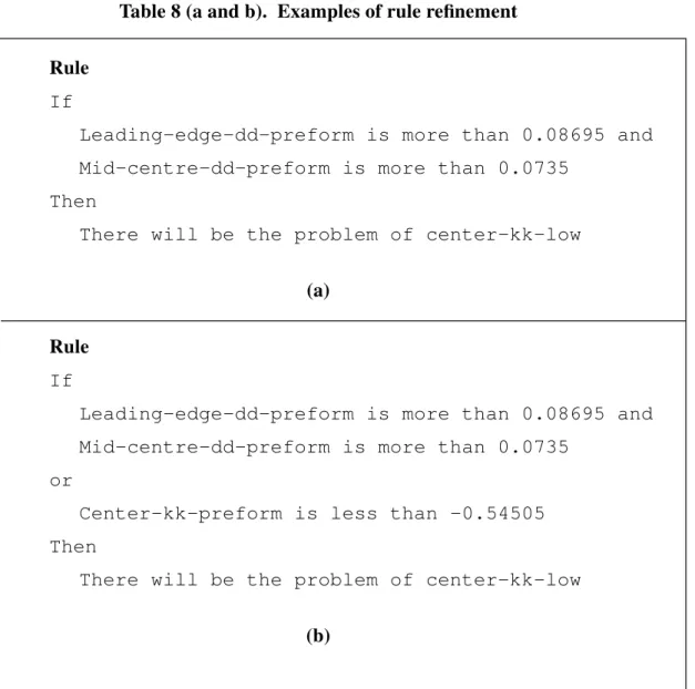
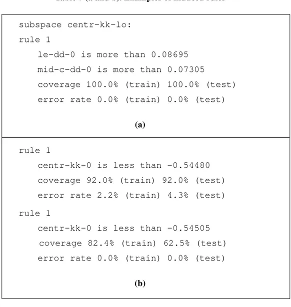
The second example discussed here is based on the causal model illustrated in Figure 4. In this example, three rules generated through decision-tree induction for one problem are used to build and refine a new rule to be used for process management. Table 7 shows the three rules. These three rules were chosen simply because their performances are very good. The rule in Table 7-a can be interpreted as “if le-dd-0 > 0.08695 and mid-c-dd-0 > 0.07305, then there will be the prob-lem of centr-kk-lo”. This rule can be converted to the first rule in Table 8-a. However, two more rules, given in Table 7-b, are also available for this problem. These rules report that “if centr-kk-0 < - 0.54480 or - 0.54505, then we will have the problem of centr-kk-lo”. To use the values of centr-kk-0, the conservative answer should be the smallest of the two (- 0.54505). Therefore, the rule in Table 8-a is updated to the rule in Table 8-b. The result is a new rule that can be used for process management. This rule predicts that the problem center-kk-low may be either due to com-bination of the leading-edge-dd-preform being more than 0.08695 and mid-center-dd-preform more than 0.0735 or because of center-kk-preform being less than - 0.54505.

(28)

6.1 Examples

In this section, two examples are given to further discuss how process optimization and knowl-edge refinement are achieved by applying the knowlknowl-edge discovered through decision-tree induc-tion. Mitchell (1982) and Politakis and Weiss (1984) suggest two forms of knowledge refinements: generalizations and specializations. This assumes that the knowledge base consists of production rules. Refinement in the form of generalization is accomplished by deleting or mod-ifying a proposition on the left-hand side of the rule or by raising the confidence factor associated with the conclusion of the rule. Specialization, however, involves modifications to one or more rules that make it harder for the conclusion(s) of the rule to be accepted at any given case. This is accomplished by adding or modifying a proposition on the left-hand side of the rule(s) or by low-ering the confidence factor associated with the conclusion of the rule.

It is assumed, here, that process optimization and knowledge refinement are not independent of each other. In other words, both the cause of the problem due to certain process or preform vari-ables and proper values for the same varivari-ables are selected from the rules generated through deci-sion-tree induction. For example, looking at the first rule in Table 4-b, if the second and the third variables are ignored (shuttle-num and warp-kk-0), the rule given in Table 6-a can be defined. This rule simply suggests that to solve the problem of te-ff-lo (one of the post-form problems), the p-in-act (the actual pressure of electrolyte when it enters the ECM chamber) should be more than 202. Rules of this type are verified by the domain expert before being included in the domain model. However, when the same variable is reported in a second rule, in Table 4-b, (which hap-pened to have a much better coverage, 100%, and error rate, 0%), the rule structure in Table 6-a is modified to Table 6-b. The suggested value of the actual pressure is now 203 instead of 202. Note that in both rules of Table 4-b, p-in-act is the first variable that was selected for the decision tree. In a more complex rule (of the type shown in Table 6), the ‘If’ part of the rule contains a conjunc-tion of predicate clauses that essentially looks for certain features about the preform or process variables in the model while the ‘Then’ part of the rule contains one or more problems (postform

(29)

Knowledge acquisition of expert systems is usually divided into two stages. In phase one, knowl-edge engineer(s) build a rough knowlknowl-edge base from the available sources such as domain experts, manuals, and textbooks. In the second phase, which is usually called knowledge base refinement, the initial knowledge base is progressively refined into a high-performance knowledge base. Referring to Figure 1, phase one consists of building most of the domain-specific knowledge and the major component of the process knowledge. Phase two will then include refinement of domain-specific knowledge and completion and gradual refinement of process knowledge.

Knowledge refinement can be thought of an optimization problem in which one starts with a pro-posed general solution to a given set of domain problems and the goal is to refine the knowledge base so that a superior solution is obtained (Ginsberg et al. 88). Refinement of the domain knowl-edge is an important task. This is because an initial knowlknowl-edge base is unlikely to perform ade-quately for all applications of a given domain. Refinement is therefore required and may consist of eliminating chunks of knowledge or modifying portions of rules/facts that already exist in a knowledge base. A solution generated as a result of knowledge base refinement will be a working knowledge base that may only require minor adjustments, i.e. one can assume that the rules incor-porated into the refined knowledge base are basically sensible propositions concerning the prob-lem domain.

In most process optimization applications certain aspects of the process are known a priori. The main task is therefore to find the best set of process parameters using the most appropriate tech-niques. Cheng et al. (1990) used a combination of decision-tree induction, response surface meth-odology, simulation, and sequential process optimization for real-time monitoring and optimization of a microfabrication process. We are mainly interested on using decision-tree induction for completion and further refinement of the domain model. This is done through con-tinuous use of the learning system (IMAFO) to analyze data from the ECM process and to refine or update the domain model until it is complete.

(30)

________________________________________ Approximate Location of Table 5

________________________________________

6.0 Process Optimization and Knowledge Refinement

The key to the performance of any process is proper optimization, acquisition, and refinement of domain knowledge. Process optimization and knowledge refinement play an important role in the performance of knowledge based systems. This is because an optimized process will result in an accurate domain model which is crucial to the solutions given by an expert system and to the suc-cess of a knowledge based approach. This section discusses how decision-tree induction can be applied to process optimization and knowledge refinement. An example is given in which a por-tion of a knowledge base is refined using the discoveries made through decision-tree inducpor-tion. The optimization task may involve definition of various process constraints or minimality/maxi-mality conditions on a feature of the solution (knowledge expansion). In these applications, pro-cess optimization problems may therefore be classified as problems in which variants of hill-climbing procedures are used. The analogy is as follows: similar to hill hill-climbing, at each cycle of knowledge refinement, the current state of the process knowledge base is evaluated. The heuristic function is applied to each of the successors, and the one with the best heuristic value becomes the new current state, replacing the previous one.

In building the domain model of a process, if an empirical model or an accurate physical model of the process is not available, response surface methodology may be used. This will result in con-structing an approximate model of the process using statistics (Draper and Smith, 1966). How-ever, completion of a domain model in a complex process may require other tools or techniques.

(31)

The above steps were followed for two reasons. First, to provide useful knowledge in the form of rules to the operators so that they can optimize the operation. Second, to verify this information with the domain experts and include that in a domain model to build an expert system for future process set up and problem solving. These steps can be easily automated. The best approach is to incorporate them into an expert system.

5.3 Performance Analysis

The final stage of the analysis, discussed in Section 5.2, had a major influence on the way that the results of the analysis were given to the operators. This is explained below:

1. The first step (elimination of rules based on the coverage, error rate and complexity) resulted into a reduction of about 47%, to a total of 171 rules. These were rules that were reliable and the engineers could simply read and interpret them.

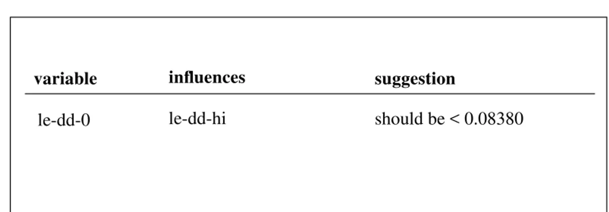
2. The second step (reduction based on the occurrence of parameters in the rule) resulted in even further reduction of the 171 rules to 46 rule sets. These rule sets were used to prepare the final summary that consisted of 10 recommendations. An example of a recommendation is given in Table 5.

The reduction achieved on the entire rule set, in two steps, was therefore about 97% (from 320 rules to 10). This helped the process engineers and operators to optimize the process in two ways: 1. All the recommendations for the preform parameters were applied by the group who were responsible for forging (the preform measurements were made by this group).

2. All the recommendations for process parameters were applied by the ECM operators and tech-nicians who were responsible for the ECM operation, final measurements and quality control.

(32)

ferent and both rules predict the problem, if the value of the parameter exceeds a given number, then the smaller value is taken as a suggestion for future operation. For example, in Table 4-a, one rule predicts the problem when le-dd-0 is more than 0.08855 while the other predicts the same problem when le-dd-0 > 0.08695. Our conclusion will be a new rule with the value of 0.08695 for le-dd-0 as a suggestion for future operation.

(ii) When the value of a single parameter reported in two rules (of a single class of problem) is different, one value is more than the other, both rules predict the problem if the value of the parameter is less than a given number, then the larger value is taken as a suggestion for future operation. For example, in Table 4-b, one rule predicts the problem when p-in-act < 202.265 while the other predicts the same problem when p-in-act < 203.500. Our conclusion will be a new rule with the value of 203.500 for p-in-act as a suggestion for future operation. (Note that the two rules in Table 4-b comes from two separate batches of data).

(iii) When the value of a single parameter reported in one or two rules (of a single class of prob-lem) is different and one rule predicts the problem if the value of the parameter is less than a given number while a second rule (or the same rule) predicts the problem if the value of the parameter is more than a given number, then the range is taken as a suggestion for future operation. For exam-ple, in Table 4-c, first rule predicts the problem when mid-dd-0 < 0.13420 while the other rule pre-dicts the same problem when mid-dd-0 < - 0.13770. Our conclusion will be a new rule with the optimum value of mid-dd-0 between 0.13420 and 0.13770 as a suggestion for future operation.

________________________________________ Approximate Location of Table 4 (a, b, and c) ________________________________________

(33)

________________________________________ Approximate Location of Figure 6 ________________________________________

5.2 Summarizing the Results

The results of the analysis were over three hundred rules, far more than what operators or engi-neers could use. These rules were analyzed to further reduce them to a smaller set of recommen-dations. The following steps were taken to summarize the results:

1. Elimination of certain rules based on one of the following three criteria:

(i) Coverage: all the rules with a coverage on either the training or testing set of less than 10% were deleted.

(ii) Error rate: all the rules with an error rate of more than half the coverage were eliminated (e.g. if the coverage is 60%, then the error rate must be less than 30%).

(iii) Complexity: all the rules with more than four variables were also deleted (e.g. in Table 3, the first rule has one variable and the second rule has two variables).

2. Reduction of some additional rules by focussing on parameters that occurred in two or more rules, generated from two or more batches of data. This was based on the assumption that when a parameter is discovered twice, using separate batches of data, it must have an important role in the physical process that caused the given rejection problem. This step may happen in three different forms:

(34)

dif-all 52 classes. The results of the analysis were therefore 52 different decision trees (for each batch of data), one for each class of problems.

The analysis involved conversion of decision trees into rules (Quinlan 1987a, 1987b), since we have found that rules are easier to interpret and apply. The results of the analysis also included sta-tistics on the success and failure of each rule. Table 3 shows the decision tree of Figure 5.

For each terminal node of the tree, if the node predicts the occurrence of a problem, then there is a rule corresponding to that node. Since there are two terminal nodes of this type in Figure 5 (solid rectangular boxes) there are two rules in Table 3. The rule corresponding to a terminal node is constructed by following the path in the tree from the root of the tree to the given terminal node. Each rule will have the conditions checked in the previous non-terminal nodes as its right hand side.

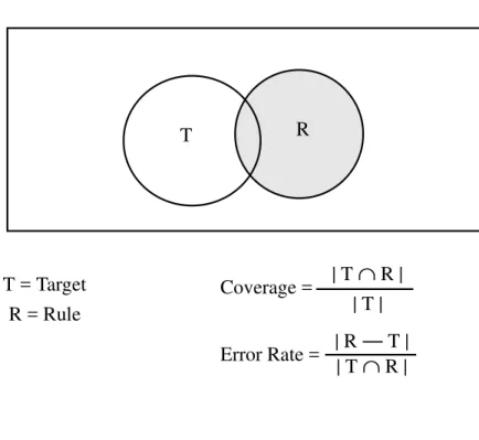
Calculation of coverage and error rate reported in each rule was done as follows: let T be the tar-get set, the set of all productions in the given batch (B) that do not meet the production specifica-tions. Let R be the rule set, the set of all productions in a given batch that satisfy the given rule. The coverage of the rule is defined as the percentage of T that is covered by R. In other words, the coverage is | T

∩

R | / | T |, where |...| represents the cardinality of a set. The error rate is the ratio of errors to successes for the rule, | R — T | / | T

∩

R |, where | R — T | is the set of productions that are in R but not in T (see Figure 6).

The analysis involved randomly splitting the data into a training and a testing set. The rules gener-ated on the training set are evalugener-ated on the testing set. In Table 3, the coverage and error rate are reported independently for the training and the testing set.

(35)

100 observations from production of parts. The production engineers normally accept or reject a product based on the postform measurements of the part. For 26 of the postform measurements there were upper and lower limits on the values of the parameters. The distance between the upper and lower limits was, in most cases, 0.007 in. For each of the 26 postform parameters, there were two possible problems: the parameters could be below the lower limit or they could be above the upper limit. Therefore, a total of 26 * 2 = 52 different classes of problems were defined. A rejected part may have several different problems, so the 52 classes of problems have substantial overlap. An alternative could have been to simply define 26 classes of problems, one for each postform measurement.

The analysis process resulted in generating decision trees similar to the tree shown in Figure 5. ________________________________________

Approximate location of Figure 5

________________________________________

Figure 5 is an example of a decision tree for one of the 52 different classes of problems. This deci-sion tree uses thresholds on the values of two preform parameters to predict whether center-kk-postform (one of the center-kk-postform parameters) will be above the upper limit. To make a prediction, one must start at the top of the tree and move down, following the branch that applies to the cur-rent part. The terminal nodes of the tree (rectangular boxes) are predictions about the postform parameters. The non-terminal nodes of the tree (elliptic boxes) may contain either preform or operation parameters.

The terminal nodes of a decision tree represent mutually exclusive classes. Since a part may have several of the 52 different possible classes of problems, one cannot use a single decision tree for

(36)

________________________________________

Rules induced from real data (especially if the data are noisy) may sometimes have a tendency to overfit the training data (Quinlan, 1986). Some rules generated from a few examples are often testing irrelevant attributes, fitting the noise in the training data. Such rules lower the accuracy of applying induction to the analysis process. This is specially true if the training set lacks the required number of examples of the target concept. Quinlan’s C4.5 algorithm (Quinlan 1993) gen-erally avoids this problem. The learning system used here makes sure that at least two positive examples and two negative examples of every target concept exist in the batch of data.

Decision tree algorithms, such as ID3, normally avoid irrelevant attributes. However, some times when a decision tree is built it may be difficult or uneconomical for users to apply all the attributes reported in each rule. It is therefore desirable to have a preference on the attributes that are selected by the induction algorithm. Two common ways of achieving this are: (i) to impose some criteria on checking the preference of attributes before reporting the rules and (ii) possibly remov-ing portions of the rule or the entire rule that is not to be contributremov-ing to the improvements of the process. This is currently done by domain experts who have sufficient knowledge about the pro-cess. However, this is one of the tasks that can be incorporated into the expert system component of the architecture (Figure 1).

5.1 Method

The main challenge to any learning system is to learn from a relatively small sample and to suc-cessfully make predictions on new cases. Here, data were analyzed in batches of approximately

(37)

________________________________________

Tables 1 and 2 show examples of some facts and rules that are included in the domain model. This approach in building the domain model allows one to update the knowledge base as learning pro-ceeds. Every time that new knowledge about the process behaviors is discovered, the relevant knowledge about the old behaviors is updated or discarded. This is discussed in Section 6.

5.0 Rule Induction

Rule induction refers to mathematical methods for analyzing sets of data consisting of both logi-cal and numerilogi-cal variables to produce decision trees or influence diagrams. The analysis process generates substantial amounts of new information and the decision trees or influence diagrams generalize this information into useful knowledge. Decision trees are special instances of the gen-eral class of disjunctive normal form (DNF) production rules. In a tree, each branch to a terminal node represents a conjunctive rule, and the set of all branches to terminal nodes for a class is the disjunction of the rules. The key characteristic of the set of rules formed by a decision tree is that they must all share the root node test. For example, in order to learn to recognize the problems associated with the center-kk-postform-high (center-kk-postform > - 0.50), IMAFO’s learning mechanism induces rules from a collection of positive and negative examples of center-kk-post-form-high. Table 3 shows examples of two rules for this subspace. Both rules in this set have p-out-act (pressure-out actual) as the first attribute (root node), i.e., the two rules share the testing of the root node.

(38)

ters. Influence diagrams offer an important complement to more traditional knowledge represen-tations, such as decision trees and tables of joint probability distributions. Influence diagrams may also be used to determine the outcome values for each action and state. In addition, influence dia-grams can provide an explicit representation of probabilistic dependence and independence in a manner accessible to both human and computer. The basic difference between an influence dia-gram and a causal model is the use of +/- signs. These signs are used in causal models to show the positive change increase or decrease between two parameters.

(39)

(1988, 1990) in which the entire knowledge base of a process is divided into three layers. The first layer contains the laws and rules that govern a process (strategy knowledge). This layer deter-mines what domain knowledge is relevant to the management of the process at any given time and what additional information is needed to solve a particular problem case. The strategy knowledge also approximates a cognitive model of heuristic classification problem solving. The second layer, in Wilkin’s approach, is descriptions of the process (domain knowledge) and consists of Mycin-like rules and simple frame knowledge. The third layer includes the transient information that may change at any instant of time (problem state knowledge). Since, in this approach, the knowl-edge base is used for an expert system, this layer is generated during execution of the expert sys-tem.

The domain model here consists of Domain Specific Knowledge and Process Knowledge. Domain Specific Knowledge includes all the information about the process (ECM), such as domain theory and laws and rules that are principles of the ECM operation, regardless of any par-ticular application. Process Knowledge is mainly made up of information that is only valid for particular applications, such as machining of airfoils with an ECM unit. Most of the process knowledge is in the from of heuristic rules which are obtained from empirical results and discov-eries made by IMAFO. This approach would simplify the knowledge base refinement process when the knowledge base of the expert system is built.

The knowledge to be included in the domain model consists of two types of causal models for the entire process and a collection of various problem-specific facts, goals, procedures, and heuristic rules. Of the two types of causal models, one type illustrates the relationships among different process parameters and the other shows the effect of different preform parameters on postform parameters. Figure 3 shows a portion of a causal model developed from the basic information of the ECM process and the relationship among different process parameters. Figure 4 shows an example of a portion of an influence diagram that was manually constructed from discoveries made by IMAFO. This diagram shows the relationship between preform and postform

(40)

parame-by electrochemical action. Figure 2 illustrates the basics of the ECM process. The main difference between ECM and traditional machining techniques is that, in ECM, metal removal from a work-piece is performed molecule by molecule. A number of parameters would affect the performance of the ECM operation. These are (i) process parameters such as feedrate, voltage, or electrolyte temperature, (ii) set-up parameters such as gap or type of fixture, and (iii) workpiece parameters, which are simple or complex geometrical properties such as thickness, bow, or warp of the work-piece before being machined.

A preliminary domain model of the process was constructed to study the ECM process and to benefit from the discoveries made by the learning system by incorporating them into the domain model. A domain model is a collection of structural and behavioral knowledge about a particular process. The structural aspect of the model represents the process components and the relation-ships among them, while the behavioral aspect describes how the status of the structure changes. Developing a domain model in a real environment is helpful because it limits the complexity of the general configuration tasks, determines the basic knowledge needed for solving configuration tasks, and also enables more efficient problem solving methods (Mittal and Frayman, 1989). Use of domain models would allow the presentation of domain knowledge in a more structured way. In addition, when process monitoring and learning are used in conjunction with expert system technology to support the planning and decision-making task of a process, the refinement of the knowledge base and control of the search for a desired solution to a problem would be faster with a well structured domain model.

(41)

3.2 Learning Mechanism

IMAFO’s learning mechanism is based on Quinlan’s ID3 algorithm (Quinlan, 1983, 1986, 1987a, 1987b). It’s main function is to analyse the information collected from a process and to search for descriptions of unsuccessful plans and operations as defined by the user. The learning mechanism builds a decision tree for each subspace (class of unsuccessful plans or operations) and prunes the tree.

3.3 Rule Generator

The rule generator converts each decision tree into a set of production rules that are reported to the users. This is done because large induced trees are sometimes difficult to understand and reporting them directly would not be useful to the planners and operators. Each rule consists of a coverage and an error rate. Planners and operators can then apply these rules to improve the per-formance of a process.

The most important features of IMAFO are (i) ability to handle a variety of data types, (ii) flexi-bility in allowing the users to define many complex attributes, (iii) conversion of decision tree into a more understandable form, (iv) efficient use of data to extract as much information as possible from data, and (v) automatic classification of events. For more details about the components of IMAFO and their functionality, see Famili and Turney (1991).

4.0 Electrochemical Milling Process

The domain of the application is the electrochemical milling operation. This is a Computer Numerical Controlled (CNC) process by which excessive metal is removed to finish the surface of a workpiece and produce products to within preset tolerances. The process involves passing cur-rent through an electrolyte (conductive liquid) in the gap between a workpiece and a suitably shaped tool. The electrolyte resolves and removes the reaction products formed on the workpiece

(42)

occur during the production, and incorporating any new knowledge that is discovered by analyz-ing data from the ECM process. In addition, simple causal models that show the relationship among different workpiece parameters are also prepared. Since the domain model is used for building an expert system for process setup and problem solving, causal models (e.g. an influence diagram) can be used for providing explanations for the decisions made by the expert system.

3.0 IMAFO

IMAFO, the core of the intelligent supervisory system, is written in Common Lisp and runs on a SUN workstation. IMAFO consists of an interface, an initialization mechanism, a learning mech-anism, and a rule generator (see Figure 1). The interface is window based, hierarchically struc-tured, and available options are displayed in smaller windows or buttons. A description of the remaining components of IMAFO follows.

3.1 Initialization Mechanism

The initialization mechanism provides a uniform structure for defining different applications for analyzing data from the execution of plans or operations (e.g. productions) from various types of industrial processes. A number of steps must be followed during initialization. These are (i) spec-ifying the format of input files, (ii) defining a measurement space, through which different sources of input are consolidated into a number of vectors in a multi-dimensional space, (iii) defining sub-spaces of measurement space (classes of problems), and (iv) controlling the use of dimensions of the measurement space that IMAFO can use for generating the concepts (rules).

(43)

For the process to be optimized, we first identified all process and workpiece parameters that were known to be related to the performance of the process and quality of the end product. These were parameters that could be (i) measured and recorded on the workpiece before the machining cess (preform parameters), (ii) measured and recorded automatically during the machining pro-cess (operation parameters), and (iii) measured and recorded on the workpiece after the machining process was completed (postform parameters). A total of 30 preform parameters, 22 process parameters, and 30 postform parameters were recorded for each production. While IMAFO used preform and operation parameters to correlate them with unacceptable workpieces, postform parameters were the basis to classify the productions into acceptable and unacceptable. The entire set of production data consisted of 1369 observations that were divided into batches of approximately 100 observations. The data were then converted to a format that was understand-able by IMAFO (list of elements, each representing the numerical or symbolic value for an attribute). To analyze each batch of data by IMAFO, an initialization file was created that con-tained information about data files, a list of parameters, and constraints of the postform parame-ters (classes of unacceptable productions).

Each batch of data was then analyzed by IMAFO and the output was recorded in separate files. IMAFO’s analysis of data consisted of some statistical information about the observations fol-lowed by rules predicting the cause of different problems. Manual interpretation of the rules was a complex task that consisted of five steps: (i) selecting useful rules, (ii) selecting commonly occur-ring parameters, (iii) selecting parameters occuroccur-ring in two or more rules, (iv) summarizing con-clusions for each class of problem, and (v) preparing suggestions to optimize process and workpiece parameters. These steps are discussed in detail in Section 5.

The knowledge generated during this phase is incorporated into the domain model of the ECM process. The objective of using a domain model is to provide a framework for structuring and documenting the knowledge about the ECM process, investigating and solving problems that may

(44)

medical, automotive, and aerospace applications. Furthermore, we discuss how decision-tree induction can help in building the domain model of this complex process and refining its knowl-edge base is discussed. Results of analyzing various experimental data from the ECM process and examples of how the results are used for process improvement are presented.

The analysis has been done using a software package called IMAFO (Intelligent MAnufacturing FOreman) developed by the authors at the Knowledge Systems Laboratory of NRC. IMAFO is the core of an intelligent supervisory system that helps industrial planners and operators to dis-cover the reasons for unsuccessful plans and operations. The structure and features of IMAFO are briefly discussed in Section 3. The ECM process is explained in Section 4. In Section 5, rule induction and the method developed to analyze the induced decision-trees are discussed. Section 6 shows how the generated rules are used to optimize the ECM process and to refine an existing knowledge base in an intelligent supervisory system. In the conclusion, direction of our research and future goals are presented.

2.0 Overview of the Approach

Although one of the main goals of artificial intelligence is to develop intelligent systems that embody all the components of intelligence, few attempts have been made to build systems that integrate multiple features, such as situation recognition, learning, and advanced reasoning. Our long term goal is to design and implement an intelligent supervisory system capable of process monitoring, situation recognition, learning, and environment representation. The system is to be used for monitoring and analyzing plans and operations in an industrial environment, explaining why they fail, and suggesting appropriate actions. Figure 1 illustrates the basic architecture of the intelligent supervisory system. The core of this system, IMAFO, has been developed and tested with simulated data (Famili and Turney, 1991). This paper describes the results of applying IMAFO for process optimization and support in knowledge refinement of a complex automated process in which metal parts are machined.

(45)

1.0 Introduction

Construction of expert systems begins with the knowledge acquisition process that has different modes. In its simplest mode, the knowledge engineer consults various textbooks and manuals and extracts additional knowledge from domain experts to build the knowledge base of the expert sys-tem. However, when the domain is a complex automated process for which a sufficient amount of domain knowledge is not available, the knowledge base can be augmented using machine learn-ing techniques. This approach would help to optimize the plannlearn-ing and decision-maklearn-ing aspect of the process and to reduce the dependency on the quality and quantity of the knowledge to be acquired from texts, manuals, and domain experts.

Machine learning is a process by which a computer can acquire new knowledge from experience (e.g. test cases) to improve the performance of a knowledge base (Michalski, 1986). A common approach to learning, when machine learning techniques are used, is decision-tree induction in which a decision tree is developed from a set of examples of test data. Decision trees normally consist of a number of nodes, each representing an attribute with different instances that are used to classify the test cases and build the tree. When decision trees are built, they are pruned and con-verted to a set of rules that can be easily understood and applied by users.

Important advantages of using machine learning in building the knowledge base of an expert sys-tem are:

• discovering new knowledge (e.g. rules) explaining the situations that would be sometimes impossible to know otherwise,

• automatically refining the knowledge base for various applications of the same domain.

This paper presents the basic idea of using decision-tree induction in process optimization of an Electrochemical Machining (ECM) operation. The ECM process is used by industries to perform the final stage of producing metal parts that require precision machining operations. Examples are

(46)

Use of Decision-Tree Induction for Process Optimization

and Knowledge Refinement of an Industrial Process

A. Famili

Knowledge Systems Laboratory Institute for Information Technology

National Research Council Canada Ottawa, Ontario, Canada

K1A 0R6 famili@ai.iit.nrc.ca

Abstract

Development of expert systems involves knowledge acquisition which can be supported by applying machine learning techniques. This paper presents the basic idea of using decision-tree induction in process optimization and development of the domain model of electrochemical machining (ECM). It further discusses how decision-tree induction is used to build and refine the knowledge base of the process.

The idea of developing an intelligent supervisory system with a learning component (IMAFO, Intelligent MAnufacturing FOreman) that is already implemented, is briefly introduced. The results of applying IMAFO for analyzing data form the ECM process are presented. How the domain model of the process (electrochemical machining) is built from the initial known informa-tion and how the results of decision-tree inducinforma-tion can be used to optimize the model of the pro-cess and further refine the knowledge base are shown. Two examples are given to demonstrate how new rules (to be included in the knowledge base of an expert system) are generated from the rules induced by IMAFO. The procedure to refine these types of rules is also explained.

(47)

List of Tables

1. Examples of some facts that are included in the domain model 2. Examples of rules that are included in the domain model 3. Examples of rules generated for centr-kk-postform high 4. (a, b, and c) Examples of rule reduction

5. An example of a recommendation 6. (a and b) Examples of rule refinement 7. (a and b) Examples of induced rules 8. (a and b) Examples of rule refinement

(48)

List of Figures

1. The architecture of the intelligent supervisory system 2. The ECM process

3. A portion of the causal model of the ECM process parameters

4. A portion of the causal model with the relationships between preform and postform parameters 5. An example of a decision tree

(49)

Table 8 (a and b). Examples of rule refinement Rule

If

Then

(a) Rule

If

or

Center-kk-preform is less than -0.54505 Then

(50)

Table 7 (a and b). Examples of induced rules

(a) rule 1

centr-kk-0 is less than -0.54480 coverage 92.0% (train) 92.0% (test) error rate 2.2% (train) 4.3% (test) rule 1

centr-kk-0 is less than -0.54505 coverage 82.4% (train) 62.5% (test) error rate 0.0% (train) 0.0% (test)

(51)

Table 6 (a and b). Examples of rule refinement

Rule If

Pressure-in-actual should be more than 202 (a)

Rule If

Pressure-in-actual should be more than 203 (b)

(52)

Table 5: An Example of a Recommendation

variable influences suggestion

(53)

Table 4- Continued (a, b, and c). Examples of rule reduction

subspace mid-dd-hi: rule 1

plat-in-conc-0 is more than -42.38720 mid-dd-0 is less than 0.13420

rule 1

chord-ff-0 is less than 1.03595 sum-chord-0 is more than 3.09970 mid-dd-0 is more than 0.13770

plat-out-conv-le-0 is more than 0.01015 coverage 20.0% (train) 11.1% (test) error rate 0.0% (train) 0.0% (test)

(54)

Table 4 (a, b, and c). Examples of rule reduction

plat-in-conv-0 is less than -42.87760 le-dd-0 is more than 0.08855

rule 1

a )

subspace te-ff-lo: rule 1

p-in-act is less than 202.26500 shuttle-num is not 5

warp-kk-0 is more than -0.79905 coverage 50.0% (train) 20.0% (test) error rate 0.0% (train) 0.0% (test)

rule 1

p-in-act is less than 203.50000

(55)

Table 3. Examples of rules generated for the centr-kk-postform high

subspace centr-kk-hi: rule 1

p-out-act is less than 73.41000 coverage 94.7% (train) 73.7% (test) error rate 0.0% (train) 0.0% (test)

rule 2

p-out-act is more than 73.41000 le-dd-0 is more than 0.08370

coverage 5.3% (train) 21.1% (test) error rate 0.0% (train) 0.0% (test) combined rules

(56)

Table 2. Examples of rules that are included in the domain model Rule If Gas-level > x1 and Electrolyte-temp > x2 Then Electrolyte-resitivity Constant Rule If Center-kk is high or Center-kk is low Then Center-kk-perform should be > -0.54505 Center-kk-preform should be < -0.52525

(57)

Fact (center-kk-postform high -0.50) and (center-kk-postform low -0.52) Fact (gap-voltage on-time 18) and (gap-voltage off-time 17.5)

(58)

T = Target R = Rule Coverage = Error Rate = | T

∩

R | | T | | R — T | | T

∩

R | T R

(59)

Figure 5. An example of a decision tree False

False True

center-kk-postform will be above the upper limit

center-kk-postform will be below the upper limit center-kk-postform will

be above the upper limit

le-dd-preform > 0.0837 True

(60)

Figure 4. A portion of the causal model with the relationships between pre-form and postpre-form parameters

le-dd-0 centr-dd-0 centr-kk-0 plat-out-conv-le-0

le-dd-hi centr-kk-lo centr-dd-lo warp-kk-lo mid-dd-hi centr-kk-hi

le-dd-lo

preform parameters

postform parameters

(61)

Figure 3. A portion of the causal model of the ECM process parameters feed rate voltage inlet

pressure

inlet temperature concentration of

electrolyte

process parameters _{set up parameters} current

density gap flow rate

electrolyte velocity electrolyte conductivity operating temperature gas portion of electrolyte

positive change increase positive change decrease

(62)

(63)

Figure 1. The architecture of the intelligent supervisory system

IMAFO

Expert System

Reasons for Failed Plans

Industrial Process

Execute Succeeded Plan Operators/ Engineers

- Analysis of Process Information - Advice to Operators/Engineers Inference Mechanism Advice Generator Knowledge Base Domain Specific Knowledge Planning Information Execute Succeeded Plan Execute Plan Process Monitoring Module Data Conversion Module Data Collection Schedule Learning

Mechanism Initialization_Mechanism

User

Interface _GeneratorRule

Process Knowledge User Interface Setup Information Failed • • • Planning & Execution Information

(64)

Biography

A. (Fazel) Famili is a Senior Research Officer at the Knowledge Systems Laboratory of the Insti-tute for Information Technology of the National Research Council of Canada. Dr. Famili received his M.S. from The Ohio State University and his Ph.D. from Michigan State University. Prior to joining NRC (in 1984), he worked for industry for three years. His current research focuses on Machine Learning, Expert Systems, Applications of A.I. in Manufacturing, and Intelligent Super-visory Systems. He has published or has been the co-author of several articles in these areas and edited (with Steve Kim and Dana Nau) the AI Applications in Manufacturing book that was pub-lished by MIT/AAAI press in 1992. He is also in the editorial board of two scientific journals and is a member of AAAI.

(65)

Turney, P. and Famili, A. 1992. Analysis of induced decision trees for industrial process optimiza-tion, Proceedings of the 6th International Conference on Systems Research, Informatics and Cybernetics, pp. 19-24.

Widmer, G., Horn W., and Nagele, B. 1992. Automatic Knowledge Base Refinement: Learning from Examples and Deep Knowledge in Rheumatology, Report No. TR-92-16, Austrian Research Institute for Artificial Intelligence.

Wilkins, D.C. 1988. Knowledge Base Refinement using apprenticeship learning techniques, Sev-enth National Conference on Artificial Intelligence, Vol. I, pp. 646-651, Morgan Kaufmann Los-Altos, California.

Wilkins, D.C. 1990. Knowledge Base Refinement as Improving an Incorrect and Incomplete Domain Theory, Report No. UIUCDS-R-90-1585, University of Illinois, Urbana, IL.

Wylie, R.H. and Kamel, M. 1992. Model-based knowledge organization: a framework for con-structing high-level control systems, Expert Systems with Applications, 4(3); 285-296.

(66)