Measurement of flow field and wall temperature distribution in a scraped heat exchanger crystallizer

HAL Id: hal-00193852

https://hal.archives-ouvertes.fr/hal-00193852v3

HAL is a multi-disciplinary open access archive for the deposit and dissemination of sci-entific research documents, whether they are pub-lished or not. The documents may come from teaching and research institutions in France or abroad, or from public or private research centers.

L’archive ouverte pluridisciplinaire HAL, est destinée au dépôt et à la diffusion de documents scientifiques de niveau recherche, publiés ou non, émanant des établissements d’enseignement et de recherche français ou étrangers, des laboratoires publics ou privés.

distribution in a scraped heat exchanger crystallizer

Marcos Rodriguez, Florent Ravelet, Rene Delfos, Geert-Jan Witkamp

To cite this version:

Marcos Rodriguez, Florent Ravelet, Rene Delfos, Geert-Jan Witkamp. Measurement of flow field and wall temperature distribution in a scraped heat exchanger crystallizer. 5th European Thermal-Sciences Conference, May 2008, eindhoven, Netherlands. pp.hex_2. �hal-00193852v3�

MEASUREMENT OF FLOW FIELD AND

WALL TEMPERATURE DISTRIBUTION IN

A SCRAPED HEAT EXCHANGER CRYSTALLIZER

M. Rodriguez Pascual

, F. Ravelet

, R. Delfos

, G.J. Witkamp

1

Process & Energy Dept. Delft University of Technology, the Netherlands

2

Laboratory for Aero and Hydrodynamics, Delft University of Technology, the Netherlands

3

lnstitut de Mécanique des Fluides de Toulouse, France

Abstract

During crystallization the control and effective distribution of heat transfer from the solution to the heat exchanger (HE) plays an important role. Inhomogeneity in temperature on the HE-surface limits the production capacity and increases the tendency of an isolating scale layer formation. To avoid scaling, scraper blades on the HE are commonly used.

In a typical axi-symmetric geometry the scale layer formation was investigated. We studied the influence of the flow field on the actual heat transfer distribution 1) by directly measuring the surface temperature field of the HE using LCT and 2) by measuring the flow field inside the crystallizer using 3C-PIV.

From Liquid Crystal Thermometry, we can clearly see that, except for the centre region, near the inside the heat transfer is considerable better than near the outside. Stereoscopic PIV velocity measurements reveal that the central region of the crystallizer is in solid body rotation; in the outer parts there is a strong secondary flow, where crystallizer solution descends onto the HE-surface, causing a high heat transfer; near the outer wall the solution rises again having a small heat transfer. We conclude that the present design of the stirrer / scraper system in the crystallizer provides sufficient secondary flow to keep the system mixed. However, near the outer wall and near the shaft the heat transfer is considerably lower than average. This is also the zone where during Eutectic Freeze Crystallization experiments the first not-removed ice-scaling layer is observed. This is thus not due to a limited scraping function of the scraper, but due to the HE getting the lowest temperature, hence the highest sub-cooling.

1 Introduction

Several crystallization processes consist of liquid solutions that by the action of heat exchangers are brought into supersaturated regions where crystals will form. In industrial continuous processes, where solution is constantly fed into the crystallizer, control and stability of the bulk solution temperature is mandatory. For this reason a degree of turbulent flow in the crystallizers is necessary to achieve good mixing of the whole solution. The heat transfer rates are directly responsible for the production rates. The residence times of the solution in the crystallizer will determine size and quality of the crystals.

To obtain the desired supersaturation the solution is cooled down (as in Eutectic Freeze crystallization) or heated up (as in Evaporative Crystallization). This action is done by Heat Exchangers (HE) in direct contact with the solution. Near the HE surface exists a thermal boundary layer that depends on the crystallizer flow characteristics. Here the supersaturation is higher that in the bulk solution. Because of the higher supersaturation on the HE surface the nucleation and growth rates of the crystals are faster than in the bulk solution. This situation is responsible for the formation of a scaling layer of crystals on the HE surface. As a consequence produces a decrease of heat transfer, affecting the stability of the crystallization process. To avoid this scale layer formation, it is common to use mechanical actions, such as scraping.

The scraping efficiency is directly proportional to the temperature difference between the bulk solution and the heat exchanger surface temperature [Vaessen (2002) and Pronk (2005)]. Depending on our solution and the characteristics of our mechanical scraping action (velocity, shapes and applied forces), we will have a maximum temperature difference between the solution and the heat exchanger surface where scaling will appear. In order to achieve the desired production rate and avoid the scaling layer problem we will have to apply the consequent scraping characteristics. For these reasons the heat exchanger surface temperature has to be as uniform as possible to control the unwanted scaling layer.

2 Ice scaling Experiments

2.1 Setup

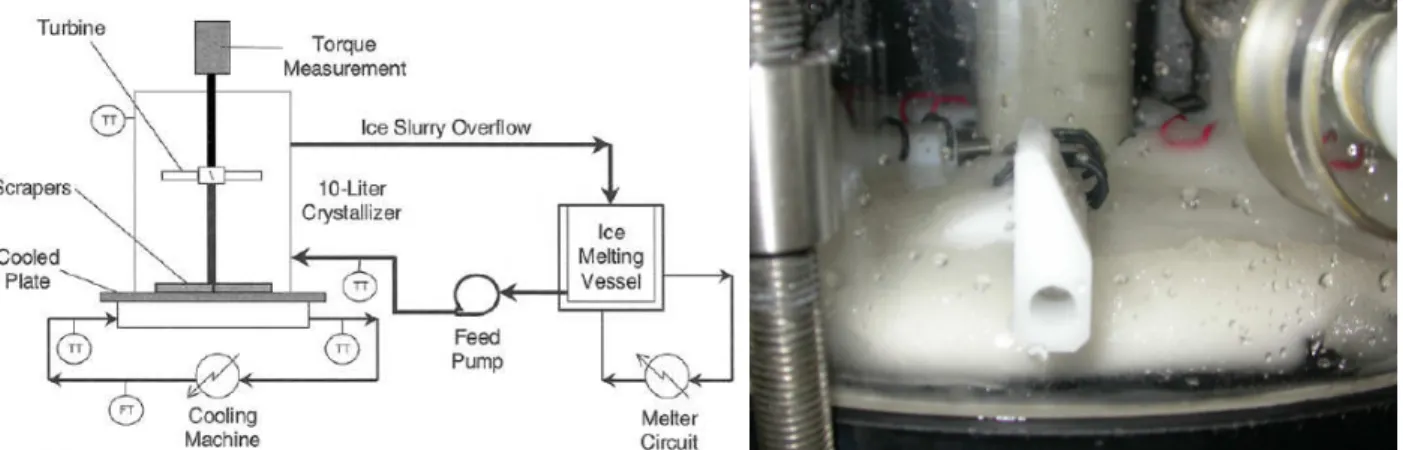
The experimental set-up for ice-scaling research (Ice Scaling Crystallizer, ISC) consists of a 10-liter scraped surface crystallizer as shown in Figure 1. The crystallizer has a 1 mm stainless steel bottom plate with a heat transfer area of 0.031 m2, which is scraped by four rotating Teflon scraper blades

that are driven by a vertical shaft. Halfway this shaft, a turbine mixer is installed to keep the slurry homogenously mixed. The bottom plate is the topside of a Heat Exchanger (HE), which is cooled by a 50 wt% potassium formate solution (‘Freezium’). The coolant follows a spiral channel through the HE. Height & width of the channel measure 5 & 17 mm, respectively. The coolant flow rate is 1000 l/h, resulting in a channel velocity of over 3 m/s, guaranteeing turbulent channel flow. The HE inlet temperature is controlled within 0.1 K by a cooling machine.

The crystallizer overflows to an ice-melting vessel were the produced ice crystals are molten and from which aqueous solution is pumped back to the crystallizer, such facilitating stationary flow conditions. To minimise heat leaks to the ambient, the experimental system was thermally insulated wherever appropriate besides some selected parts required for (visual) observation.

Temperature of the coolant (at inlet and outlet), the crystallizer liquid (near top and bottom of the vessel) and the feed flow were measured with ASL F250 precision thermometer connected to PT-100 temperature sensors with an accuracy of ±0.01 °C. The pressure of the coolant in the HE channel was measured at inlet and outlet by two analogue pressure sensors with an accuracy of

±0.001 bar. The flow rate of feed solution and coolant were measured with two electro-magnetic flowmeters with an accuracy of ±1l/h. The five temperatures, the two pressures and the two flow rates were collected every 1 second in a computer using the LabView data acquisition program.

Figure 1. Scheme for performing continuous crystallising experiments.

Figure 2. The bad local heat transfer distribution on the HE surface translates into high

temperature differences through the HE surface. As observed during ice scaling experiments in the ISC lower temperatures where found in the centre of the HE and in the outer area, forming two rings with difference on temperature compare with the middle ring higher than 4 oC. Due to this difference on temperature the nucleation and crystal growth are higher in the centre and in the outer ring and is this zones where ice scaling starts.

This same behaviour was observed in the CDCC ending with a damaged outer scraper because of the impossibility to remove the thick ice layer formed in this area.

2.2 Observations

During all experiments in the ISC, the temperature of the crystallizer liquid constant, i.e. at the freezing temperature of the water, or at the eutectic temperature for a salt water system. With this system, we have run experiments in which we gradually increase the heat flux through the HE by gradually lowering the HE temperature. Doing so, we find that ice scaling (i.e. the formation of ice that is not removed by the scraper blades) starts in two distinct areas of the HE surface: 1) near the centre of the crystallizer and 2) close to the outside wall. The net effect is the formation of two rings of ice. When one keeps the process going anyway, the scrapers gradually get lifted up, and the function of the scrapers quickly deteriorates. In experiments in the ‘CDCC’ crystallizer (a scaled-up version of the ‘ISC’, Genceli (2005)), exactly the same behaviour is observed. As we can see in Figure 2, continuation of the process ended with damage to the outer scraper.

Possible explanations for this reproducible behaviour were as follows:

1) The scrapers function better in the middle section. This argument was discarded, because also when we scraped with arms of three independent scraper sections (each with their own spring loading) we observed exactly the same behaviour.

2) Influence of the feed flow inlet. The feed flow inlet is always slightly warmer than the crystallizer fluid. We have visualized the flow pattern by injecting a blue dye into the feed flow. There we observed that, when entering the crystallizer, the dye is first transported upwards, then mixed in the top section, before it finally descends into the lower section where it contacts the HE surface. By that time, it has mixed well, and cooled down sufficiently.

3) Possibly the local heat transfer varies over the plate. Since we could cross out the first two mechanisms, we have done a more elaborate study on the latter process.

We have done in-situ measurements of the heat exchanger surface temperature distribution, and consequently the local heat transfer distribution, which is described in section 3. Also, we have done quantitative flow measurements, which are described in section 4. In Section 5 we will combine and discuss the results, and consider the consequences.

3 Heat Exchanger Surface Temperature Measurements

3.1 Experimental Setup

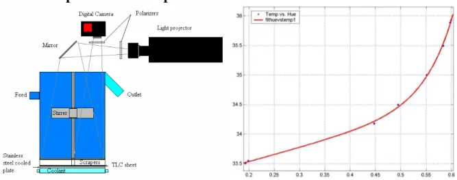
Figure 3. Sketch for the set-up for surface temperature measurement.

The set-up for measuring the HE surface temperature is shown in Figure 3. This temperature was measured using an adhesive thermochromatic liquid crystal sheet (TLC, Hallcrest R34C1W) glued directly onto the HE-surface. The TLC changes colour with temperature, with a working range between 34-35 °C (provider-specified). The TLC-sheet is illuminated using a slide projector with ‘white light’ (320 W halogen lamp, colour temperature 3400 K). Its light is passed through a linear polarising filter, then projected via a mirror onto the bottom of the tank under an angle of incidence of about 15° with the vertical (‘lighting angle’). The TLC-sheet surface was observed from above under an angle of 15° as well (‘viewing angle’) through a second polarizer using a digital photo camera (Canon Powershot S2 IS). The two polarizers suppress unwanted reflections of the illuminating light, resulting in more saturated TLC-reflected colours. Colour TLC surface photographic images (jpeg-compressed, 2592*1944 px) were recorded and transferred to a PC every 2 seconds, on which further image processing was done using MatLab, v. 6.0.

Calibration of the TLC-colours was done in situ, in the same manner as described in Delfos & Lagerwaard (2003). In short: during a gradual heat-up and cool-down procedure when the temperature on top the TLC and the temperature of the coolant readings were stable at the same value within 0.01 oC, an image was selected for the calibration curve. The Red-Green-Blue (RGB) data was mapped to Hue-Saturation-Intensity (HSI) data using MatLab's rgb2hsv function. Based on the Hue values H, we obtain a one-to-one relationship for T vs. H. The useful part of the resulting calibration curve runs is in the range 33.5 °C < T < 36 °C (Figure 4), as in Delfos & Lagerwaard (2003) and was shown to depend only little on illumination intensity with an accuracy of ±0.03 °C.

To avoid hysteresis effects of the TLC due to the working range we decide to study the HE surface temperature in an inverted experiment, where instead of cooling the solution we heated up to avoid exposing the TLC sheet to high temperatures. This means: the solution is maintained at a temperature of some 32 oC; it is heated through the HE with ‘coolant’ of 42 oC; the feed flow is about 28 oC. After a stationary situation was obtained (monitored using thermometers), imaging was started. In Figure 4 we see a typical picture of (half of) the TLC sheet on the heat exchanger as measured halfway during this time interval. The shiny part is one of the steel arms that hold the scraper. This result immediately shows that, even though at first glance the process as a whole is stationary, that there is a strongly non-uniform temperature distribution on the HE surface.

3.2 Results - integral heat transfer

To get a view on the energy balance of the system, we applied the following steps. The total heat flux through the heat exchanger surface into the crystallizer, Q&_HE, is directly found from the integral energy balance:

(

)

(

)

HE cool cool V cool loss

Q& = φ ⋅ρ ⋅ c ⋅∆T − ∆p −Q& , (1)

where φcool, ρcool and cV are the flow rate, density and its specific heat of the coolant; ∆Tcool and ∆p

its temperature and pressure drop in the coolant channel, and Q&_loss the heat flux to the surroundings. The latter was determined experimentally earlier for this HE (Pronk et al (2006)), and is here estimated as 1.5 W/K. For the experimental conditions as above, we have an estimated heating of the crystallizer solution of 220 W. For instationary heating as in our case, this net heat flux is absorbed by the solution and the feed liquid:

HE feed sol V cryst

Q& =Q& +Vol⋅ρ ⋅ ⋅c dT dt, (2)

where Q&_feed is calculated the same as for the HE flux, and the solution temperature rise, dTcryst /dt is

obtained from the measurements as 0.0017 oC/s.

This give a Q&_feed of 120 W average during the measurement time, which means a total heat taken by the solution of 100 W and an increase of 0.57 oC, whereas the experiment has a measured

increase of 0.4 oC. Taking into account the limited accuracies, we consider this a sufficient approximation.

3.3 Results - local heat transfer

In the previous we have considered the total heat transfer from coolant to crystallizer solution. Since we have observed that the HE surface temperature is much dependent on position, we need to search for the local surface heat flux, q& and local heat transfer coefficient h. Since we observe that the TLC colour pattern on the HE surface (so presumably also the temperature) is more or less axis symmetric, we assume further that all profiles are functions of the distance to the centre, r, only. Then we can write in general the local relation between q& and h (Mills 1999):

( ) ( )

(

)

h r =q r& T −T (3)

where T_cool is the average temperature of the coolant, and the solution temperature Tsol already is

assumed to be constant throughout the crystallizer.

The heat transfer coefficient for the system, h is found by adding up the individual heat resistances:

) ( / 1 / / / 1 ) ( /

1 h r = h_cool +d_plate λ_plate+d_TLC λ_TLC+ h_cryst r (4)

Here the conductive heat transfer coefficients for the stainless steel plate and the TLC layer are 15*103 W/m2.K and 1.2*103 W/m2.K, respectively. To find the convective heat transfer coefficients at the coolant channel side, hcool, is more complicated: For a flowing liquid, it is given by

.

cool cool cool

h =Nu λ d, with d the hydraulic diameter of the duct, which is 7.7 mm. The Nusselt number Nu is of the form as for turbulent duct flow (Mills, 1999):

0.8 0.3

Nu=0.024 Re⋅ ⋅Pr (5)

A result found previously for turbulent flow in our cooling channel (Pronk 2006) is about twice as large due to the curvature of the channel improving the heat transport in the channel:

0.699 0.33

Nu=0.0507 Re⋅ ⋅Pr (6)

For our typical process conditions, we find Nu = 42 hence hcool = 2800 W/m2.K.

Now with the three known heat resistances (hknown = hsteel+cool+TLC), we can calculate the local heat transfer coefficient between crystallizer and HE surface based on the temperature difference between solution (Tsol) and coolant (Tcool), and the calculated surface temperature (Tsurf) from the direct TLC Temperature values under the polyester sheet (Temp[oC] in Figure 6) as follows:

) /(

)

( surf cool sol surf known

cryst h T T T T

h = ⋅ − − (7)

To get the numerical values, we process the TLC images as described. Visually it looks as below: From the photographic image of the TLC-surface we cut out the area in between scrapers (Figure 5a), we convert the RGB values into Hue values (false colours, Figure 5b), and with the calibration curve into temperature (Figure 5c).

Figure 5a. Cut area in between scrapers of the HE surface. Figure 5b. Converted into Hue values. Figure 5c. Via the calibration curve converted into temperatures.

As expected, the heat exchanger surface temperature is far from uniform: with a temperature difference between coolant and solution of just 10 oC, the HE surface temperature varies with

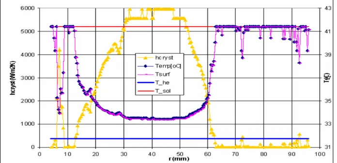
differences of more than 4 oC, and in fact even outside the working range of the TLC! We converted these data into a radial profile of the temperature distribution T(r), as is shown in Figure 6, together with the related local heat transfer coefficient, hcryst(r).

Figure 6. Radial distribution of temperature T(r) and convective heat transfer coefficient hcryst(r) on

HE surface (between scrapers). Note: temperatures above 36oC are approximate (being outside the proper calibration range), as commented before.

We now indeed clearly see near the crystallizer centre and close to the outside that the heat transfer between HE and solution, hcryst(r), is lower than that somewhat halfway the radius by a factor of at

least five. This observation of temperature and heat transfer distribution in our opinion completely explains the observation of ice scaling in the ISC experiments: in regions where the heat transfer is low, the HE surface temperature falls to lower values; thereby it increases the supersaturation of the solution, hence in these regions the nucleation will be much stronger and so the tendency of scaling. The remaining question is however the reason why hcryst varies so much over the HE plate. For this,

we will investigate the flow pattern and the turbulence present above the HE plate.

4 Stereoscopic PIV Flow Measurements

To investigate the origin of the so much varying local heat transfer coefficient, we decided to try to get more insight into the flow field and the turbulence distribution inside the crystallizer. To do so, part of the field was investigated using Stereoscopic Particle Image Velocimetry, (3C-PIV). A general description of 3C-PIV, and methods to set it up can be found in Raffel et al. (1998); some specific details of our 3C-PIV set-up in Ravelet et al. (2007). The set-up is summarised below and sketched in Figure 7.

4.1 Experimental Setup

The shaft with scraper and stirrer was taken from the original 200 mm ID geometry to a slightly larger glass cylinder of 240 mm ID, which was well aligned in the two-camera stereoscopic PIV set-up of Ravelet et al. (2007). With the

vertical-radial light laser light sheet we were able _{Figure 7. Sketch of set-up for PIV measurements.} with a PIV calibration grid-image inside/

to capture double-frame PIV images from two different projections of the particle motion. The 3D calibration, the laser and camera timing and the PIV image processing were all done using Davis 7.1-7.2 (www.Lavision.de).

The measuring area measures height 45 mm and width 80 mm, starting just above the scraper and at the outer wall, all as indicated in figure 9.

4.2 Results

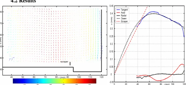
Figure 8a Average velocity field Note: the radial and tangential components are depicted as vectors, the tangential component in false colours. Figure 8b. Radial profiles of average velocity. From 500 instantaneous flow fields we obtained the average velocities and all six Reynolds stresses. Here we only consider the average velocity field and its role in the heat transfer.

The average flow field is shown in figure 8a. Also, since the flow varies only little with height, we can obtain the axially averaged radial profiles, as shown in figure 8b. The biggest velocity component is the tangential velocity, while it is forced directly by the rotating aerodynamically bluff scraper arms, and friction with the smooth outer wall and the free surface top is small. We can observe, besides a thin underresolved boundary layer at the outer wall, three distinct regions in the profile:

1) Up to a radius of roughly 50 mm, the tangential liquid velocity (blue) matches that of the scraper-stirrer shaft (dotted red). Even though data for most of this inner part is failing, it only seems realistic that this whole region, the ‘core’, is in solid-body rotation with the scraper-stirrer shaft, and there is no centrifugal or axial forcing at all; the latter is reflected as well in the small axial velocity.

2) In the annulus around the core (beyond 60 mm), the velocity decreases again, and in this region the interesting transport processes take place. The axial profile shows a strong secondary flow; near the outer wall the fluid is flowing upwards, with a magnitude as much as 15% of the tangential velocity. This strong secondary flow component driven by the rotating scraper arms, which near the bottom transport fluid outward by centrifugal forcing. Arriving at the outer wall, this flow is deflected upward as we measure it. By continuity, the fluid has to flow somewhere radially inward and then downward; here we see a maximum downward flow occurring at 80 mm from the centre. When moving radially inward or outward, the flow tends to conserve its angular momentum (Batchelor 1967); in a frictionless flow the result would be a potential vortex. As a simplified physical model to the flow, we fitted the measured tangential velocity profile with the Oseen vortex solution (Batchelor, 1967), which gradually transits from a solid-body rotation inside region to a free vortex flow outside region, as shown in figure 10b. Here we can see that in our case the picture matches qualitatively, but that the transition between the two regions is more abrupt than in the model.

The measured flow field completely supports the picture obtained from the heat transfer distribution on the HE-surface: in the core, the heat transfer is low because of the absence of a mean flow. In the annulus, there is the secondary flow, which causes much better heat transport. Locally, the heat transfer is much increased where the solution descends onto the HE-surface; the boundary layer is thinned here by the stagnation flow. In contrast, the local heat transfer is reduced where the fluid temperature has adapted to the boundary temperature and ascends. This picture of heat transfer is much similar to that measured in turbulent Benard convection, where underneath stgantion regions the heat transfer is enhanced and underneath rising plumes reduced (Delfos & Lagerwaard, (2003), and Petracci et al. (2006)).

5 Conclusions

During experiments of Eutectic Freeze Crystallization we observed that ice scaling was formed in specific areas on the heat exchanger. Because the driving force for ice scaling is the local supersaturation, and this is related to the solution temperature, we measured the temperature and heat transfer on the HE-surface.

The temperature results showed that indeed the temperature on the HE-surface was not uniform having temperature differences bigger than 4 oC, a difference more than sufficient to explain the local variation in scaling tendency. The temperature difference could directly be related to a variation in the local heat transfer coefficient over the HE-surface.

Stereoscopic PIV measurements were carried out, which showed that the secondary fluid flow in this crystallizer geometry is responsible for the inhomogeneous heat transfer distribution.

When designing cooling crystallizers and heat exchanger geometries, it is important to take flow-induced inhomogeneity in heat trasnfer into account, while this forms a strong limitation in the crystallizer performance.

References

Batchelor, G.K.(1967) An Introduction to Fluid Dynamics. Cambridge University Press.

Delfos, R. and Lagerwaard, R., (2003) Influence of large scale flow structures on convection at moderate Rayleigh numbers, Eurotherm 74, Eindhoven, March 23-26

Mills, A.F., Basic Heat and Mass Transfer (2nd Edition), Prentice-Hall, 1995

Genceli, F.E., Gaertner, R. and Witkamp, G.J., (2005) Eutectic freeze crystallization of a 2nd generation cooled disk column crystallizer for MgSO4-H2O system. Journal of Crystal Growth , 275(1-2), pp. 1369-72.

Petracci, A., Delfos, R. and Westerweel, J., (2006) Combined PIV/LIF measurements in a Rayleigh-Bénard convection cel”. 13th Int. Symp on Appl. Laser Techniques to Fluid Mechanics, Lisbon, Portugal, June 26 – 29

Pronk, P., Infante-Ferreira, C.A. and Witkamp, G.J. (2005), Ice scaling prevention with a fluidized bed heat exchanger. Proc. 16th Int. Symp. on Industrial Crystallization. pp. 1141-46

Pronk, P., Infante-Ferreira, C.A., Rodriguez Pascual, M. and Witkamp, G.J., (2005) Maximum temperature difference without ice-scaling in scraped surface crystallizers during eutectic freeze crystallization Proc. 16th Int. Symp. on Industrial Crystallization. pp. 1141-46

Pronk, P. (2006) Fluidized Bed Heat Exchangers to Prevent Fouling in Ice Slurry Systems and Industrial Crystallizers, Ph.D.-thesis, Delft University of Technology.

Raffel, M., Willert, C. and Kompenhans, J., (1998) Particle Image Velocimetry, Springer.

Ravelet, F., Delfos, R. and Westerweel, J.,(2007)Experimental studies of liquid liquid dispersion in a turbulent shear flow, paper 145 for TSFP-5, Munich, August 27-29

Vaessen, R.J.C., Himawan, C. and Witkamp, G.J., (2002), Scale formation of ice from electrolyte solutions on a scraped surface heat exchanger plate. Journal of Crystal Growth, 237-239 (Pt.3), pp. 2172-77