Publisher’s version / Version de l'éditeur:
Journal of Membrane Science, 124, 1997
READ THESE TERMS AND CONDITIONS CAREFULLY BEFORE USING THIS WEBSITE. https://nrc-publications.canada.ca/eng/copyright
Vous avez des questions? Nous pouvons vous aider. Pour communiquer directement avec un auteur, consultez la première page de la revue dans laquelle son article a été publié afin de trouver ses coordonnées. Si vous n’arrivez pas à les repérer, communiquez avec nous à [email protected].
Questions? Contact the NRC Publications Archive team at
[email protected]. If you wish to email the authors directly, please see the first page of the publication for their contact information.
NRC Publications Archive
Archives des publications du CNRC
This publication could be one of several versions: author’s original, accepted manuscript or the publisher’s version. / La version de cette publication peut être l’une des suivantes : la version prépublication de l’auteur, la version acceptée du manuscrit ou la version de l’éditeur.
Access and use of this website and the material on it are subject to the Terms and Conditions set forth at
CFD-assisted thin channel membrane characterization module design
Darcovich, Kenneth; Dal-Cin, M. M.; Ballèvre, S.; Wavelet, J-P.
https://publications-cnrc.canada.ca/fra/droits
L’accès à ce site Web et l’utilisation de son contenu sont assujettis aux conditions présentées dans le site LISEZ CES CONDITIONS ATTENTIVEMENT AVANT D’UTILISER CE SITE WEB.
NRC Publications Record / Notice d'Archives des publications de CNRC:
https://nrc-publications.canada.ca/eng/view/object/?id=ab82422c-6c40-4b42-ae58-fa3678543c45
https://publications-cnrc.canada.ca/fra/voir/objet/?id=ab82422c-6c40-4b42-ae58-fa3678543c45
journal of
M E M B R A N E S C I E N C E
ELSEVIER
Journal of Membrane Science 124 (1997) 181-193CFD-assisted thin channel membrane characterization module
design 1
K. D a r c o v i c h a,* M . M . D a l - C i n
a 9S. B a l l ~ v r e b j._p. W a v e l e t b
9a Institute f o r Chemical Process and Environmental Technology, National Research Council of Canada, Ottawa, Ont., K I A OR6, Canada b Institut Catholique d'Arts et M~tiers, Rue Auber 6, 59046 Lille Cedex, France
Received 23 January 1996; revised 19 June 1996; accepted 19 June 1996
Abstract
This project involved the design of a thin channel cross-flow module for the characterization of flat ceramic membranes. A primary objective of this work was to ensure that the flow characteristics over the permeating area were uniform.
To house these membranes, a thin channel module with a long rectangular base was envisioned. The module feed is supplied by a multi-inlet tube-type plenum meant to provide a uniform flow distribution through pressure equilibration attained in its volume.
The design criteria for the module were minimization of both the flow non-uniformity and the pressure drop across the permeating area which was a central rectangular portion of a larger slab-style cell. The flow non-uniformity was taken as the normalized standard deviation of the velocity field above the permeating area. The pressure drops considered were those across the inlet plenum and across the permeating area normalized with respect to the outlet pressure.
The computational fluid dynamics (CFD) scheme which calculated the above module characteristics was a k - e based turbulent transport model which used the finite difference method.
Design variables considered were: the plenum diameter, module width, height and length, and the diameters, distribution and number of the inlets on the plenum. The distribution of the inlet diameters was determined by two variables: either a linear or parabolic profile of variable slope and model coefficient. The operating variables were the cross-flow velocity and the plenum inlet pressure.
A two-level factorial design was used to screen the design variables. A refined three-level factorial design was used with a reduced set of design variables to optimize the module and study the response surface.
The final module design parameters were chosen such that the design criteria of flow uniformity and low pressure drop were met under a preset range of operating conditions. The local gradients of the response surface were used to verify that the design criteria were not overly sensitive to the selected module design parameters.
Keywords: Cross-flow module; Computational fluid dynamics (CFD); Factorial experimental design; Flow uniformity; Flow distributor
* Corresponding author. Fax: + 1 (613) 9412529. i NRCC No. 37618.
1. Introduction
M e m b r a n e characterization can b e a c h i e v e d m o r e readily in a m o d u l e d e s i g n e d e x p r e s s l y for this pur- pose. M a n y p r e s e n t - d a y test cells are c o n s t r u c t e d such that they create irregular and c o n f o u n d i n g hy-
0376-7388/97/$17.00 Copyright © 1997 Published by Elsevier Science B.V. All rights reserved.
182 K. Darcovich et al. / Journal o f Membrane Science 124 (1997) 181-193
drodynamic conditions. The aim of the present study is to design a membrane module for research pur- poses with uniform flow characteristics over the permeating area. A well designed and uniform flow will allow a more accurate determination of mass- transfer properties at the membrane surface in cross- flow filtration. Cross-flow filtration is increasingly employed in many industrial separation processes, such as the harvesting of bioreaction products from fermentation broths, the recovery of metal precipi- tates from waste water, and the removal of fine particles from liquids in electronics industries.
The need for this new module arose in the context of a project to develop and assess ceramic mem- branes. These ceramic membranes are to be fabri- cated by a colloidal destabilization technique so that a flat membrane will result. Presently, in our labora- tories there are disc-type cells for testing small circu- lar polymeric membranes. These existing cells would not be easily adapted to hold ceramic membranes, so it was decided to design a next-generation test mod- ule to supersede the present test cells in their ability to provide data for membrane characterization.
Cross-flow filtration is a process for filtering and concentrating a multi-component feed stock, in which the feed flows parallel to the filtration surface. With this operating configuration any solid or liquid reten- tate which might be formed on the membrane sur- face is swept away. Typically, a liquid feed at ele- vated pressure flows through a channel whose walls are permeable.
Previous work on cross-flow filtration has shown that cross-flow velocity is the key control operating factor for polarized cake or gel formation, where a faster cross-flow velocity usually gives a higher fil- tration rate [1].
Examples can be found of cross-flow modules designed without inlet pressure equilibration. Such resultant flow characteristics with significant recircu- lation zones are illustrated in Fig. 1.
For research purposes, it is desirable to have uniform flow and fluid properties over the perme- ation area. This facilitates decoupling the intrinsic membrane-feed properties from the overall observed properties which are system dependent. Analyses such as the boundary layer model or the osmotic pressure model assume resolved hydrodynamics [2]. The present module design approach would allow
the use of models such as these with less inherent error. Thus, a superior flow diffuser is required for the present module. In this regard, it was decided to position a perforated-pipe type cylindrical header chamber for pressure equilibration with a central inlet in front of the cross-flow channel (Fig. 2).
With the various physical dimensions of the pro- posed module defined as design variables, it was decided to apply a turbulent CFD simulation for each permutation of them. Accordingly, a statistical ap- proach was adopted to determine the most suitable module parameters for the final concrete module design. Practical mechanical and construction con- straints were also considered in this design process. Concentration polarization, solute retention and hydrodynamic behavior are all important and often interdependent factors. In a module such as is presently being designed, where the hydrodynamics are well defined, other simultaneous effects can be decoupled in a more straightforward manner, thus allowing a more direct means to assessing the intrin- sic membrane mass transfer properties.
Very little is available in the literature on work to design such a module, especially in a plate and frame configuration. To study the dependence of permeate flux on operating temperature and to assure a uni- form temperature distribution, Robert et al. [3] at- tempted to produce uniform hydrodynamic condi- tions. Patents for module design have been granted for apparently minor improvements such as changing the location of the outlet on a tube-bundle module [4].
Even recently, characterization theory is being applied to systems which do not lend themselves well to these analyses which make assumptions about the nature of the hydrodynamics in the module. In an
. . • , ,
; ~ ~ : ' ' . ! ~ . ' ~ ! ~ . ~ , , , , ~ ~ ~ j ~ / ~ ,
~ l o c i ~ field
P r e s s u r e C o n t o u r s
K. Darcovich et al. / Journal of Membrane Science 124 (1997) 181-193 183
Three Dimensional View: Feed Tube ~
/ P l e n u m / / Permeation Region Module Channel
Table 1
Module design variables
Operating variables Module design parameters P2 pressure
u cross-flow velocity
D largest inlet diameter d s smallest inlet diameter ratio ~b plenum diameter
l channel length w channel width h channel height n number of inlets L,P linear or parabolic inlet
diameter profile
to design a thin channel membrane module with very uniform flow properties,
to employ a statistical experimental design ap- proach to determine the module parameters, to select module parameters which give uniform flow conditions over a broad range of practical operating conditions.
attempt to characterize membrane performance in a hollow-fiber module, Yoshikawa et al. [5] developed a very complex and parameter-dependent model. The intractability of the whole procedure allowed only the formulation of a model with the conclusion that they would next have to resolve the hydrodynamics in the system.
1.1. Objectives
In view of the above discussion, the objectives to be achieved in this project are summarized as fol- lows:
• to review literature on the subject of module design,
1.2. Proposed design
A module was planned to house a small rectangu- lar-shaped slab membrane. The size of the ceramic membrane slab is 35 mm by 50 mm. The membrane would sit in a cut-out area on a porous metal support such that it would be flush with the bottom of the channel and sealed in place with a glass hardener. Fig. 2 is a schematic diagram of the system under design.
The parameters indicated in Fig. 2 are explained in Table 1. The diameters of the inlets to the channel were allowed to vary to compensate for the pressure and flux changes along the plenum. Linear and parabolic profiles were considered, as are shown in Fig. 3.
' ~}17 Z ~ :
! ( . t.
center w/2 waft
"1
linear inlet profile parabolic inlet profile
184 K. Darcovich et aL / Journal of Membrane Science 124 (1997) 181-193 1.3. Design criteria
The design criteria for the module were minimiza- tion of both the flow non-uniformity and the pressure drop across the permeating area. This permeating area was a short central rectangular portion of a larger slab-style cell. The flow non-uniformity was defined as the normalized standard deviation of the velocity field above the permeating area. The pres- sure drops considered were those across the inlet plenum and across the permeating area normalized with respect to the outlet pressure. The plenum feed pressure, P1, was the pressure the feed pump should deliver to obtain the expected module entrance pres- sure, P2. For practical purposes, cases where P1 was in excess of 1000 psi were not considered. The channel inlet diameters were naturally limited by the height of the channel.
1.4. Design methodology
At this point, the procedure adopted to advance towards the objectives can be itemized as follows.
• establish pressure drop algorithm for feed flowing into and out of the plenum,
• conduct preliminary screening tests to set practi- cal ranges for the variables to be used in subse- quent systematic analysis,
• use a two-level factorial design to:
1. evaluate module performance under full range of operating conditions,
2. determine relationship between design parame- ters and module performance,
• analyze resulting linear multivariate regression model to point towards eventual module design, • refine the module configuration with a three-level
factorial design and model function analysis to finalize parameter values.
2. Design simulation
The effect of the ensemble of variables was inves- tigated by a numerical simulation which first calcu- lated the trans-plenum pressure drop to achieve a prescribed module inlet pressure,
P2,
and then the channel inlet velocities for the set of parameters under consideration. The channel inlet velocitiesalong with the dimensional parameters defining the module were then used as boundary conditions for a numerical simulation of the flow through the thin channel.
2.1. Trans-plenum pressure drop calculation
A conventional Bernoulli equation approach was taken to calculate the pressure drop across a pre- scribed plenum configuration [6]. The fluid from the feed tube enters the plenum chamber, and proceeds along it discharging some of its flux at each inlet to the channel. Fig. 4 schematically illustrates the prob- lem under consideration.
The algorithm for performing this calculation is as follows:
For a required P2, the P1 to deliver the required flow across the plenum is calculated iteratively
1. P1 is assumed
2. A P i = [(2ff p v ? L i ) / D ] + p [ ( A v 2 ) / 2 ] where ff = (0.046/Re °'2)
3. module inlet velocities were determined with the Bernoulli relation: u i = ¢( Pi - P2) / P
Flow into the module diminishes
Qi+l
inside the plenum.4. v i = [ Q i / ( D / 2 ) 2]
5. at the last outlet the residual flux, QREs is deter- mined
6. if QREs < TOL then the system is converged, otherwise P1 is adjusted accordingly and the sequence from step 1 is repeated. In this case, TOL was set to 10 -3 X Q0.
2.2. Numerical simulation
The flow through the module channel was simu- lated using a finite difference code. This code is based on the TURCOM package developed by Lai [7]. The version employed here is the same as de- tailed by Pellerin et al. [8] in a previous paper where it was tested against various analytical results, and was able to obtain matching results under specified benchmark conditions. Briefly, the code employs the k-~ turbulence model, which is incorporated into the following governing equations:
Mass:
ap
- - + ( p u ) j j = o
K. Darcovich et al. /Journal of Membrane Science 124 (1997) 181-193 185 V 0
e,
ao
It
P
- p r e s s u r e d - i n l e t d i a m e t e rQ
- v o l u m e t r i c f l o w r a t eD
- p l e n u m d i a m e t e r v - v e l o c i t y i n p l e n u mL
- l e n g t h a l o n g p l e n u m u - m o d u l e i n l e t v e l o c i t y V l , Q 1ae,
dlL,
I J 2 ' Q2ae~
> c :~ c • d2 d 4v3, 03
v4,04
a~
a~
d3 L3 - ~ u 3 L4aRES
I
De~
Fig. 4. Specification of the problem for solving the trans-plenum pressure drop.
Momentum:
o(pu),
- - + Ot (( ou)ju,),~ = - p , i +
" , ,
Above, zij d is obtained from: 2
"i1 = ~'( " , , + uj,,) - ~ ~u,,k ~,~
The fluid was considered to be water at 25°C. The boundary conditions for each case were calculated by the trans-plenum pressure drop routine.
2.2.1. Grid characteristics
In order to produce stable results for all values of the module parameters, a routine was implemented to automatically create the grid. This ensured that the same sufficient numerical resolution was kept for each case. That is, a uniform density of grid cells per unit area was maintained.
One y-direction cell spanning each inlet was used to minimize the x-axis node requirements. This was because the inlets were of a very small dimension relative to the entire module. In order to keep the cell aspect ratios within the required bound of four, it was necessary to have only one cell per inlet for computational economy [9].
A y-axis profile was considered with a higher grid density near both bordering inlets. The follow- ing formulae prescribe identical areas under a
parabolic curve, which define the nodes. The local coordinate system (YG, xG) was introduced for de- termining the nodal positions, as shown in Fig. 5. The y-axis nodes were calculated from the profile function, x G = Ay 2 + By G + C. The parameters a and /3 were resolved in view of the x-axis node spacing to maintain the cell aspect ratios under four. Through trial, /3 was determined to give sound results when set to 25.7 f . The parabolic coefficients were determined as follows:
i f : D 1 > D 2 9 2 A - 4D2 B = _ 2 D 1 ~ + D2 / i f : D 1
<
D 2 B 2 A - 4 D 2 B = - 2 D I ~ - ~ - D 1 / C = D 2 + flD 1where A, B, C: coefficients of the parabola;
DI, D2:
diameters of the adjacent inlets; f : distance between two inlets; a : proportional coefficient ( > 0); r :186 K. Darcovich et al. / Journal o f Membrane Science 124 (1997) 181-193
c~D 2
~ O z
D 1
Fig. 5. Schematic of the parabolic node position profile.
D z
elevation coefficient ( > 0); y~, x~: orthonormal unit vectors.
3. Simulation results
3.1. Trans-plenum pressure drops
The algorithm outlined in Section 2.1 was em- ployed to calculate the pressure drop across the plenum, and to determine module channel inlet ve- locities. A quantitative check on the suitability of the design was made through the parameter ffsc defined by Idelchik [10]. Data for various flow distributors has shown that ffsc = 2 is optimal for thin screens. Its definition is:
z ( -
~SC - - - - 2
PU i
Above, u i is the average velocity on the module side of the screen. It is known that 2 < ffsc < 8 is optimal for screens of finite thickness, as is the case here for the wall between the plenum and the channel [10].
For all the cases considered in the two-level factorial design that is detailed below (Section 3.4), ffsc was calculated. Table 2 summarizes these calcu- lations.
The values of ~'sc roughly follow a log-normal distribution centered over the optimal range, which indicates the soundness of the general design of the flow distributor under consideration.
3.2. Numerical flow simulation
A typical result of the CFD simulation is given below in Fig. 6, where the boundary conditions arising from the trans-plenum pressure drop calcula- tion are input. The domain is cut along the y-axis of symmetry.
The main feature of note in Fig. 6 is how the jetting at the channel inlets produces some recircula- tion and irregularities in the pressure field, which are smoothed out relatively quickly as the flow proceeds through the module.
The computational grid generation system was developed to provide common resolution of detail and sufficient numerical precision for all cases tested. Simulations in the z-y-plane were done to verify that there were no unexpected entrance effects and to ensure that a two-dimensional representation was a reasonable approximation. Over the permeation area, z-y-plane flow had a fully developed turbulent pro- file. The simulation developed by Pellerin et al. [8] can be applied in the z-y-plane for subsequent mem- brane performance modelling. Further, for the envi- sioned cross-flow velocities and given the size and
Table 2
Screen drag coefficients in design study
Minimum Maximum Average Standard deviation
~'sc ffsc ~'sc of ~'sc
U ~ '//INLET u S = 26.29 u s = 2 6 . 3 6 u l = 2 6 . 4 7 u3 = 2 6 . 6 0 u 2 = 2 6 . 7 2 U l = 2 6 . 7 9 UWALL ~--- 0 CFD g r i d
~=0
a. ~ u~=0
= s [ ~ / ~ ]Fig. 6. Boundary conditions and results for an example case of the flow simulation. The shaded area represents the membrane permeation region.
r~
e,
~D
188 K. Darcovich et aL / Journal of Membrane Science 124 (1997) 181-193
position o f the permeation area, z - y - p l a n e velocity components resulting from trans-membrane flux will have a negligible effect on the flow profile.
3.2.1. Simulation responses
The flow uniformity was determined quantita- tively by two responses: a velocity and pressure value.
The velocity response was:
1
v/2
YVEL = ~ n v -- 1
which was the normalized standard deviation of the velocity over the permeation region. The variable n v was the number of velocity nodes which fall over the permeation region of the membrane.
The pressure drop response was:
AP(IMEM,,ANE/I~ooULE)
YPRESS
P2-- (AP//2)
which was the module pressure drop normalized to the permeation region length, divided by the average module pressure.
3.3. Preliminary data
Once the simulation was operational, preliminary runs were conducted to determine trends and to establish variable bounds. As a practical constraint, values of P1 above 1000 psi were to be avoided. A limit of channel height of 5 m m was imposed to minimize the required volumetric flow rates for the desired cross-flow velocities. For space and materials
considerations, the channel length was to be mini- mized, but also made sufficiently long so that en- trance effects would be smoothed out before the flow reached the permeation area.
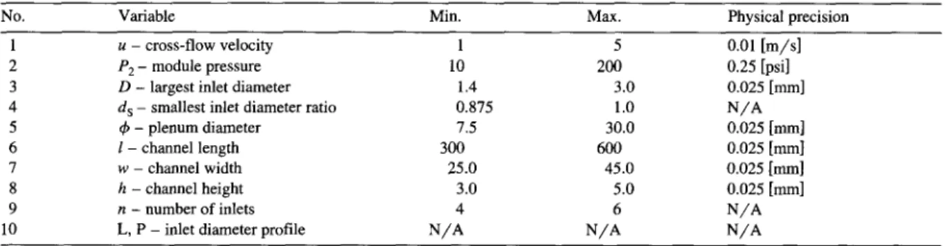
In view of the P1 constraint, the highest cross-flow velocity allowed was 5 m / s and the smallest inlet diameter allowed was 1.4 mm. The largest inlet diameter was selected so as to be no larger than the smallest channel height considered, so as not to confound the subsequent statistical modelling. The channel width was selected to ensure that edge ef- fects were not significant over the permeation area. Table 3 shows the list of variables and their ranges used in the factorial design.
3.4. Experimental design
A full two-level factorial design with 10 parame- ters requiring 21° (1024) simulations was used for an initial screening. This is an effective way to mini- mize the number o f simulations required to check on all possible variable interdependencies. Fractional two-level designs were not considered as the as- sumption of insignificant high order interactions was suspect. Three-level or central composite designs were excluded at this stage as the profile type had two levels and the number of inlets was a discrete variable.
An initial examination of the responses from the 10 variable screening study yielded some steps to- wards an ultimate design. Using coded variables, the operational parameters were always found to give a worst case result at (u, P 2 ) = ( + 1, - 1 ) for both
Table 3
Factoral design variable ranges and associated physical precision
No. Variable Min. Max. Physical precision
1 u - cross-flow velocity 1 5 0.01 [m/s]
2 *°2 - module pressure 10 200 0.25 [psi]
3 D - largest inlet diameter 1.4 3.0 0.025 [ram]
4 d s - smallest inlet diameter ratio 0.875 1.0 N/A
5 4) - plenum diameter 7.5 30.0 0.025 [turn]
6 l - channel length 300 600 0.025 [ram]
7 w - channel width 25.0 45.0 0.025 [mm]
8 h - channel height 3.0 5.0 0.025 [ram]
9 n - number of inlets 4 6 N/A
K. Darcovich et al. / Journal of Membrane Science 124 (1997) 181-193
189
design criteria. Further, best results were uniformly obtained at l = + 1. By inspection, stable local min- ima of the data occurred when n = - 1, that is, with four channel inlets. The linear and parabolic inlet diameter profiles yielded near identical results, so that the linear profile was chosen for simplicity. Thus, the number of design variables was reduced to only five, as it was only necessary to evaluate each design for the operating conditions (u, P 2 ) = ( + 1,
- 1 ) .
At this stage, further consideration was given to the pumping requirements for the envisioned module design. Based on the initial screening study, the velocity response was qualitatively expected to be minimized with a large channel width. Coupled with a large channel height, this resulted in an excessively large pumping requirement at the highest cross-flow velocity. The channel height was fixed at the center point, which yielded an acceptable pressure drop response of 3.9%. This reduced the module design variables to four.
The two responses were modeled with a multi- variate regression routine (IMSL: DRGLM). The general linear functional form for a response y; (either velocity standard deviation YVEL or pressure drop YPRESS) would be: (below, j, k, L m = 1, 2, 3, 4) Yi = tO q- fljX 1 d- fljkXjXk -I- [~jklXjXkXl
"~ ~jklmXjXkXlXm @ ~
(1)
Since the data was generated by numerical simu- lation instead of physical experimentation, the vari- ance was zero. The absence of a stochastic term, e, in Eq. (1), or a reasonable external estimate of the response variances, necessitated simulating this vari- ance. A random number with a normal distribution N(0, 1) was multiplied by a variance estimate based on the physical precision expected during fabrication of the module, as given in Table 3. The three different sample variances of the two responses were estimated from 50 simulations with the design vari- ables varying randomly within their error ranges. Estimates were obtained with all the design parame- ters set at either their low, mid or high levels. The sample variances of the responses at a given level were calculated by:
N (Yij__y"~i) 2
s i = E
j=lv-1
(2)
The variance estimates obtained at the three levels were compared to see if they came from the same population. The ratio of the sample variances s 12/s
22
has an F probability distribution function with a 100(1 - ~)% confidence interval:
)
s~2fvl,vZ,~/2 ,
~22 F~l,V2,1_ ~/2
(3)
The value of the F statistic is 1.62 for these cases where v I and v 2 = 49 degrees of freedom associated with each sample variance. The significance of the parameter estimates in Eq. (1) can be determined by whether a 95% confidence interval contains 0:fli --- t0.05,,( Var
fli) 1/2
(4)where
t0.05,49
is the statistic taken from the t distri- bution with n degrees of freedom associated with Var/3 i, the variance of the i-th parameter and is estimated from the sample variance, Eq. (2) and the diagonal elements of the variance-covariance matrix for Eq. (1).Determining the significance of terms with the pressure drop response model was straightforward, only 4 terms were significant regardless of which variance estimate was used. These terms were all associated with the channel height. The remaining parameter estimates were essentially zero. The corre- lation coefficient (r-factor) for this model was > 0.99. This was expected as the pressure drop across the permeation area should not have been a strong function of the plenum design itself.
The significance of terms in the velocity response model was evaluated using the largest variance esti- mate which came from the case with all the coded variables at the - 1 level. The correlation coeffi- cient, r, for the velocity response model was 0.98, but with only 5 degrees of freedom. An adequate model could not be obtained without consideration of all the higher order interactions. Eliminating all parameter estimates for third and higher order inter- actions resulted in a very poor fit, r < 0.6.
The existing two-level factorial design was ex- panded to a full three-level design with the remain- ing four variables. Similar results were obtained with respect to the model adequacy and significance of parameter estimates. The typical quadratic model with second order interactions and quadratic terms
190 K. D a r c o v i c h e t a l . / J o u r n a l o f M e m b r a n e S c i e n c e 1 2 4 ( 1 9 9 7 ) 1 8 1 - 1 9 3
could not adequately describe the results, r = 0.68. If all the significant terms were included based on t-tests, the correlation coefficient was high ( r = 0.98) but only because all but 3 out of 81 possible terms were retained. This suggests that the interactions between the remaining variables are complex.
At this point, the module design was further refined by inspecting the simulation results. The module width was set to the upper level (45 mm) as the velocity response was always lower at this level. This level was always obtained using a bounded function minimization routine (IMSL: DBCOAH) with the quadratic model. The maximum inlet diame- ter was also fixed at the upper level (3 mm) to minimize the pressure in the plenum. Smaller inlet diameters required a plenum pressure > 1000 psi for cases with the maximum cross-flow velocity. This restriction did not penalize the velocity response.
The plenum diameter, ~b, and the smallest inlet diameter ratio, d s, were the two remaining design
variables. The response surface for these variables could only be adequately described by a full quadratic model, again suggesting strong interactions between these two design variables.
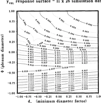
The predicted response (YvEL' Fig. 7) surface was verified by running the flow simulation for an 11 × 26 grid covering the region of the two final coded variables, Fig. 8. The velocity response is a weak function of d s over a large part of the region stud- ied. A maximum in YVEL occurs across the range of ~b. For large plenum diameters (~b = + 1), the inter- nal pressure equilibration is very even, providing near constant module inlet velocities contributing to flow uniformity. As ~b decreases, the pressure equili- bration worsens, as higher feed pressures, P1, are required. This causes an increase in Yv~L. However, as 4, further decreases, from - 0 . 5 to - 1 , P1 in- creases to the point where the pressure acting at both ends of the plenum is sufficiently high relative to the overall plenum pressure drop (P1 - P 2 ) .
A Y V E L r e s p o n s e s u r f a c e - 3 l e v e l f a c t o r i a l m o d e l 0 t~ ° ~ v 1.00 0.75 - 0 . 5 0 -
- - . - Q ... o.--'---o oo. ... o.oo~ ~ o . o o 2 On "uo$ . . . . " ~ 0 ^- u.O03 . . . . 0 003 . . . .... "v06 ... 0 O0 "uu4"~--~-O 004 - " 0 ~ ' 0 - S ... 0 • - 0 . 0 0 4 ~ "007 .006_..._._ .005 .... 0 005 . . . 0 005 . . . . ... ~'0.008 " " .0.007 ~ 0 . 0 0 6 . ~ _ _ ~ 0 . 0 0 6 ~ _ 0 . 0 0 6 ~ _ . ~ ... 0.007 . 0"00. 0.008 0 . 0 0 7 . . . 0 . 0 0 7 . . . ~ o ~ " " Oo ~ 0 " 0 0 8 " ~ - ~ - - 0 0 0 0 - 0 . 0 0 8 ~ .01 " 09 .. 0 .0.009 " O. 009 0.25 - " ~ o ... 0.009 ... 0 009 ....
!
0 . 0 0 - ) - 0 . 2 5 - j ~ ' . o O ° 9 ... 0,009 . • 0 . 0 0 9 • b~'O O.°Oq " " " " .... - 0 . 5 0 - 0009 ~ o . O o 0 ~ o.oo8 o. oo8 ---____ 3 0 8 / 0 . 0 0 8 | ~ 0 . ( ... 0 . 0 0 7 . . . . 0 . 0 0 7 . . . 0 . 0 0 7 . . . .... o.O0'r .... - - 0 . 7 5 - o . 0 O T .... 6___.__._0 0 0 6 ~ 0 0 0 6 ~ 0 " 0 0 6 - - | " 0 0 0 6 - - - ~ 0 " 0 0 . . . 0.005 . . . 0 . 0 0 5 0"005 . . . 0 . 0 0 5 . . . O.UU;~ / 0 . 0 0 4 ~ 0 . 0 0 4 ~ -t.O0 , , ~ ' ... i ... - 1 . 0 0 -0'.75 - 0 . 5 0 - 0 . 2 5 0100 0'.25 0.50' 0.75 1.00 d ( m i n i m u m d i a m e t e r f a c t o r ) SK. Darcovich et al. / Journal o f M e m b r a n e Science 124 (1997) 1 8 1 - 1 9 3 191 YVEL r e s p o n s e s u r f a c e - 11 x 2 6 s i m u l a t i o n d a t a 1 . O 0 ~ 0.75
I ~
~
\ ° . o ~ . ° O o s - ' ~0.50t
... . I ~ . ,oo~-~°~°s~:~--o.o_o~__ - - ~ " " l - - - ~ " ~ - o nn, ... ~ l . . . o o i s . • O . f l l S . . . /1 N I ~ . . . t l N I ~ . . . N ¢ t l ~ . . . " - - - ~ - - - 0 " 0 1 6 ~ 0 0 1 6 O O l ~ O f l l ~ , f l f i l 6 - - 0 . 2 5 - " . . . 0 . 0 1 7 . . . 0 . 0 1 7 . . . 0 . 0 1 7 . . . 0 . 0 1 7 . . . 0 . 0 1 7 . . . - - ~ - - - - ~ 0 . 0 1 0 0 . 0 1 8 ~ . j . 0 . - ~ 1 8 0 " 0 ~ 1 8 - 0 . 0 1 8 = = = - - ~ 0 . 0 1 8 ~ 0 . 0 1 8 - - - ~ ' - - 0 . 5 0 - a n . n 1vn . . . . a l " ~ ~ 1. . . . 7 0 . 0 1 7 ~ 0 . 0 1 0 " 0 1 7 6 - ' - - - . . . . . . o.,o,,~ .... o . " " , o ~ o - ° " ~ ' " ' " -- ~o.~ . . . ... ~ v . v , v ~ . . . . . . v u t ~ ' l / u . ~ t n - 0 . 7 5 - ~ =:=~7 ~ : = : ~ : : : z : . . . . ::::~ ~ = = 7 , 7 ... . . . . " v u o ~ U . . n o u ' ( u v u o u u.JO . . . • v . u u u o ~ U . u . . . . u . u o u . I j U 4 - - U I U U O / U I ~ U ~ . . . UIUUa" UIUU4 / . . . -1.00 ~'tL'7, ~ u , ~ ; , - 1 . 0 0 - 0 . 7 5 -0.50 -0.25 0.00 0.25 0.50 0.75 1.00 d s ( m i n i m u m d i a m e t e r f a c t o r )Fig. 8. YV~L response surface for the coded range of 4) and d s generated from the numerical flow simulation run over an 11 × 26 grid of points.
The true and predicted response surfaces are simi- lar for values of ~b > 0. There is poor agreement when - 1 < ~b < 0. The maximal ridge near 4) ~ 0.4 was not predicted by the model since the 23 design did not provide any data in this region. This suggests that a third or higher order model is required to adequately represent the true response surface. It has not been uncommon for other multi-variable experi- mental design models to be highly complex [11,12]. Hsu [13] conducted a 9-variable study of surimi processing using a central composite design. The significant lack of fit can be attributed to the omis-
sion of cubic a n d / o r higher order interaction terms. In view of these previous findings, it was more reliable to use the YVEL contours (Fig. 8) for any further design considerations.
3.5. Final parameter selection
Depending on the starting point, the function min- imization routine (IMSL: D B C O A H ) arrived at the points ( d s, ~b) = ( + 1, - 1) or ( + 0 . 9 6 , + 1). Exami- nation of the true response surface (Fig. 8) at these points led to the selection of ( d s, ~b) = ( + 0.96, + 1)
Table 4
Finalized values for each design parameter
Width of Height of Diameter of Smallest inlet Largest inlet Length of Number of Linear/ channel (ram) channel (ram) plenum (ram) diameter ratio diameter (ram) channel (cm) inlets parabolic
192 K. Darcovich et al. / Journal of Membrane Science 124 (1997) 181-193
for the final module design parameters. The velocity distribution predicted for the ~b = - 1 case for the outlets, (i.e., the u i values) was a sharp decreasing profile in this case. For the larger plenum case, a very uniform Ug distribution was obtained, owing to the better internal pressure equilibration. Further, the YVEL response surface has contours more widely spaced at the ( + 0.96, + 1) minima than at the ( + 1, - 1) minima, indicating better stability and less sen- sitivity to system or physical perturbations. The dif- ference between d s = + 0 . 9 6 and d s = + 1 . 0 in physical terms amounts to inlet diameter increments of 0.03 m m per hole. This length is roughly the machining precision, so for practical considerations, the final value of d s = + 1.0 was chosen.
The final design values for each parameter are given in Table 4. Note that the simulations were done using a half-width model assuming symmetry, and the values given below are for the entire module. Corresponding to the parameters in Table 4, the worst case responses were: YvE~ = 0.00100, Y~Ess = 0.0374, obtained under the operating conditions of P2 = 10 psi and u = 5 m / s . The largest value of P~ (347.7 psi) occurred at P2 = 200 psi and u = 5 m / s . 3.6. Response stability
With the chosen design parameters, the stability of the responses at the extremes of the operating variables was investigated. The CFD simulation was run 25 times at these points with fluctuations corre- sponding to the expected physical precision, as were given in Table 3.
At the outset, general notional criteria were to keep the response variables below 5%. In view of this, even in the worst case, both responses YVEL and YPRESS fall within this bound, as shown in Table 5.
Using the finalized physical dimensions, work will begin to construct this module.
4. C o n c l u s i o n s
A thin channel cross-flow module with a uniform flow field was designed for the characterization of flat ceramic membranes. A total of ten variables were considered for the module design. A 21° facto- rial design was used to evaluate the predicted mod- ule performance for each combination of the design variables.
It was found that running the simulation at the highest cross-flow velocity and the lowest module pressure always resulted in the worst-case perfor- mance for a given module design. Based on the screening study, it was possible to fix l = + 1, and n = - 1 with a linear inlet diameter profile. At this point, consideration of pumping requirements led to setting h = 0.
Inspection of the subsequent results from a more focused three-level factorial design in the remaining four module parameter variables was able to fix w = + l, and D = + 1. A response surface analysis in the final two module parameters determined opti- m u m values of d s = + 1 and t h = + 1.
Throughout the design process, a suitable regres- sion model for YvEL was not obtained because of the highly irregular response surface. However, the ex- perimental design approach did provide the data necessary for decisions to fix the design parameters. A sensitivity analysis of the proposed design showed that it is stable for the full intended range of operating conditions. Thus, its desired performance can be achieved with some margin of safety.
5. L i s t o f s y m b o l s
Table 5
Response error ranges for the extreme points of the operating variables u P2 YVEL Y ... P~ (psi) --1 --1 0.00097+0.00007 0.0015+0.0002 15.9+1.1 --1 + 1 0.00096+0.00007 0.0001 +0.0000 205.9+ 1.1 + 1 -- 1 0.00100+__0.00006 0.0374+_0.0015 158.0±5.0 +1 +1 0.00099+0.00006 0.0013±0.0000 347.7±5.0 A , B , C ds D D1,D2 F
coefficients of the parabola for grid genera- tion
smallest inlet diameter largest inlet diameter
diameters o f the adjacent inlets for grid gen- eration
statistic from probability distribution for ratio of two independent chi-square distributions
K. Darcovich et al. / Journal of Membrane Science 124 (1997) 181-193 193
f,
h i i,j,k l f L n ?l V N P P1 P2 P3 A Pa
F R e s i t u ui u i U u w YG, Yi Yij YPRESS YVEL WVELfanning friction factor channel height
subscript: relates to inlet number subscripts: tensor spatial indices channel length
distance between two inlets length along plenum number of inlets
number of velocity nodes which fall over the permeation region of the membrane
variance calculation sample size pressure, in transport equation
pressure to be delivered by pump for plenum inlet
pressure at front end of module channel pressure at exit of module channel pressure drop across module volumetric flow rate
correlation coefficient, measure of systematic association between two variables
Reynolds number sample variance
statistic from probability distribution function for a normal distribution with unknown vari- ance
cross-flow velocity module inlet velocity
average velocity at module front end velocity used in determining uniformity re- sponse
velocity in plenum channel width
x c orthonormal unit vectors for grid generation average Yi
j-th response in variance calculation for Yi simulation pressure response
simulation velocity response model estimate of velocity response
5.1. Greek letters OL
fl
~ijk .... ~ij srsc /x significance levelproportional coefficient for grid generation elevation coefficient for grid generation multivariate regression coefficients Kronecker delta function
screen drag coefficient fluid viscosity
u degrees of freedom p fluid density
Tij,j shear stress tensor
~b
plenum diameterReferences
[1] W.-M. Lu, K.-J. Hwang and S.-C. Ju, Studies on the mecha- nism of cross-flow filtration, Chem. Eng. Sci., 48 (1993) 863.
[2] C. Kleinstreuer and G. Belfort, Mathematical modelling of fluid flow and solute distribution in pressure-driven mem- brane modules, in G. Belfort (Ed.), Synthetic Membrane Processes. Fundamentals and Water Applications, Academic Press, New York, 1984, pp. 131-190.
[3] J. Robert, R. Giinter and J. Hapke, Optimization of flow design in a plate type membrane module system by means of a video camera, in R.A. Bakish (Ed.), Proc. 4th Int. Conf. Pervaporation Processes Chem. Ind., Mater. Corp., Engle- wood Cliffs, NJ, 1989, pp. 554-564.
[4] S. Harada, Hollow-fiber module container for reverse osmo- sis, Japan Patent, No. 60-261506 A2, 1985, 3 pp.
[5] S. Yoshikawa, K. Ogawa and S. Minegishi, Distributions of pressure and flow rate in a hollow-fiber membrane module for plasma separation, J. Chem. Eng. Jpn., 27 (1994) 385. [6] D.F. Boucher and G.E. Alves, Fluid and particle mechanics,
in R.H. Perry and C.H. Chilton (Eds.), Chemical Engineers' Handbook, 5th edn., McGraw-Hill, New York, 1973, pp. 5-1-5-65.
[7] K.Y.M. Lai, TURCOM: A computer code for the calculation of transient, multi-dimensional, turbulent, multi-component chemically reactive fluid flows. Part I: Turbulent, isothermal and incompressible flow, NRCC, Division of Mech. Eng., Technical Report NRC No. 27632, TR-GD-011, 1987. [8] E. Pellerin, E. Michelitsch, K. Darcovich, S. Lin and C.M.
Tam, Turbulent transport in membrane modules by CFD simulation in two dimensions, J. Membrane Sci., 100 (1995) 139.
[9] B. Carnahan, H.A. Luther and J.O. Wilkes, Applied Numeri- cal Methods, Wiley, New York, 1969.
[10] I.E. Idelchik, Fluid Dynamics of Industrial Equipment: Flow Distribution Design Methods, Hemisphere Publ. Corp., New York, 1991.
[11] M.J. Haas, D.J. Cichowicz, J. Philips and R. Moreau, The hydrolysis of phosphaticylcholine by an immobilized lipase: Optimization of hydrolysis in organic solvents, JAOCS, 70 (1993) i l l .
[12] T.S. Moss, W.J. Lackey and G.B. Freeman, The chemical vapour deposition of dispersed phase composites in the B - S i - C - H - C I - A r system, Mater. Res. Soc. Symp. Proc., 363 (1995) 239.
[13] S.Y. Hsu, Optimization of the surimi processing system with a central composite design method, J. Food Eng., 24 (1995)