Approaches to Optimal Inertial Instrument
Calibration using Slewing
by
Theresia C. Becker B.S. Mechanical Engineering
B.A. Medical Applications of Engineering Boston University, 2003
SUBMITTED TO THE DEPARTMENT OF AERONAUTICS AND ASTRONAUTICS IN PARTIAL FULFILLMENT OF THE REQUIREMENTS FOR THE DEGREE OF
MASTER OF SCIENCE IN AERONAUTICS AND ASTRONAUTICS AT THE
MASSACHUSETTS INSTITUTE OF TECHNOLOGY JUNE 2005
( Theresia C. Becker, 2005. All rights reserved.
The author hereby grants to MIT permission to reproduce and distribute publicly paper and electronic copies of this thesis document in whole or in part.
/
7
Signature of Author:.
/I,
Department of Aeronautics and Astronautics
May 6, 2005
Certified by:.
Matthew Bottkol Principal Member of the Technical Staff, C. S. Draper Laboratory
Thesis Supervisor ?
K
Certified by
George Schmidt Lecturer in Aeronautics and Astronautics
Thesis Supervisor I I, Accepted by MASSACHUSETTS INSTD E OF TECHNOLOGY DEC 012005 i i iiE
I
ls
e - x Jaime PeraireProessor of Aeronautics and Astronautics Chair, Committee on Graduate Students
ARCHIVES ./ .. ... _~~~~~~~~~~~~~~~~~~~~~~~~~~~~~~~~~~~~~ ft : i~~~~~~~~~~~~~~~~~~~~~~~~~~~~~~~~~ ' -I r I
Approaches to Optimal Inertial Instrument Calibration using
S lewing
by
Theresia C. Becker
Submitted to the Department of Aeronautics and Astronautics on May 6, 2005, in partial fulfillment of the
requirements for the degree of
Master of Science in Aeronautics and Astronautics
Abstract
Calibration of an inertial measurement unit is important to the success of accuracy-sensitive missions. This thesis analyzes calibration techniques for two inertial measure-ment mechanizations: (1) an inertially stabilized system and (2) an inertially referenced slew. An inertially referenced slew rotates the inertial measurement unit with respect to an inertial reference frame independent of the vehicle motion. The appropriate inertially referenced slew is determined by a proposed optimal calibration method that maximizes the correlation between a measurement and a covector, specifying a mission performance indlex. The performances of a six-position dwell calibration (inertially stabilized system) and an optimal slewing calibration (inertially referenced slew) are determined to be de-pendent on the mission. The inertially stabilized system is preferred for determining accelerometer errors and an inertially referenced slew is preferred for calibrating rate-sensitive gyroscope errors.
Thesis Supervisor: Matthew Bottkol
Title: Principal Member of the Technical Staff, C. S. Draper Laboratory
Thesis Supervisor: George Schmidt
Acknowledgments
I would first and foremost like to thank the Charles Stark Draper Laboratory for giving me a place to foster my knowledge and development as an engineer. It would be difficult to overstate my gratitude to my thesis advisor, Matthew Bottkol. With his inspiration, he has motivated and encouraged me to explore innovative solutions. Tom Thorvaldsen and Howie Musoff have been a great resource to provide an overview of prior-free calibration problems. My MIT advisor, George Schmidt has been very supportive throughout my time at Draper. I would also like to thank Richard Phillips and Michael Luniewicz for guiding me through projects in dynamics and controls and broadening my knowledge in aeronautics and astronautics.
I would also like to thank everyone at Boston University. They nurtured my growth as a person and as an engineer. I am especially grateful to Anil Rao for providing me with the foundations for dynamics and Pierre Dupont for his expertise in controls.
I thank my friends Judy Henry and Hendrik Herold. They have provided me with unconditional support throughout the term of this project. Also, thank you Draper Fellows for your advice and company, especially Gordon Thompson and Sara MacClellan. Finally, I would like to thank my parents and family for their inspiration and support
throughout my life.
This thesis was prepared at The Charles Stark Draper Laboratory, Inc., under Contract N00030-05-C-0008, sponsored by the U.S. Navy Strategic Systems Program.
Publication of this thesis does not constitute approval by Draper or the sponsoring agency of the findings or conclusions contained herein. It is published for the exchange and stimulation of ideas.
Contents
1 Introduction
1.1 Navigation and Calibration 1.2 Initial Calibration .
].3 Centrifuge Calibration . . . 1.4 Thesis Overview...
2 Kinematics and Estimation
2.1 Inertial Navigation ... 2.2 Navigation Equations . 2.3 Kalman Filter ... 2.4 Covector Estimation ....
3 Slewing Maneuver
3.1 Analysis of Slewing Maneuver ... 3.2 Baseball Stitch Slew ... 3.3 Example Problem . ...
4 Problem Formulation
4.1 Prior-Free Estimation Problem.
4.1.1 Prior-Free Estimation considering all IMU Errors ... 4.1.2 Prior-Free Estimation considering Mission-Specific Trajectory
11 11 13 13 14 17 17 18 19 22 25 25 27 28 31 32 34 34
...
...
...
...
...
...
...
...
4.2 Calibration with Prior Knowledge . . . .. .... . 35
4.2.1 Calibration with Prior Knowledge considering all IMU Errors . . . 36 4.2.2 Calibration with Prior Knowledge considering Mission-Specific
Tra-jectory ... 36
5 Theoretical Developments 37
5.1 Optimal Angular Velocity to Improve Measurements ... 37 5.2 Optimal Angular Velocity and Steepest Descent ... 39
6 Results
6.1 Performance of Individual Errors ... 6.2 Slewing Mission.
6.3 Inertially Stabilized Mission ...
7 Conclusion 7.1 Future Research ... A Quaternion Algebra
B Initial Errors
C Kronecker Products
41 41 47 49 51 52 55 57 59 8List of Figures
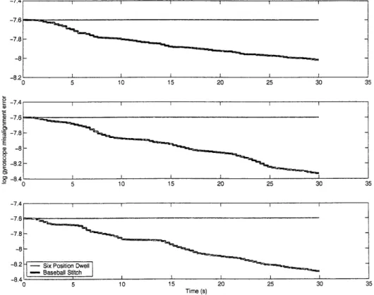
6-1 Gyroscope Misalignment Errors along 3 Axes after Calibration ... 42
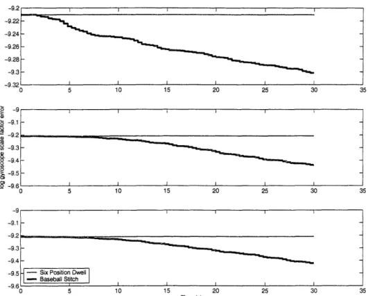
63-2 Gyroscope Scale Factor Errors along 3 Axes after Calibration . ... 43
6-3 Gyroscope Bias Errors along 3 Axes after Calibration . ... 43
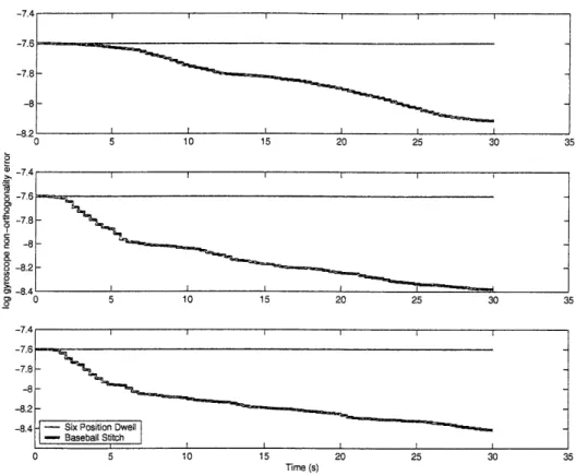
6-4 Gyroscope Non-Orthogonality Errors along 3 Axes after Calibration... 44
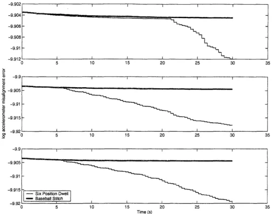
6-5 Accelerometer Misalignment Errors along 3 Axes after Calibration .... 45
6-6 Accelerometer Scale Factor Errors along 3 Axes after Calibration. ... 45
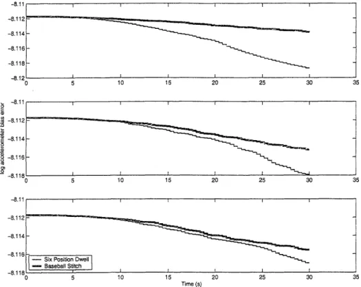
6-7 Accelerometer Bias Errors along 3 Axes after Calibration ... 46
6-8 Accelerometer Non-Orthogonality Errors along 3 Axes after Calibration. 46 6-9 Performance Index versus Time given a Slewing Mission. . ... 48
Chapter 1
Introduction
1.1 Navigation and Calibration
Inertial navigation is the process of determining the position, velocity, and attitude of a vehicle from inertial data. An inertial measurement unit (IMU) is a system of instru-ments that gathers the necessary navigation data. Specifically, the IMU instruinstru-ments are orthogonal triads of accelerometers and gyroscopes that respectively detect the specific force and angular rate of the vehicle. The instrument outputs are integrated to track the vehicle's position, velocity, and attitude. The accuracy of the IMU instruments limits the ability to navigate; therefore, the instruments are calibrated prior to flight.
Calibration is the determination of error characteristics. The relationship between the instrument outputs and the known, theoretical values is described by error characteristics or more specifically, instrument errors. Calibration makes the instrument errors observ-able, distinguishes them, and adjusts the instrument model according to these errors. "A control system is said to be observable if, for all initial times, the state vector can be de-termined from the output function, defined over a finite time." [8] Individual instrument error observability is essential in instrument calibration. Calibration of gyroscopes and accelerometers for aerospace missions such as missile guidance require tolerances on the
order of micro g's and microradians.
As a simple example consider accelerometer calibration. If the errors are limited to bias and scale factor, then these errors can be observed by the following procedure. First, the accelerometer is placed with its input axis in the vertical direction and the output is integrated over time. The combined effects of bias and scale factor are observable, but the errors cannot be distinguished. If the calibration is repeated with the input axis reversed, the bias and scale factor contributions can be separated. The error characterization of the accelerometer bias is an additive quantity independent of the acceleration direction; whereas, the scale factor contribution is proportional to the acceleration that changes sign when the accelerometer input axis is reversed. This example is a simple case where the mechanism can be understood exactly.
In the 1960's, Dr. Rudolph Kalman developed a linear estimator or Kalman Filter. The optimal filter uses initial conditions, system and measurement dynamics, and statis-tics of system noises and measurement errors to determine the minimum error estimates of the system [3]. Correlations between the measurements and the instrument errors produce observable states. The Kalman Filter is used to determine individual errors for complicated systems with possibly hundreds of instrument errors. The calibration of these instrument errors yields accurate navigation during the mission.
The two basic navigation methods are a strapdown and an inertially stable system. Angular velocity of a strapdown system is that of the vehicle with respect to an inertial reference frame. An IMU on an inertially stable platform has gimbals, which essentially null the angular velocity with respect to an inertial reference frame. This thesis will not evaluate a strapdown system; instead, this thesis will compare an inertially stable system with an inertially referenced slew. An inertially referenced slew is a system that rotates with respect to an inertial reference frame independent of the vehicle motion.
This thesis will evaluate the initial calibration and the mission navigation. The per-formance of the calibration method will be compared given a specific method for mission
navigation. The mission navigation with an inertially referenced slew is a current area of
interest in navigation [4, 5, 7].
1.2 Initial Calibration
One example of a mission application is a ballistic missile, which requires a high level of accuracy to hit the target. This level of accuracy requires the accelerometers and gyroscopes to be calibrated within micro g's and microradians. There are several standard calibration techniques implemented to calibrate the instruments.
One method uses a shaker table, which vibrates the IMU at a given frequency. The characteristics of the IMU are compared with the output characteristics of the shaker table. In order to excite different errors along various axes, the test must be repeated
several times at different orientations.
Another method for calibrating an IMU prior to flight rotates the instruments using a centrifuge. The IMU position is measured at six points along the centrifuge path to calibrate the instrument errors. Similar to the shaker table, this test is repeated multiple times to excite different errors along different instrument axes. This thesis will focus on
evaluating and improving calibration of an IMU prior to flight using a centrifuge.
1.3 Centrifuge Calibration
In a typical calibration of an inertially stabilized IMU, the unit is attached to the arm of the centrifuge and spun at a specified rate for a given amount of time. Position measurements of' the IMU are taken at six points along the path of the centrifuge to calibrate the instruments. The IMU is then reoriented and the test is repeated. This procedure requires typically six different orientations of the IMU to observe the instrument errors.
of the IMU. First, the centrifuge must be restarted between each test. Also, it may not be valid to use the calibration of the previous orientation as the initial conditions for the next test. In order to accurately calibrate the IMU, this thesis considers slewing the IMU as it is being spun by the centrifuge. This mode of calibration applies particularly to missions that navigate using an inertially stabilized slew.
One disadvantage of this technique is the required modeling of more gyroscope states during an inertially referenced slew, since the IMU is rotating through a trajectory. The gyroscopes are on an inertially stable platform; therefore, during a test without slewing these rate-dependent gyroscope errors are not observable. In the slewing system, the IMU behaves more like a strapdown system than an inertially stable system. In order to correctly determine the angular rates, it requires modeling the rate-dependent gyroscope errors.
1.4 Thesis Overview
This thesis will discuss approaches in determining an optimal calibration method given a mission dynamics profile. The advantages of slewing trajectories for calibration are exam-ined. Specifically, the baseball stitch slew has inherent advantages and will be evaluated. The results for using such a trajectory are promising, but could be improved by other possible slewing trajectories. A method for determining an appropriate slewing trajec-tory is discussed, which uses prior covariance information. The results of both mission navigation methods (inertially stable and inertially referenced slew) are discussed to gain insight into the appropriate calibration technique (inertially stable or inertially referenced
slew) for each.
Chapter 2 is the foundation for the simulation including the navigation equations, Kalman filter, and mission covector formulation. The following chapter examines a gen-eral slewing maneuver and looks more closely at the baseball stitch slew. In Chapter 4
a method for determining an optimal slewing trajectory is presented based on prior co-variance information. The theoretical formulation of this optimal slew and an evaluation of the method is discussed in Chapter 5. Chapter 6 presents the results of the thesis and the conclusion is discussed in Chapter 7.
Chapter 2
Kinematics and Estimation
Inertial navigation requires knowledge of the system's kinematics and possibly, additional external measurements. In centrifuge calibration the difference between the predicted and measured position creates observability of the instrument errors. An optimal estimator, or Kalman Filter, uses this observability to determine the minimum variance estimates and to calibrate the instruments. The calibration performance may be assessed using a covector or linearized performance index, such as miss distance.
2.1 Inertial Navigation
T'he two basic navigation methods are a strapdown system and an inertially stable system. A. st:rapdown system is rigidly attached to the body of the vehicle; therefore, the vehicle's angular velocity is the nominal angular velocity of the gyroscopes. An inertially stabilized system has a nominal angular velocity of zero, because the gimbals essentially null the rotational effects. This thesis will consider an inertially referenced slew, a method where the IMU is isolated from the vehicle attitude with a stabilized platform. The gimbals drive the platform through a predefined inertial attitude history with nonzero angular rates. In the inertially referenced slew the gyroscopes nominally output the angular velocity of the slewing maneuver. This thesis will consider an inertially stabilized system and inertially
referenced slew.
2.2 Navigation Equations
The centrifuge navigation equations of the position x, velocity v, and attitude q in an earth centered, earth fixed frame (ECEF) are described by the following differential equa-tions
:E = VE (2.1)
VE
= fPqP- - 22E x vE - QE X (E X XE) (2.2)qE 12 0 qE (2.3)
where u is the gravitational constant, QE is the angular velocity of the Earth, and Equation 2.3 is a quaternion equation (Appendix A).
The superscript denotes the reference frame, where E is a reference frame that rotates with the Earth and P is a reference frame rotating with the platform of the IMU. The accelerometers measure specific force, f in platform coordinates; therefore, this must be rotated into Earth coordinates (Appendix A). The gyroscope measures angular velocity with respect to an inertial reference frame. To find the rotation from Earth to platform coordinates, Earth rate must be subtracted from the gyroscope output (QG).
When the IMU is mounted on the arm of a centrifuge, the earth relative position and velocity of the IMU at any point in time, t are modeled as
x = ro + ra(cos(wt)uN + sin(wt)uE) (2.4)
v = raWc(-sin(wt)uN + cos(w~t)uE)
(2.5)
where UN and UE are the unit vectors point North and East, respectively. r is the
vector from the center of the Earth to the center of the centrifuge. In this simulation, the centrifuge arm (ra) is assumed to be 10 m long and rotates at 2.6 rad/s, wc.
The attitude is dependent on whether the IMU is undergoing a slew or not. If there is no slewing maneuver, then the attitude is inertially constant since the IMU is on an inertially stabilized platform. If there is an inertially referenced slew, then the attitude of the IMU is determined by that specific maneuver relative to inertial space.
2.3 Kalman Filter
A Kalman filter uses initial conditions, system and measurement dynamics, and statistics of system noises and measurement errors to determine the minimum error estimates on the system [3]. In the following simulation, the performance of the inertial measurement unit will be described by 33 error states x. Error states 1-9 describe the dynamics of the system, error states 10-21 describe the gyroscope instrument errors, and error states 22-33 describe the accelerometer instrument errors as shown below. The gyroscope and accelerometer instrument errors are assumed to be constants.
x = (1-3) position
(4-6') velocity
(7-9 ) attitude
(10-12) gyroscope misalignment (13-15) gyroscope scale factor (16-1:L8) gyroscope bias
(19-21) gyroscope non-orthogonality (22-24) accelerometer misalignment (25-27) accelerometer scale factor (28-30) accelerometer bias
The Kalman Filter measurement update to the state and covariance, respectively are
Xk
= x +
Kk(Zk
- Hkx )
(2.6)P+ =
(I-
KkHk)P (2.7)where the measurements are
Zk = Hkxz + Vk (2.8)
and the Kalman Gain is
Kk = P Hk (Hk P7 Hk + Rk)- (2.9)
Vk is the measurement error, where E[VkvT = Rk. Hk is a matrix corresponding to the states that are being measured. In the centrifuge case, the position is measured; therefore,
Hk=
/(3x3) o(3x3o) ] (2.10)The extrapolation of the states and covariance are described by
4+
Xk = TzXk (2.11)(2.12)
where Q is the process noise, which in this simulation is velocity random walk.
For small time steps where F(t) is approximately constant, the Taylor expansion of the exponential ) can be approximated by:
4?= eFt
I + Ft + F2at2
2 (2.13)
where F is the linearized differential equations satisfying
J = F6x (2.14)
where
0
I
0
0
0
0
0
0 00
-G--[QE] 2 -2[QEx]
-[fEx]R
0
0 0 0
[ffEx] f I E0 0 0 -[QPX] fQGIQG 0 0o 0 0
0 0 0 0 0 0 0 0 00
0 0 0 0 000 0 000
(2.15)
Process noise is not a part of the linearized differential equation, because it is not a significant factor in calibration. Process noise may increase or decrease the calibration time necessary, but it will not change the qualitative results of calibration performance.
rThe gyroscope and accelerometer errors are assumed to be random constants indepen-dent of time. Special notation has been used to denote a diagonal matrix and a symmetric matrix with zeros along the diagonal as seen below
wI wi 0 0 w= w2 = 0 w2 0 (2.16) W3 0 0 W3 and W/1 W /0 W2 W= W2 w3 0 W1 (2.17) W3 W2 W 0
A notation used throughout this thesis is [ x], which denotes
W1 0 -W3 w2
[WX= = W2 X = 3 0 -W1(2.18)
W3 --W2 i1 0
2.4 Covector Estimation
Instead of estimating the entire state, consider estimating a linear combination of states or ATx. A is a covector or a linear functional on a vector space. One common performance index is the circular error probability (CEP) of a ballistic missile, the radius of a circle into which the projectile will land at least half of the time. Instead of discussing CEP, this thesis will look at two other costates, the downrange and crossrange miss. Downrange and crossrange miss is the probability the missile will land within the miss distance away from the desired target 50 percent of the time.
The trajectory of a ballistic missile is determined by the differential equations for position x, velocity v, and attitude q in an ECEF coordinate system.
5CE = VE (2.19)
E E VE
= XE 3 + T E -2[QE X]vE- [QEX]2XE (2.20) 1P
2 *
= (QG-Q - -(2.21)*1)
qEwhere T is the thrust of the vehicle, which is assumed to be 8' g until it reaches an altitude of 30,000 meters. Once the vehicle has reached 30,000 meters, no external forces are acting on the vehicle except gravity. The range of this projectile is approximately 650,000 meters. In the inertially stable mission, the angular velocity of the gyroscope (QG) is 0. In the inertially referenced slew, the angular velocity of the gyroscope is defined by the slew
maneuver with respect to an inertial reference frame.
The unit vectors at impact UDR (downrange), UCR (crossrange), and uup (up) define a right-handed coordinate system. The earth-relative miss distances at t = tf are defined
by /XDR = UDRJX(tf) AXCR = UCRJX(tf) AXU = UTpJX(tf) (2.22) (2.23) (2.24)
The inertial misses at geometric impact, when the missile hits the earth's surface at Ixf I = RE are Ax impact / XD A~DR AXDR (2.25) A impact = XCR A~XC1 =-xc (2.26) nimpact O UP (2.27)
The covectors A1 and A2 in an ECEF coordinate system are defined as
(2.28) A1= UDR
j
0 0 (2.29) (2.30)Covectors can be propagated backwards in time by the linear transition matrix b based on the true angular velocity and specific force.
4D(tf, t) is the state extrapolation matrix used in the Kalman filter from the final time of
the projectile hits its target to the time of launch.
Chapter 3
Slewing Maneuver
Navigation mechanized with an inertially referenced slew is sensitive to gyroscope errors that are normally neglected in an inertially stable mechanization. An inertially stabilized calibration, such as a six-position dwell does not excite the rate-dependent gyroscope errors. A mission with an inertially referenced slew requires these gyroscope errors to be calibrated; therefore, a new method for calibration using slewing is required.
The first consideration for improving the six position dwell calibration is to compare it with a representative slewing maneuver. The so-called "baseball stitch slew" has the advantage of averaging the accelerometer bias; therefore, separating that error from the calibration problem. Desensitizing an error during calibration eliminates observability of this state over long periods of time and also eliminates cross-correlation between this error and other states. The advantage of eliminating cross-correlation is to improve observabil-ity of the other states, which as a result will improve calibration.
3;.1 Analysis of Slewing Maneuver
The accelerometer errors are analyzed to improve calibration by desensitizing accelerome-ter bias. The force error equation in ECEF coordinates, neglecting gravity can be written
as
6F = R0(t) (ba + saRO(t)F + [(Va + q) x]RT(t)F + (;aR(t)F) (3.1)
where q = RoT is the navigation attitude error expressed in body coordinates which is nominally constant if the rotation does not vary over short periods of time. R is the rotation matrix from the platform coordinate system to the ECEF coordinate system. The accelerometer errors ba, Sa, 4, and
Wa are the bias, scale factor, misalignment, and non-orthogonality, respectively.
The velocity error can be found by integrating the force equation
v(t) = F(T)d = ( Ro(r)d7 bA
+ i(Ro(T)aRo T(T))F(T)dT (3.2)
+
(RO(T)([(?a + ¢)x] +S)RT(r))F(T)dT
The accelerometer bias contribution disappears if
Ro (T) T= 0 (3.3)
To gain insight into the problem, assume that the force is constant and Equation 3.3 holds for trajectory Ro(t). In this case, the velocity error can be rewritten as
Av(T)= T MF
(3.4)
where M = 1 oT Ro()DR(T)dT with D = SA + [~aX] + [X ] + (a. The velocity error covariance contribution at the end of one period is
AP = E[Av(T)AVT(T)] = T2 F .2 E[MuFuTFMT (3.5)
Given a covector, A, the goal is to minimize
E
[(AT V(T))2] =AT AP
(3.6)
This is equivalent to minimizing the cost function J(Ro) where
J(Ro) = E [(ATMF)2] (3.7)
such that 0 = fo: Ro(r)dT
If Ro C X = {RI foT R(T)dr = 0}, then the problem can be reduced to finding a vector
vv(t) where
w(t) = Ro(t)DR
(t)uF(3.8)
is perpendicular to A for the maximum amount of time.
The above problem seems well-posed, but it has a constraint which makes the sample space very difficult to evaluate. Eliminating the constraint 0 = oT Ro(r)dT would allow one to search over the entire space of rotation matrices.
3.2 Baseball Stitch Slew
A baseball stitch slew has the property that 0 = f0TRo(r)dT, which will null the bias term
of Equation 3.2. The desensitization of the bias term will improve observability of other accelerometer errors by eliminating cross-correlations. A baseball stitch slewing maneuver is an inertially referenced slew that is a multiplication of two rotation matrices. The first rotation is about the z-axis with a frequency of w and the second is about the x-axis with
cos(wt) sin(wt) 0 - sin(wt) cos (wt) 0 0 0 1 1 0 O cos(2wt) O sin(2wt) 0 - sin(2wt) cos(2wt)
Using the rotation matrix relationship that JR = R[Q x], the angular velocity is
2w QBB = w sin(2wt)
w cos(2wt)
A baseball stitch slew is periodic, RBB(t + T) = RBB(t), and satisfies
T RBB(T)dTr = 0
o
(3.9)
(3.10)
(3.11)
The baseball stitch is a feasible not be the optimum. In the next discussed.
solution to the optimization problem posed, but may section, improvements on a given trajectory will be
3.3 Example Problem
The baseball stitch slew meets the required constraint that 0 = fT Ro(T)dT; however,
this slew trajectory may not be optimal for observing the remaining terms in Equation 3.2. Changing the total orientation of a feasible slew trajectory can improve observability. This example problem will examine a given feasible trajectory (R(r)) and find the total orientation (R) required to increase observability.
The total slew maneuver Ro(T) can be defined as Ro(-)- R(Rr). The total orientation
of the trajectory, R is independent of time. The trajectory itself is defined by R(T)
that satisfies = /T R(-r)dr; therefore, the total slew maneuver satisfies the feasibility
28 RBB(t) =
JT oT
I
TRo(T)dr
=o T
__R(T)dT = Rf
T
R(T)dr = 0
'The velocity error covariance contribution at the end of one period can be rewritten
AP
= T
2IF1
2.E
[(R(JT
R(T) DRT(r) d)1k
u)
(1 ( T Rt(T)DRT(T7
Using Kronecker products from Appendix C, the above can be rewritten as
[
((uFR
(A
R)
(ITR(r)DR
T()dT)
R( )DRT(r)dT)
= T2
IF
2(uR 0R)
. [( R()DRT)d) (jT )DRT(~)d) ~T](3.14)
where the underline denotes the matrix being written in vector form.
Note that AP is a 3 x 3 matrix, which is the velocity error covariance contribution at the end of one period T, due to initial scale factor, misalignment, and non-orthogonality errors. Suppose A is a given vector with norm one that corresponds to the minimum velocity error covariance contribution. Then, the problem can be formulated as a minimization problem, min ATAPA over a total orientation
A.
Substituting in Equation 3.14 for AP creates an optimization problem shown below.mi:n T2 F2.T(uj;l ®R).E
A ,RO). [ R(T)DR T (T
)d-)
jR(
T)DRT(T)dTr)
T(jT
" _ (U T(3.) TA (3.15) condition (3.12)A/P
= T
2F12 .E
-)d
(,3T
)
(3.13) T1 -jI)i(····-··T
'' -, \ I J /\-The above problem is equivalent to
min TWX (3.16)
where xT = AT(uTRo Ro) and W = E [(f R(T)DRT(T)d -) (frT R(T)DRT(T)d)]. Note that W is a known matrix based on initial errors and the given trajectory, and
|X| XT = AT(UTFR )(RTUF RT )A
= AT(U4RRTUF X TT)A
= AT(I
I)A
= A12
It was assumed that A = 1; therefore, Ix = 1. The solution to this minimization problem is the eigenvector, x that corresponds to the smallest eigenvalue of the matrix
W. To solve for , one must solve the equation x = (RTuF 0 RT)A, which can be
simplified
to
(
0
) = (UF
0
I)AXT.
Analyzing trajectories and improving observability provides insight into possible new trajectories that could create more observability. It is difficult to extend the simplified problem to determine other improvements on the slewing trajectories that are dependent on time, i.e. the optimal angular velocity. The optimization problem would require min-imizing over an integral of rotation functions, which cannot easily be accomplished using linear or nonlinear optimization techniques. Further analysis of the rotational subspace of slewing trajectories that have the property 0 =
foT
Ro(r)d - is required to determine if desensitizing the accelerometer bias is effective in calibration.Chapter 4
Problem Formulation
Chapter 3 discussed desensitizing errors to decrease cross-correlations between errors. Desensitization is only dependent on the kinematics of the vehicle. This chapter will focus on utilizing the optimal filter estimates to improve the calibration mechanization. The relationship between the measurements and the kinematics of the vehicle directly influence the observability of the error states and calibration.
Calibration can be divided into two separate categories. The first category uses only measurement information to determine the optimal future state. T. Thorvaldsen and H:. Musoff have addressed this prior-free case at Charles Stark Draper Laboratory using least-squares estimation. In this formulation, the least squares solution turns out to be identical to the prior-free Kalman Filter solution assuming no process noise. This approach lends itself to the six-position dwell calibration (inertially stabilized system), since the covariance from the previous test may not be appropriate in determining the next orientation.
The other category uses current state estimates to predict the optimal future state of the system that will obtain maximum observability. The relationship between the mea-surements and the kinematics of the system directly influence the observability in the future states; therefore, this relationship is used to formulate an appropriate
optimiza-tion problem. The unique work of this thesis uses current probabilistic informaoptimiza-tion to determine possible directions for improvement.
The categories can be further subdivided into two problems. The first problem min-imizes the errors over the entire IMU. Optimizing the entire IMU can be difficult and time consuming. From the error propagation and measurement update equations, it is very difficult to formulate a strategy to calibrate an IMU in this manner. However, this method assures that all errors are calibrated to the best ability.
The second problem minimizes the errors based on the final mission trajectory. The advantage of a mission-specific calibration is the ability to focus on calibrating the most significant errors, while neglecting those that have less weighting in the final objective, downrange and crossrange miss. The rate-dependent gyroscope errors are not significant during an inertially stabilized mission, but they are important in an inertially referenced slew mission. The most notable disadvantage of using this method, is the necessity for the trajectory to be fixed. In a ballistic missile trajectory calibrating specific states will not affect a slight change in mission planning.
4.1 Prior-Free Estimation Problem
To explore the prior-free estimation problem, consider the least squares problem. Let x E Rn be a Gaussian random variable with unknown statistics, norm x and covariance
P. Suppose we are given measurements z E Rm, then by the Kalman measurement update
z = Hx + v
(4.1)
where H is the measurement matrix and is Gaussian noise with known statistics
E[v'T] = R. Assume the measurements form an over-determined system and x is
observ-able. If x is observable, then the Grammian matrix G = HTH is invertible.
The weighted least-squared problem can be written as 1
J(x)
=-(z
-
Hx)TR-l(z
-Hx)
2 (4.2) The solution to J(x) isx= (HTR-1H)-lHTR-lz
(4.3)Note that the above equation is a function of the measurement and the measurement noise, not the current covariance or current measurement. This is the same as the Kalman estimate where the initial covariance matrix is infinite, or no prior knowledge of the states. The Kalman gain K can be written as
K = (p-l + HTR-lH)HTR-l
(4.4)Since the initial covariance matrix is infinite, then p -l 0 and
K
-K = (HTR-1H)HTR-1
(4.5)The Kalman measurement update is independent of the prior estimate of the state xo, such that the update is
= (I- KH)xo + Kz -- Koz
(4.6)Therefore, for the Kalman Filter prior-free limit the optimal estimate of x is
x = (HTR-1H)-iHTR-lz
(4.7)Ncote that Equations 4.3 and 4.7 are identical and the least squares update is identical to the prior-free limit of the Kalman Filter update assuming no noise. The estimated
covariance of the prior-free estimate is
P = (HTR
- 1H)
-1 (4.8)4.1.1 Prior-Free Estimation considering all IMU Errors
Assume the measurement noise covariance is a scalar measurement, R = a2I, then the prior-free estimate and covariance are given by a pseudo-inverse or
= (HTH)-lHTz
(4.9)P = iV(HTH)- ' (4.10)
Let the measurement matrix, H depend on a control variable u, then the optimization problem can be formulated as minimizing the trace of the covariance or
mintr ((HT(u)H(u))- 1)
4.1.2 Prior-Free
Estimation
considering
Mission-Specific
jectory
The objective function in Equation 4.11 may not be appropriate in all applications; there-fore, it may be desirable to have a mission-specific trajectory. As an alternative, suppose it is of interest to estimate a certain linear function of the state or
L(x) = ATX (4.12)
The estimate and variance of this function are
L
= AT(HT(u)H(u))-lHTz
(4.13) 34(4.11)
Tra-E[(L - L)2] = T(HT(u)H(u))-1' (4.14)
A covector A can determine the crossrange and downrange miss and the new optimization problem is defined as
min XT(HT(u)H(u))-1A (4.15)
4.2 Calibration with Prior Knowledge
IFuture states of the system can be estimated using the Kalman Filter equations. Using this estimate, the observability and calibration can be improved by maximizing the correlation between the measurements and the kinematics. If the trajectory of the IMU is fixed, consider optimizing the error estimates by controlling the type of measurements. Without process noise, the problem is to choose scalar measurement covectors H1, H2, ..., HN so
the measurements
Zk = HTX + Vk (4.16)
optimize the final covariance
1 1
PN=(HPO
+
HTH +...+
HNHk)
-1(4.17)
However, in the centrifuge calibration the measurements are fixed; therefore, it is ad-vantageous to control the system kinematics by slewing the IMU. As discussed in Chapter 2, the state transitions are
Xk = kXk-1
(4.18)
The Kalman Filter measurement update is
Zk = HTXk + (4.19)
rewritten as
PN= (Po +
(4.20)2 =i
4.2.1 Calibration with Prior Knowledge considering all IMU
Er-rors
To optimize the covariance in GPS satellite selection, one maximizes the information index
J(hl, h
2,..., hN) = tr(PN
1)
(4.21)
For IMU calibration, a similar idea can be used to maximize the information index or
maxtr (Po
++
E
nq:iHTHDT)
\i=1
(4.22)
4.2.2 Calibration with
Prior Knowledge considering
Mission-Specific Trajectory
It is of interest to estimate a linear function of the state such as
L(x) = ATx (4.23)
where A is a performance index to measure mission performance. In terms of the covari-ance, the cost function is
J(PN) = AXPNX (4.24)
To calibrate the mission-specific trajectory, it is ideal to minimize the objective func-tion with respect to 4i, or rewritten
n -1
Z
oiHTHo ) A i=1i36
Chapter 5
Theoretical Developments
Thle previous chapter discussed optimization to achieve global observability. Specifically, the results of Section 4.2 could require a different matrix at every measurement, which implies a new kinematic configuration to obtain optimality. This global optimization prob-lem is not practical for the centrifuge calibration. This chapter will focus on formulating a continuous trajectory based on the results of the previous chapter. The trajectory will not be predetermined (as in Chapter 3); instead, the slewing trajectory will be specified by continuous angular rates by maximizing the correlations between the measurements, the kinematics of the vehicle, and the covector.
5.1 Optimal Angular Velocity to Improve
Measure-ments
The impact of a measurement on mission performance is important to understanding observability. A scalar measurement update without noise can be written as
The measurement update is supposed to determine the errors of interest defined by a covector, A. A perfect measurement update along this covector would be
z2 = A Tx (5.2)
Taking the product of zl and z2
Z1 Z2 = h xZTA (5.3)
The expectation of Equation 5.3 results in
E[zl Z2] = hTPnA (5.4)
where Rn = E[XnxT] at measurement n.
For positive definite Pn, the Schwartz inequality ([2], [6]) states
IhTPnA < hTPih ATPA (5.5)
The equality holds when h and A are linearly dependent. If h = KA where K is a scalar constant, then IhTPnAl has reached its maximum and
IE[zi z] = I= 2 hTP = hTPh ATPA (5.6)
The maximum correlation exists when the measurement is along the covector of interest, which will result in a perfect measurement of the desired quantities.
Due to the dynamics of the centrifuge, it is impossible to ensure that h and A are in the same direction; therefore, the goal is to optimize the correlation between the measurement and the covector or
max IhTPAX (5.7)
Note that h and A are given; therefore, the only variable that can be varied is the angular velocity of the slewing maneuver, w.
.Pn is defined by the extrapolation of the states or
p = IP_,-
1T
(5.8)
where P = eFAt and F is the linearized state equation. The problem can be written as
max IhTP(F(w))I (5.9)
5.2 Optimal Angular Velocity and Steepest Descent
The method described above is similar to the steepest descent algorithm in nonlinear optimization. The steepest descent algorithm finds the negative of the gradient and moves in that direction for a given amount of time. This process is repeated at the end of each time step. The optimal angular velocity method determines the direction of highest correlation between the measurement and the covector, and moves in this direction for a given amount of time (the time between measurements). This method is not based on the error values themselves, but on the variance and probabilistic behavior of the system. The steepest gradient method and the optimal angular velocity method are alike, because both are moving in a direction of maximum improvement at a given point. No topographical knowledge about the objective functions' subspace exists; therefore, global optimality cannot be proven in either method. As in the steepest gradient method, no optimality conditions exist unless the subspace is convex or concave. Also, the rate of convergence of both algorithms is dependent on the topography of the subspace.In the optimal angular velocity method, it is important to recognize that the sub-space changes over time. Also, the specific choice in angular velocity determines how the subspace changes over time. If there are multiple angular velocities that have the
same cost function at time t, then one is randomly chosen. This choice creates multiple optimal paths, which may not have the same performance after time t. The optimal slewing method does not predict the future path of the IMU; therefore, it is impossible to determine at time t the path with optimal performance.
Chapter 6
Results
This chapter presents the individual error results and the performance results given a specific mission. The individual errors provide insight into the general calibration perfor-mance of an inertially stabilized system as compared to an inertially referenced slew. The individual error performance solely determines the calibration success, independent of the mission. The results of the individual error calibration is the foundation of the mission performance. The mission performance for a slewing mission and inertially stable mission are evaluated using four calibration methods. The calibration methods include (1) six-position dwell, (2) baseball stitch slew, (3) optimal slew, and (4) improved optimal slew (to be discussed in Section 6.2). Initial errors prior to calibration used for the following results can be found in Appendix B.
6.1 Performance of Individual Errors
The performance of individual errors provides insight into understanding the benefits for using a specific calibration method. In this section, an inertially stabilized system (the six position dwell) is compared with an inertially referenced slew (baseball stitch slew). The six position dwell has six orthogonal orientations each held for five seconds. The baseball stitch slew rotates with a frequency of 0.8 rad/s. The performance measure of
an instrument error is the log of the square root of the corresponding diagonal covariance entry. This performance measure assumes each error is uncorrelated to every other error.
The gyroscope error performance is seen in Figures 6-1 to 6-4. An inertially sta-bilized system should not be able to observe gyroscope misalignment, scale factor, or non-orthogonality. These three quantities are multiplicative quantities operating on the angular velocity. The angular velocity of an inertially stabilized system is zero; therefore, these are not observable as seen in Figures 6-1, 6-2, and 6-4. The inertially stabilized sys-tem does not improve the gyroscope misalignment, but the performance measure for the
inertially referenced slew improves between 0.2 and 0.7. The gyroscope scale factor mea-sure improves 0.08 to 0.3 for the inertially referenced slew; whereas, it does not improve for the inertially stabilized system. Finally, the measure for gyroscope non-orthogonality improves 0.4 to 0.8 for the baseball stitch, but does not improve for the six-position dwell. The gyroscope bias is an additive quantity independent of the nominal angular
veloc-a, S E 8o a ; I, a, -7.4 I I -7.6 -7.8 -8 -8.2-8.2 I I I I 0 5 10 15 20 25 30 3! -7.4 -7.6 -7.8 8 --8.2 -8.4 I 0 5 10 15 20 25 30 3 -7.4 l l -7.6 -7.8 --8
-8.2 - Six Position Dwell
-- Baseball Stitch
-R4
0 10 15 20 25 30 35
Time (s)
Figure 6-1: Gyroscope Misalignment Errors along 3 Axes after Calibration.
42
5
-9.2 -9.22 -9.24 -9.26 -9.28 -9.3 -9.32 0 5 10 15 20 25 30 3, -9 -9.1 -9.2 -9.3 -9.4 -9.5 -9.6 0 5 10 15 20 25 30 3, -9 -9.1 -9.2 -9.3 -9.4
-9.5 - Six Position Dwell
- Baseball Stitch
0 5 10 15
Time (s)
20 25 30
Figure 6-2: Gyroscope Scale Factor Errors along 3 Axes after Calibration.
-14.5494 I I -14.5495 -. -14.5495 -14.5496 I I i 0 5 10 15 20 25 30 3 Z5 , -14.5495 Z o -0 -14.5495 ca -14.5494 -14.5495 -14.5495 -14.5496 0 5 0 10 10 15 15 20 Time (s) 25 20 25 30 35 30 35
Figure 6-3: Gyroscope Bias Errors along 3 Axes after Calibration.
2 0 8 9 35 5
- Six Position Dwell
- Baseball Stitch
I I I I
5
15
6 ,_ rr To r C1) 0 a -7.6 -7.8 -8 --8.21 -8.2 l I I I I 0 5 10 15 20 25 30 3E -7.4 7.6 --7.8 -8 -8.2 -8.4 I I 0 5 10 15 20 25 30 35 -7.6 -7.8 -8 --8.2
--8.4 - Six Position Dwell
|-= Baseball Stitch
I I I I~~~~~~~~~~~~~~~~~~~~~~~~~~~~~~~~~~~~~~~~~~~~~~~~~~~~~~~~~~~~~~~~~~~~~~~~~~~~~~~~~~~~
0 5 10 15 20 25 30 35
Time (s)
Figure 6-4: Gyroscope Non-Orthogonality Errors along 3 Axes after Calibration.
ity; therefore, it is observable. The inertially referenced slew is advantageous in observing rate-dependent gyroscope errors, because the slewing maneuver excites the nominal angu-lar velocity. In the inertially referenced slew, the gyroscope bias (Figure 6-3) is correlated to other errors and indistinguishable; therefore, unobservable. The gyroscope bias sees no improvement for the inertially referenced slew, but the inertially stabilized system improves the performance measure approximately 0.0001.
Figures 6-5 to 6-8 show the acceleration errors during calibration. The inertially stabilized system is better at observing all accelerometer errors. This enhanced observ-ability is created by having specific force as the only measurement. This separates the accelerometer errors from the gyroscope errors to improve observability. The inertially referenced slew must be able to distinguish identical signatures of distinct instrument errors. The inertially referenced slew is competitive in determining scale factor, bias, and non-orthogonality as seen in Figures 6-6 to 6-8. The accelerometer scale factor measure
44
7 A
5
-9.902_ i I -9.904 _ -9.906 --9.908 -9.91 -9.912- I I I 0 5 10 15 20 25 30 3 -9.9 -9.905 --9.91 _ -9.915 -9.92 0 5 10 15 20 25 30 3 -9.9 I I I I 9.905 --9.91 " -9.915
-- Six Position well
- BaseballStitch
-9.92I 0 5 10 15 I 20 I
25 30 31
Time (s)
Figure 6-5: Accelerometer Misalignment Errors along 3 Axes after Calibration.
-11.5129 -11.513 -11.513 -11.5131 -11.5131 -11.5132 10 15 15 20 25 20 Time (s) 25 20 25 30 35 30 30 35 35 _,, ,..j, ,. 0 8rc~ 5 -11.5129 . -11.513 E -11.5131--11.5132 -1 1.5133
o0
o -11. -11. -11 -11. -11. -11. 5129 .513 5131 5132 10 0 10 15Figure 6-6: Accelerometer Scale Factor Errors along 3 Axes after Calibration.
2 8 a -Bp E E Cc0 a, j I I I I I I
1- Six Position Dwell - Basebal St!tch I I I I I I I I I I I 35 5 5 1 = I I I 5 "^^ i .
--8.11 LI I -8.112 -8.114 -8.116 __ -8.118 -8.121. I I1I I I I 0 5 10 15 20 25 30 35 -d.11 -8.112 -8.114 2 § -8.116 -0.11 -8.112 -8.114 -8.116 aQ 44a 0 )5 l 10 15 20 25 30 35
- Six Position Dwell I
- Baseball Stitch
5 10 15 20 25 30 35
Time (s)
Figure 6-7: Accelerometer Bias Errors along 3 Axes after Calibration.
-9.905 -9.91 -9.915 -9.92 -9.925_9.92e I I I I I I I I _o of 0 5 10 15 20 25 30 35 $ -9.895 o -9.9 r -9.905 o - 9.91 -9.915 E 2 -9.92 -9925 0 - 5 10 15 20 25 30 35 S -9.905 -9.91 -9.915 -9.91 5 I I I i I I
- Six Position Dwell
- Baseball Stitch
~I
,,
5 10 15 20 25 30 35
Time (s)
Figure 6-8: Accelerometer Non-Orthogonality Errors along 3 Axes after Calibration.
46 I I I -I I I I I I I I "" ^^ "" n ir
is approximately 0.0001 better using the inertially stabilized system as compared to the ine:rtially referenced slew. The measure for accelerometer bias is between 0.002 to 0.004 better using an inertially stabilized system. The accelerometer non-orthogonality is 0.004 improved using the six position dwell. The inertially referenced slew has accelerometer
misalignment correlated to another error, making it indistinguishable. The inertially sta-bilized system improves the accelerometer misalignment measure approximately 0.008 to 0.015; whereas, the inertially referenced slew does not improve the accelerometer mis-alignment measure.
(.2
Slewing Mission
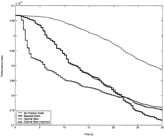
For the slewing mission, a baseball stitch trajectory with a frequency of 0.8 rad/s was chosen. The covector for this mission is dependent on the calibration method, but in general, the accelerometer errors and the gyroscope errors are evenly weighted. A per-formance index to compare the calibration methods is dependent on the covector and the covariance. The performance is independent of the position, velocity, and attitude of the vehicle since these are determined by the initial error prior to mission launch. The
performance index is ATPA for the states corresponding to the instrument errors. The performance of the four calibration methods is shown in Figure 6-9. As stated above, the performance requires calibration of both accelerometer and gyroscope errors. The six-position dwell is unable to calibrate rate-dependent gyroscope errors; therefore, this calibration technique and other inertially stabilized systems will not be competitive with inertially referenced slews. The final performance index for a six-position dwell is
3.87 x 10¹⁷.
The inertially referenced slews are able to calibrate the relevant errors for the inertially referenced mission. The baseball stitch performance is very good with a performance index of 3.75 x 10¹⁷, because it calibrates the same errors as those needed for the inertially
x c E AL 0-x 10 7 Time (s)
Figure 6-9: Performance Index versus Time given a Slewing Mission.
referenced slew mission. The optimal slew trajectory changes the angular velocity of the trajectory continuously and linearly after each measurement. The angular velocity is limited to ±0.8 rad/s to prevent gimbal lock. This optimal slew trajectory does not initially perform as well as the baseball stitch, but near the end of the calibration they are very similar with a performance index of 3.76 x 10¹⁷. The initial lack of improvement could be due to the necessity to move from one measurement axis to another, which has a higher correlation with the covector. Note that the baseball stitch and the optimal slewing trajectory have less improvement near the end of the calibration. The baseball stitch is observing the errors over a limited set of axes. The optimal slew trajectory reaches a local optimum, which has the maximum correlation between the measurement axis and covector. These limitations of the baseball stitch and optimal slew trajectory prevents future observability. An improvement to the optimal slew trajectory would be to move to another orientation to find another local optimum.
The improved optimal slew is identical to the optimal slew trajectory, except at 15 seconds the entire IMU is reoriented 90 degrees about the x-axis. The purpose of this reorientation is to create observability along another axis. As seen in Figure 6-9, this method is extremely successful with a final performance index of 3.72 x 10¹⁷. The optimal slew has the ability to find the maximum correlation between the covector and measure-ment axis. Once that correlation is determined, measuremeasure-ments will continue around a single axis. If another local/global optimum is along another axis, then the topology of the subspace may not have a path to find the other optimum. The improved optimal slew provides an escape from the local optimum. Rotating the IMU 90 degrees is arbi-trary. This improved optimal slew shows that escaping local optima needs to be further explored.
6.3 Inertially Stabilized Mission
The inertially stabilized mission requires calibration of primarily the accelerometer errors. The inertially stabilized mission has a nominal angular velocity of 0 throughout the en-tire mission without a reorientation of the IMU. This mission is very different than the slewing mission, because the rate-dependent gyroscope errors are insignificant. As shown from Section 6.1, the baseball stitch is not able to calibrate the accelerometer errors to the same accuracy as the six-position dwell. However, the optimal slewing trajectory is based on improving the correlation between the measurement axis and the covector. This simulation is to determine whether the optimal slewing trajectory can perform as well as an inertially stabilized mission.
Figure 6-10 determines that the best way to calibrate accelerometer errors is using an inertially stabilized calibration system. The performance index for the six-position dwell, baseball stitch trajectory, optimal slew trajectory, and improved optimal slewing
the IMU cannot improve the observability of the accelerometer errors to the accuracy of the six-position dwell calibration.
,2E
a-Time (s)
Figure 6-10: Performance Index versus Time given an Inertially Stabilized Mission.
Chapter 7
Conclusion
This thesis examined the inertially stabilized system and found that this is an ideal method for calibrating the accelerometer errors, but not the rate-dependent gyroscope errors. In order to calibrate the gyroscope and accelerometer errors, a new system, an inertially referenced slew, was considered. The inertially referenced slew calibration mechanization rotates the inertial measurement unit with respect to inertial space independent of vehicle motion. The advantage of using such a system is the ability to obtain gyroscope and
accelerometer observability.
In this thesis,, the covector measuring the downrange and crossrange miss for a partic-ular missile flight has been chosen as the performance index. In evaluating an inertially stabilized mission trajectory, the six-position dwell (an inertially stabilized calibration) performs the best. Slewing maneuvers were seen as a possible improvement strategy, but the six-position dwell is a far superior method for properly determining accelerometer errors during calibration.
Recent literature has proposed performing a slewing maneuver during the mission to improve accuracy. For this thesis, the baseball stitch slew was considered as a likely can-didate for the mission slewing maneuver. The baseball stitch slew has the property that during the mission it desensitizes errors, such as accelerometer bias. Since the mission
requires observability of the gyroscope and accelerometer errors, the six-position dwell calibration is not adequate in performing an accurate mission. The baseball stitch slew was considered to perform the calibration, since it will separate the errors improving observability. Also considered was an optimal slewing maneuver, which finds the opti-mal angular velocity to have the maximum correlation between the measurement and the covector. Maximizing the correlation directly relates to improving observability of the significant covector errors. The optimal slewing maneuver would often find a local minimum and not be able to traverse over a large set of angles. In order to improve the accelerometer observability, the inertial measurement unit was rotated 90 degrees about the x-axis half-way through calibration and the optimal slewing maneuver was repeated. This improved optimal slewing maneuver calibration performed the best for a baseball stitch mission trajectory.
These results validate the importance of having an appropriate calibration method for a given mission strategy. If the mission strategy focuses on accelerometer errors, then it is important to disassociate the accelerometer and gyroscope errors. Whereas, a mission strategy with accelerometer and gyroscope calibration requires excitation of both the specific force and angular velocity. In this case, it is important to implement a slewing maneuver, which observes the appropriate errors.
7.1 Future Research
For a given mission strategy, a calibration technique must be specified to improve the appropriate errors. Calibrating the entire inertial measurement unit requires maximum observability of both the gyroscopes and accelerometers. None of the calibration tech-niques in this thesis discuss maximum observability. A future area of research is deter-mining the ability to create maximum observability for all gyroscope and accelerometer errors. From the results of this thesis it appears that a combination of dwells and slews
must be performed. The problem must be restricted further to limit the infinite number of sequences and the infinite set of rotations to formulate a viable approach.
The reason for performing an inertially referenced slew is to desensitize the calibration procedure to certain errors. In the baseball stitch, this means desensitizing the calibration to accelerometer bias. If the baseball stitch is reversed, then one can desensitize it to gyroscope scale factor. This idea of desensitizing calibration is a dual problem, which can be seen as an anti-calibration. Eliminating specific errors from the calibration problem can improve observability of other errors. The success of desensitization has not been addressed in this thesis. The baseball stitch slew assumes improved observability by desensitizing the accelerometer bias, but this assumption has not been verified.
Another area of future research is improving the optimal slewing maneuver. The optimal slewing maneuver finds a local optimum by correlating the covector and the measurement. Using other heuristic optimization techniques, such as genetic algorithms, the global optimum could be found to improve observability. However, this may result in observability only along one axis of the inertial measurement unit. A global optimum search would be required at every time step in order to have maximum observability over the entire calibration period.
Appendix A
Quaternion Algebra
Quaternions can be written in the 1-3 form or
qO
where q is a 3-vector. Quaternion multiplication is defined as
pq [ qOPo - * P
poq + qoP + P x q
(A.1) (A.2)I
The set of unit quaternions satisfies q2 + Iq2 = 1. The result of quaternion multipli-cation of two unit quaternions is a unit quaternion.
The unit quaternion can be extended to an orthogonal linear transformation or rotation matrix R(q) where qO0 + q1- q2 - q3 2(qlq2 + qoq3) 2(qlq 3 - qOq2) 2(qlq2 - qoq3) qO2+ q22 + q2 _ q3 2(q2q3 + qoql) 2(qlq3 + qOq2) 2(q2q3 - qoql) q0 + q3 - - q2
The basic equation for rotation kinematics dependent on rotation matrices is R =
[Q x]R. The corresponding quaternion rotational kinematics diffential equation is
1 0
q= 2 q (A.4)
Appendix B
Initial Errors
position = 10 m velocity = 0.1 Irl/s attitude = 0.001 rad gyroscope misalignment = 5 x 10- 4gyroscope scale factor = 2 x 10- 4 gyroscope bias == 4.8 x 10- 7 rad/s gyroscope non-orthogonality = 5 x 10- 4
accelerometer misalignment = 5 x 10- 5 accelerometer scale factor = 1 x 10⁻⁵
accelerometer bias = 3 x 10- 4 m/s 2