Approximation of transfer functions by continued fraction expansion.

BY CONTINUED FRACTION EXPANSION

by

Charles Louy

B.Sc.A., Universite de Montreal (1971)

Submitted in partial fulfillment of the requirements for the degree of

Master of Science at the

Massachusetts Institute of Technology June, 1972

Signature of Author . . . .

Signature redacted

Department of Electrical Engineering, June 16, 1972

Signature redacted

Certified by . . . . . . . . . . .

Thesis Supervisor

Accepted by

Signature redacted...

Chairman, Departmental Committee on Graduate Students

Archives

NOV 15 1972

APPROXIMATION OF TRANSFER FUNCTIONS BY CONTINUED FRACTION EXPANSION

by Charles Louy

Submitted to the Department of Electrical Engineering on June 16, 1972 in partial fulfillment of the requirements

for the Degree of Master of Science.

ABSTRACT

This thesis deals with properties of the expansion of rational transfer functions into a continued fraction and their applications to the approximations of transfer functions by reduced order models. After a summary of known results, numerical examples are presented to compare different methods of approximation. A necessary condition for the stability of a transfer function is given in terms of the parameters of its continued fraction expansion. The effect of truncating a continued fraction on its Taylor series expansion is studied and an explicit perturbation formula is developed. This then yields an algorithm to realize a transfer function from a finite number of terms of its Taylor series expansion. The derivation

includes a simple analytical expression for the inverse of a particular state matrix associated with the transfer function.

Thesis Supervisor: Jan C. Willems

ACKNOWLEDGMENT S

It has been a pleasure to work under the supervision of Professor J.C. Willems to whom I am particularly grateful. I am indebted to Dieter Willner for his numerous criticisms and especially for moral support. I would like to thank also Philippe Coueignoux with whom I had fruitful discussions. The typing by Mrs. Karolyi is indeed appreciated.

4 TABLE OF CONTENTS Page ABSTRACT . . . . . . . . . . . . . . . . . . . . . . . . . . . ACKNOWLEDGMENT . . . . . . . . . . . . . . . . . . . . . . . . CHAPTER I INTRODUCTION . . . . . . . . . . . . . . . . . . I-1 Structure of the Thesis . . . . . . . . . . . . .

CHAPTER II CONTINUED FRACTION EXPANSION . . . . . . . . . . II-1 Continued Fraction Expansion for Passive Networks 11-2 Analysis from the Control Viewpoint . . . . . . . 11-3 State-space Formulation . . . . . . . . . . . . . 11-4 Expansion by Routh's Algorithm . . . . . . . . .

2 3 . 6 . 8 . 9 9 . 11 . 15 . 16

CHAPTER III COMPARISON WITH OTHER METHODS . . . . . . . . . III-1 Reduction by Diagonal-Element Discarding [1-5] 111-2 Reduction by Pade Approximation . . . . . . . . 111-3 Example [9] . . . . . . . . . . . . . . . . . . 111-3.1 Second Order Approximation . . . . . . . . . 111-3.2 First Order Approximation . . . . . . . . . . 111-4 Conclusion . . . . . . . . . . . . . . . . . . CHAPTER IV NEW RESULTS . . . . . . . . .

IV-1 Stability Test . . . . . . . IV-1.1 Necessary Condition . . . . IV-1.2 Example . . . . . .. ... IV-2 Frequency Analysis . . . . . IV-2.1 Taylor Series Expansion . . IV-3 Realization Algorithm . . . . IV-3.1 Computation of rp . . . . . CHAPTER V CONCLUSION . . . . . . . . . . .

Suggestions for Further Research APPENDIX DERIVATION OF A. . . . . . . . .

A-1 Computation of the Determinant . A-2 Cofactor of a Diagonal Element Eii

A-3 Cofactor of an Upper or Lower Diagonal Element A-4 Cofactor of the Other Elements

REFERENCES . . . . . . . . . . . . . . . . . . . . . . . . . . . 21 . . 21 . . 23 . . 24 . . 24 . . 26 . . 28 . . . . . . . . . . . 29 . . . . . . . . . . . 29 . . . . . . . . . . . 31 . . . . . . . . . . . 32 . . . . . . . . . . . 34 . . . . . . . . . . . 37 . . . . . . . . . . . 40 . . . . . . . . . . . 4 1 . . . . . . . . . 44 . . . . . . . . . 45 . . . . . . . . . 47 . . . . . . . . . 47 . . . . . . . . 49 51 53 55

LIST OF FIGURES

Fig. Page

Number

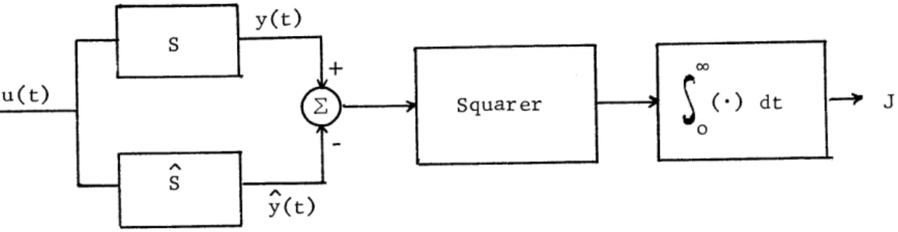
1 Criterion of performance: minimization of J 7 2 Continued Fraction Expansion for Passive Networks 10

3 Block Diagram Representation of (6) 11

4 Block Diagram Representation of a General Continued

Fraction 12

5 Second Order Simplified Model 14

LIST OF TABLES Table

Number

6

Chapter I INTRODUCTION

The transfer function of a system is usually obtained experi-mentally or from the transfer function of each individual component of the system. In most industrial applications it is not feasible to deduce a mathematical model from first principles. Therefore most practical methods of deriving a mathematical model make use of ex-ternally observed data, the input-output description. In many cases we thus obtain a large set of time-invariant differential equations. Reducing the order of a transfer function or decreasing the dimension of a state matrix is highly desirable or sometimes necessary in the analysis and design of a control system. This is due to the fact that essentially all design methods yield a system (i.e. a dynamic compen-sator) whose complexity is directly proportional to the order of the original system. The computational effort to obtain this design is usually proportional to a power of the order of the original system.

Given a transfer function, we would like to find approximating transfer functions of lower order such that the outputs of the two systems are as close as possible when the same input is applied. Obviously this choice depends on the criterion of goodness we choose. For instance, one may want to minimize the integral of the square of the difference between the outputs of the two systems (see Fig. 1). Theoretically this approach is always possible. But, as we will show

S y (t)

u(t) Squarer dt -> J

0

y(t)

Fig. 1: Criterion of performance: minimization of J

in a very simple example, it leads to complicated computations which are not practical even in the simplest cases.

The general techniques presented in the literature correspond to approximating a system by its dominant poles and zeroes in the complex plane. This is the main idea used by Davison and Chidambara [1-5]. However, many systems have no "dominant" roots and the con-ceptual basis of such a technique is at best unclear.

In an article published in 1970, Chen and Shieh [6] presented a novel method for simplifying the transfer function or the state matrix of a control system. In the frequency domain the transfer function is expanded into a continued fraction which is truncated according to the degree of the reduced model we want to obtain. This method is very attractive for the following reasons:

1) The quotients (hi, i = 1,...,2n) of the continued fraction expansion can be computed by a very simple algorithm.

8

2) These quotients have a direct physical meaning in terms of feedback control and it is easy ,o write a state variable representation of the transfer function where the matrices A, B, C are function of the hils. In this state variable form the reduction technique cor-responds to discarding rows and columns of the matrices A, B, C.

I-1 Structure of the thesis

In Chapter II we will summarize the results related to the con-tinued fraction expansion. Chapter III includes numerical examples in order to compare different methods of model reduction. In chapter IV, we will present new results, with respect to Chen's method, which will lead to a partial realization recursive algorithm.

Chapter II

CONTINUED FRACTION EXPANSION

The theory of continued fractions is not recent. It is a power-ful tool to perform numerical analysis by hand. A complete theoretical treatise can be found in Wall [7] and Khovanskii [8], the latter empha-sizing numerical analysis aspects.

II-1

Continued fractions have been used extensively in network synthesis. The driving-point impedance of an RC network can be written as a ratio of two polynomials with real negative roots. It is well known that this rational function can be expanded in the so-called Cauer form (see ref. 10, p. 119). Zn(s) = bo+bls+---+b 2 s -2+bn- 1s " ao+as+-- .+an-₁s 1+ sn h, + ₁ ha 1 s2 +y+ h3 + h4e sS

where the hit s are all positive and represent the inverse of resistances and capacitances as shown in Fig. 2. The hi's may be obtained by or-dering the two polynomials in ascending order with respect to the

10

1 1/h 4

1 1 A 4

h, h 3 h2n-1 han

Fig. 2

powers of s and by performing successive divisions. Therefore h, is equal to the ratio of the constant terms ao/bo.

If we look at the circuit of Fig. 2, we see that the value of

the impedance for u = const. (i.e., D.C. input) is

z(0)

=

(2)

whereas for an infinite frequency the circuit behaves as the series connection of all the capacitors

lim Z(jOw) = lim . (3)

o -+ 00 -+ oo

If we take the limit of the rational fraction (1), we obtain

bn.1 lim Z(jo) = lim

W -+- 00 W --- COo

d

Comparing (3) and (4), we can state heuristically that

bn _1 = t h=2k k =1 Z (s)

(4)

We see, intuitively, that the low frequency response of the circuit is affected only by the elements nearby the input in Fig. 2, in other words only by the hits for which i is small. So, if we truncate the

con-tinued fraction and keep only the first 2m quotients (where m < n) we might expect that the resulting new function is a low-frequency ap-proximation of the original impedance. In Chapter IV, we will prove rigorously that this is indeed the case for a general continued fraction.

11-2 Analysis from the Control Viewpoint

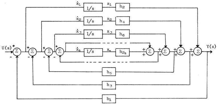
Chen and Shieh [6] have extended the approximation method outlined in the previous section to general systems. The transfer function is expanded into a continued fraction as in Eq. (1). Since we cannot re-present a general system as the RC network of Figure 2, some of the hi's may be negative. Yet it is possible to give a physical

interpre-tation of the continued fraction in terms of feedback control. Consider the transfer function given by

h2 s -+ Gl(s) Y(s) 1s ₍₆₎ Uh ₁ + h U~s) _{h, + + h,} --2+ Gl(s) -- + Gl(s) S

It can be represented by the block-diagram of Fig. 3.

-+h2/sI

Figure 3

U(s) + " Y(s) Fgr

YsG)(s) Block Diagram Representation of (6)

1/ s

.

...

1=hs

U Y(S)

Fig. 4. Block Diagram Representation of a General Continued Fraction. The xi's are used in the state variable representation of the system.

If G,(s) = 1 (7) 1 h- + 3 h2 - + G₂(s)

we can draw a block-diagram for Gl(s) itself as in Fig. 3.

We are now able to represent the general continued fraction

Y(s) 1 ₍₈₎ U(s) h2 1 ss ha + h4 1 S h₂n

by the scheme of Fig.

4.

U(s) + t + Y(s)

[LEZ

11-3 State-space Formulation

The reduction technique is interesting when we convert it into a state-space formulation

x = -A x + B u y c x

In Fig. 4 we may choose the output of each integrator as a state variable xi. Then we obtain

~xi7

K

From (10) we note the following:

1) the elements in the state matrix are simple, combinations of the quotients obtained from the continued fraction;

2) the elements appearing in a position lower than the diagonal have the same value as the diagonal elements above them;

3) the elements in the upper triangle are expressed in terms of quotients in a very regular way.

16

These special features will be exploited in Chapter IV.

In this state variable representation the reduced models are ob-tained by matrix partition. For instance, if a second order reduced model is desired, we simply take the upper left-hand corner of the original matrix as the reduced one. That is:

x-1

[]=

h

-+

II-4

This section presents an algorithm due to Wall [7] which expands a rational function into a continued fraction. We change the notation of the coefficients of (1) using double subscripts as follows:

G(s) = R2 1 + R2 2 s + R23 S2 + + R2 ,, sn~ (12) R₁₁ + R1 2 s + R, 3 s2 + - + R1, s ~1 + s5

Performing the division on (12), we obtain

G(s) = 1 (13) (R2 1RI2 - R1 1R2 2) (R2 1R, - -RIR2 Z) 2 R11 R21 R2 1 R2 1 R21 + R2 2 s + R23 S2 +- - -+ R2, n s n~ We define R_{2 1}R_{1 2} - RIR22 = R 21(1) R2 1

and R21R,3 - R_{1 1}R₂3 R2 1 R32 Equation (13) becomes G(s) = R1, R31s + Rs2 + + 2s R21 R21 + R2 2S + R23S2 + .

Continuing the division, we have

G(s) = R, 1 R21 + R_{2 1} 1 R_{2 2}R - R R2 1 R_1 s +-R- + R32 s + -Define again R_{2 2}RM - Rs2R_{2 1} = R. Ra etc.

Finally we have the expansion 1 G(s) = R₂₁ (19) R R21 5 S R_{4 1}

which can be written alternatively

(15)

(16)

(17)

18

G(s) = 1 (20)

R41

Comparing eqs. (20) and (1), we have

h, = R (21)

with the general recursive algorithm

Rik = Rj-2,k+1

-Rj.., , j = .34, 5 ... 2n+1 (22)

1,2,3 ... 2 for

j

1,2,3 ... for j even

Therefore we write the coefficients of the denominator and the coefficients of the numerator of the transfer function as the first and second row respectively of an array. The other coefficients are obtained in the same way as those in the well-known Routh's array for verifying whether or not a polynomial has right half plane zeroes. This algorithm is very suited for automatic computations.

11-5 Example

As an illustration, consider the following transfer function

s 360 + 171s + 1052

G(s) = (23)

720 + 702s + 71s2 + s3 A continued fraction like (1) is desired.

. Write the first and second rows of the Routh's array by copying

the coefficients of the denominator and the numerator respectively, and then use eq. (22) to generate lower rows

720 702 71 1 360 171 10 360 51 1 (24) 120 9 24

4

The h 's are than found by taking the ratio of the neighboring terms of the first column

h = R,, PR , h= 2 h₂ = 1 h = 3 h4 = 5 h5 = 6 h₆ =

4

20

from which the continued fraction is written as follows:

G(s) = (25) 2 + s 1+ 3 + s 5 + s 6 +

Chapter III

COMPARISON WITH OTHER METHODS

In this chapter we are presenting numerical results to compare different existing methods of model simplification. Here is a brief description of the techniques.

III-1 Reduction by Diagonal-Element Discarding [1-5] Suppose the initial system is given by eqs. (26)

k = A x + B u (26)

where x is an n-dimensional vector. The eigenvalues of the A matrix have negative real part and we index them in order of increasing moduli

L~l<

Suppose, furthermore, that it is possible to distinguish two groups n...dm)

and ( ...

A)

Define by M the matrix of the similarity transformation which puts A in diagonal form. (Note that we assume distinct eigenvalues for A.)

x= Mz ==> =A z + G u with

A = _?' A M = diag (h, ... h,) G =M' B

22

We partition the matrices as follows

AL . 2 A, = diag(\, ... Am); A2 = diag(\m+i...?\)

Al

L_ 3 A4 L3 M4 x=K I1 = j

We want to approximate the system described by eq. (26) by the system

= A* x + B* u (27)

We choose A* (m X m)such that x* is a good approximation of the first m component of the vector x.

The transformation x = M z implies that:

j = Al zi + GI u

2 = A2 z2 + G2 U

with xI = M1 zI + M2 z2

x2 = M- zi + M4 Z2

Chidambara applies the following idea: The modes of

Amei

X2 = M- N1 x₁ - (M4 - M, M' M2) G2 U (28) The model used by Davison is defined by

= (A, + A2 M3 Mi)xi + M1 GI u

-1

X2 = -3 MI xI (29)

Eq. (29) is a consequence of eq. (28) if we assume that the

eigen-value of A2 go to infinity.

111-2 Reduction by Pade Approximation

Recently Hsia [9] has developed the following procedure. We are given the high-order system described by the transfer function

1 + als + a2s + ''. + amsm

H(s) = K m< n

1 + bIs + b₂s 2+ ... + bnsn

which we want to approximate by the lower order function

L(s) = K p < q < n

1+ djs + - -+ d s

The idea is very simple. Develop both IH(jw)12 and L(j)12 in a Taylor's series around w = 0 and set the coefficients of the same powers of w to be identical. This will lead to (p+ q) nonlinear

equations in the unknown parameters of L(s).

It is important to note that since there are no constraints on the poles of the reduced system, Hsia's method as well as Chen's may yield unstable models. In Chapter IV, we will give a necessary con-dition for the stability of Chen's reduced models. On the other side,

24

the following numerical example shows that Hsia's and Chen's methods can end with a better result than the dominant pole-zero philosophy.

111-3 Example [9]

We want to reduce the following fourth order transfer function

G(s) = s3 + 7S2 + 24s + 24 (30)

s4 + l0s3 + 35s2 + 50s + 24

111-3.1 Second Order Approximation

The second order continued fraction expansion gives hi = 1

h2 = 0.92308

h: = -14.0833 h4 = -1.9264

This yields the following transfer function

G2(s) - -1.00332s + 25.04308 _ -1.00332s + 25.04308 (31)

S2 + 26.12675s + 25.04308 (s + 0.9965)(s + 25.1301)

As we pointed out in Chapter I, we must select a numerical cri-terion in order to compare different results. In the following Table I we denote by J- the integral of the error squared in the unit step response and by Jo the integral of the error squared in the impulse response.

Transfer function Unit step response

y(t) = step response of original system

y(t) = step response of reduced system e(t) = y(t) - y(t)

J =

s

dt ; J0 =

50

de (t) 2 dt

dt t

Model Remarks J-₁ Jo

. . s3+7s2+24s+24 y(t)= ₁-e-t -2t exact step 00

Original system 2-3t -4t response

(fourth order) s4+l0s3+35s 2+50s+24 +2e - e

0.8333s + 2 7 -t 1 -2t second order 0.00033 0.00304

sia-1 3s + 2 1 - e + e models with

two prefixed Davison 1.0833s + 2 -t -2t poles at -1 0.00693 0.01624 2 + 2 12 12 and -2 s5 + 3s +2 Chidambara 0.5833s + 2 1 -t 1 -2t 0.01144 0.05489 s2 + 3s + 2 6

Chen -l.00332s+25.04308 1 -1.0829 e-0.9965t second order 0.00107 0.08225 (s+0.9965)(s+25.1301) -25.1301t models with +0.08286 e unconstrained -2.4t poles Hsia-2 0.2917s + 1 1 - 0.2308-.4t 0.00012 0.2459 0.399s2 + 1.375s + 1 -1.2308 e-li043t U-1

26

A brief comment on the results: Let us classify the different methods in order of increasing error. With respect to J- we obtain:

Hsia-2

<

<

<

<

Hsia-1

<

<

<

<

This shows how heavily the performance of a method depends on the criterion we choose. In particular, Hsia-2 is the best result with respect to the unit step response error Ja and, at the same time, the worst result if we choose the impulse response error Jo as the cost.

111-3.2 First Order Approximation

For the first order model Chen's method and Hsia's give the same result

Transfer function

Unit step response Error (as defined in

Table I)

G1 (s) 0.923 s + 0.923 y(t) = 1 - e-O.923t

J-1 = 0.00105

We are going to show that this result is not optimal with respect to J-. To do so let us look for the unit step response

Y1(t) = 1 - p e (32)

where p and q are to be determined so that J1 is minimized. The exact

y(t) = 1 - e-t - e-2 + 2e~3 - e-4t

The difference squared of the responses is defined as

e2 (t) = (p e~ t - e-t - e-2t + 2e~3- e-4t ) (33) Developing the square and integrating we obtain:

J. = e2(t)dt =2- 2p 2p + -2

SSe d 2q q+1 q+2 q+ 3

0 ₍₃₄₎

+2 2 4 +7

Necessary condition to minimize J-1 are :

F~II-P

6p q q +1 q + 2 q + 3 q + 2

_ ')+ 2p + 2p 4p + 2p (36)

)q 2q2 (q+l) (q+2)2 (q+3)2 (q+4)2

From eq. (35) we can write

2 2 4 +

q-

q + 1 q + 2 ~q + 3 +q + 4(7

Equation (36) yields p = 0 as one of the solutions. This implies that e = 0.57. Therefore p = 0 is not optimal since we already have a better solution. We can divide (36) by p to obtain

- + 2 2

4

2q2 (q+1) 2 (q+2) 2 (q+3) 2 (q+4) 2 Using (37) into (38) leads (after some algebra) to (39)

q7 + 17q6 + 125q5 + 457q4 + 762q-3 + 250q2 - 716q - 624= 0 (39)

28

Equation (39) has only one positive real root which is therefore the optimal we are looking for:

q* = 0.9353

Using eq. (37), we obtain the optimal value for p

p= 1.032

From eqs.(35) and (34) the optimal cost can be written as

= *2 +2 2 24 7

J =2q+ 3 - 5 - + 8 = 0.00068

2q* 3 57 8

This represents a reduction of 35%0 on the cost of Chen's method.

III-4 Conclusion

Two ideas have been developed in this chapter. We cannot say that one method is better than the other one since the performance depends on the input we apply to compare the outputs of the two

systems. Once we have chosen a cost criterion, we can theoretically find the optimal transfer function but this involves a great effort in computation. Among all the methods presented, Chen's is the one which

Chapter IV

NEW RESULTS

This chapter deals with two major issues concerning the approxi-mation of a transfer function by truncation of its continued fraction expansion. First, we want to present a test for the stability of the reduced models. In the second part, we are going to investigate the nature of the approximation in the frequency domain and its

conse-quences.

IV-1 Stability Test

A major inconvenience with Chen's method is that it may yield unstable reduced models even when the original unreduced model is

stable. For instance, given the second order minimum phase transfer function G₂ (s) 2 + 3s

(40)

~1

2

.4

The first order approximation is given by

Gl(s) (41)

Clearly G2 (s) is stable but Gl(s) is unstable. Since Chen's method

30

to find an easy test to check the stability of the reduced models. Given the parameters hi (i = 1,...,2m) we can find the coef-ficients of the corresponding transfer function through the inverse of the Routh's algorithm. With the same notation of Chapter II,

the Routh array may be written in the following form

R11 R1 2 R,- R14 ... Ri,m I h, R2 1 R2 2 R2 Z R24 ... R2,rM h2 1 R RZ2 R33 R34 ... 1 (42) R2mi ham

We have assumed that the denominator of the transfer function is a monic polynomial. Therefore

j2m

-j

' 2 = 1; j = 1,3,5,..., 2m+1 (43)

The first column of (42) can be found by inspection

R2m,1 = h2m R2m-l,l = R2m,j h2m,- = h2m h2m-1 2m R j,1 = Rj 1,1 hj = IT hi 2m R2 1 = ao = RZ1 h2 = H hi i=2 R1 1 = bo=R2 1 h,= HT hi (44) i _1

We then proceed to compute the second column, the third, etc., by applying the reverse manipulations from those which lead to (22)

Rj-2 k+l = Rik + R-2₁ Rj-1 (45) Or more simply

Rj-2 k+1 = Rik + hj-2 Rj-1,+k1 ; (46)

j = 2(m-k)+3,... ,5,4,3

RJ is known because we compute the kth column before the (k+l)th. The coefficient Rj-1,,Ui is also known since we compute the elements of each column starting from the bottom.

Once we obtain the coefficients of the characteristic polynomial (the first row of the Routh array) we can easily verify the stability of the transfer function.

IV-l.1 Necessary Condition

The following remark will lead to a simple necessary condition on the h parameters for the stability of the transfer function.

From eq. (44), we know that when the coefficient of the highest power of s of the characteristic polynomial is equal to 1 then the constant term is given by

2 m

bo = R,= 11 hi

i=1

But a necessary condition for all the roots of a polynomial to have negative real part is that all its coefficients have the same sign. This implies that the product of all the hi's must be positive in order for the transfer function to be stable. We can therefore state the following

32

Theorem 1: Given a transfer function, a necessary condition for its stability is that all the coefficients hi's of its continued fraction expansion (1) be positive or an even number of hi's to be negative.

With Theorem 1 in mind we could have stated immediately that the first order approximation of (40) is unstable because hjh2 =

- < 0.

Important remark: It follows from Theorem I that a necessary and sufficient condition for the stability of all the reduced models is that all the hi's be positive. This corresponds to asking G(s) to be the driving point impedance of a RC network, i.e. G(s) has the pole-zero pattern

N - w

and its impulse response is i-e , t > 0, with > 0 and

0

Ai > 0.

IV-1.2 Example

Suppose a reduced model is described by 1

h1 , h

.12-l, h3 2~ h4=4

R1 1 R12 R2 2

R2 1 R2 2

h₂

R31 R32

R₅₁

We compute the elements R5 =

1

4

in the following order assumption) -2 2 2 = 1 (by assumption) = h4 + h2 = 3 = R_₁ + hjR_{2 2} = 1 R13 = 1 (by assumption) We obtain the 2 2 -2 4 1 following array 1 1 3 1

34

The corresponding transfer function is

G2(s) 2+ 3s

2+ s+s which is clearly stable.

IV-2 Frequency Analysis

In this section we want to estimate the effect of the approxi-mation using frequency domain techniques. Let us expand the

trans-fer function in a Taylor's series around s = 0. We know that the system is described by the following state equations

x = -A x + B u

y = C x

where A, B and C are given in Chapter II (10). The transfer function can be written as

f(s) = C (I s + A)' B = sl f(i)() (46)

j=0 l' s=0

The derivatives of f(s) at s = 0 can be obtained easily and are given by:

f(o) = C A B

f'(s) = C(I s + A)' I(I s + A)' B => f'(o) = C(Ai')2 B

f"(s) 2C(Is+A)-' I(Is+A)' I(Is+A)-' B => f"(o) =2C(A) 3 B

f (n)(s) = n! C(A)n B (47)

Therefore the general Taylor expansion formula around s = 0 is

(48) f (s) C(Is + A)' B =Z C(A)n+' B s"

n=O

We see that we will get additional insight if we find an analytical formula for A' To do this, it is useful to note that A may be factorized in the following form

h, ... hl+h3 h+h3 hl+h3+hs hl+h 3 h,+h 3+h₅ ... h,+hs+h5 -... h+h 3+...+h-1 Fh2 0 . hen (49) The inverse of A may then be computed as:

0 hF

I--L"

Performing the multiplication we obtain h, 1 1 AT = h1 0

36

1

+1 1 )

1

1

1

1

1

It is interesting to note that when we delete the last row and the last column of A for model reduction, the inverse of the new matrix is obtained from the old inverse by deleting also the last row and the

last column and letting 1 be equal to zero. A second interesting

h2n -1

property is that the sum of the elements of each row of A- is equal to zero except for the first one. As we expected, we find that the first term of the Taylor's series expansion of the continued fraction is

f(o) = C A B = (52)

h2

Looking at the structure of A one might suspect that C(A ) B is just a function of h, and h2 and that in general C(A)i B

gi(hl,...,hi) for any integer i.. We will now prove this statement by induction.

IV-2.1 Taylor's Series Expansion Consider the continued fraction

hi + h2 +

+ -s

(53)

Suppose f, has the following Taylor's series expansion around s =

0:

f (hl,...,hp s) = gj(hj)+ g2 (hl,h2)s+ -- + gi(h1,.

+ gp (h1,.. .,h,)sP ~+r (h1,...,hp)sP

+ O(U9) we want to prove that

f+,, (hl,...,h ,hp1,s) = h, + 1 (55) s h2 + s '+ s + S

has the following Taylor's series expansion

+1 (hi,...,hh,.,s) = g,(hj) +g92(hihj)+s + + gi(h,. . , h )si~1

+ r +I(h,...,hp+,)s-Pl + 0(sP+1)

(54) fp (h, Y. ... ,hp ,s) = :

... + g,(hl.,....,h,)s? ~l+ g,+.j(hj,...,hP41)sP

38

To do this, note that f,1 is equal to fp where we replace h, by

H, (s) = li + s We can therefore write

- + gi(hl,,... + gV (h , . H (s) sp + O(sp ) (57) ,hi)si~1+.-~1+ r, (h, .. , (s))sP (58)

Now develop g, (hj, . . . H, (s)) and rp (hI, ... , HP (s)) in Taylor ' s series

6H, (s) 6s + g, (h, .. .h ) 6h, + O(s) s (59) 6H, (s) 6s + r (hl,..h ) )N, + O(s) S (60)

Using eqs. (59) and (60) in (58) and noting that

OH,(s)

as

we obtain eq. (56) where

1

+ r, (h1, g+1 (hl,..

We have thus proved that the assumption of (54) implies (56). (54) is true for ff _{) istruefor}

_l

-hi, (61) (62) Since f +(hl, . .. ,hp~l, s)= g(hi)+ g2(hi~h2)+ -6gp (hj,.,h) .,h ) =p

Therefore the truncation of all the quotients hi (i > k) of a continued fraction is a low frequency approximation since the first k coefficients of its Taylor's series expansion around s = 0 are not affected by this truncation. This is a result we mentioned intuitively in Chapter II. If we denote a continued fraction (53) with n quotients hl,.. .,h by f,(h,.-..,h,,s) we can state the previous result formally:

Theorem 2: Given the two continued fractions f,(hi,...,h,s) and fm(hi,.. .,hm,s) with m < n, then the first m terms of their Taylor's series expansion around s = 0 are identical.

Let us find a more explicit formula for (62). Write (62) for

6gp -1 (hj.,...,h 1

gp (hi, ... , h) bh, -1 -+ r,-(h,.,hp _j)

(63) Now take the derivative of (63) with respect to hp and substitute

it in (62). This yields

1 -1(h,_ ... ,h, -_1)

gei i,.,hv+₁) = - 2

hp. h, 1h

h-+ r,(hl,..hp) (64)

Continuing the same procedure and recalling that

gj(hj) = - (65)

h, yield the general formula

40

gp+i(h,.. . h,]) + rp (hl, .,hi (66)

h+ _II hT i=1

Therefore, when we add one quotient to the continued fraction f,, the first p coefficients of its Taylor's series around s = 0 remain unchanged and the coefficient of sP is modified by (66). But now it is very easy to obtain the h parameters of the continued

fraction from the coefficients of its Taylor series.

IV-3 Realization Algorithm

We are given the coefficients gi (i = 1,2,...) of a Taylor's series around s = 0 and we want to compute the quotients of a continued fraction which will match these coefficients. We proceed as follows

= 1 From eq. (66) =2 h₂ r-g=- ₂ 2 2 h₂h, _g 2hi

Now we compute the coefficient r2 of s 2

in the Taylor series expansion of s . The general formula for r. is derived in Section IV-3.1.

h, +

-h2

Write eq. (66) for p = 2

(-l) (-1)

g= ( + r2 > h -=

h h2 h2 h2 h1 (g2 -r2)h2 h2(g ) 1 h2

Step 1 h, = 1 (g, - r0)k 2 k +- -kX h Compute r, Step 2 h2 = 1 (g2 - rl)k 2 k -- -k x h2 Compute r₂ Step p h, =-(g, -r _k k +- k X h Compute rp IV-3.1 Computation of rp From eq. (48) p = 1,2, ... where (67) (68) C = [h, h2 ...h2 i] 1 1 1 AI~ ~ N' = R 2 for p even for p odd 1, 1-h₂ ' -1 hai

where E can be deduced from eq. (50). r. = C(A )P+l B

42

We may therefore write

r, = C(A')V*l B = [1

(69)

It remains to define E' and A at each step. This can indeed be done by inspection of eqs. (50) and (51).

1) General odd step 2i-1 Calculate h₂ i-1 Define

,e

-ha -1

The new dimensions of E ' and A is i X i.

Denote by e,1 and a the general elements of E' and A respectively.

If i = 1 go to (72) If i = 2 go to (71) Set

eij., eji, ai, aji equal to zero for

j

6- ei- + '91

-

ej,

A

h2i-2 (70) ei- j -e j., i -1 ei-i, i air -(where 92 (71) A Iti E '(A ) P I i,1

egi

-(72)

ai+-

0

Now compute r_2i-1 according to eq. (69)

r₂ .. = 1 Er (A1 )2p ~1

2) General even step 2i

1 1

Compute h₂1 ' 2 h27

E' and A have still dimension i X i E1 does not change

aj.,i-1 <-- -agi r2p = 11 :- E'(A-') 2P

E -

-J 2

The algorithm is complete. The most important feature is its recursiveness. _{If we want to match one more coefficient in the Taylor}

series we simply have to go through one additional step in the recursion.

44

Chapter 5

CONCLUSION

The continued fraction expansion has revealed several interesting properties.

In approximation theory we emphasized that the performance of the reduced models depends on

1) the choice of a cost criterion;

2) _{the input applied to the systems in order to compute the cost.} The error minimization techniques have the advantage to give the optimal result with respect to a chosen criterion, and furthermore to preserve stability. On the other hand, these techniques lead to very involved computations. Therefore, these methods are not practical

since the aim of using these approximations often is to save

com-putational effort in the first place. In this respect, Chen's method has has the great advantage of simplicity. A more important feature is

the physical interpretation of a continued fraction in terms of feed-back control. _{This allows an immediate simulation of the reduced}

models. _{The analysis from the control viewpoint yields a direct} state-variable formulation from the quotients of the continued fraction. In Chapter IV we derived a remarkable analytical expression (51) for the inverse of the state matrix A. _{On the other side, we have obtained a} simple interpretation of Chen's approximation method in the frequency domain with the explicit perturbation formula (66) on the coefficients

of the Taylor series expansion of the continued fraction. These two results, eqs. (51) and (66), lead in a natural way to the recursive realization algorithm of Section IV-3.

SUGGESTIONS FOR FURTHER RESEARCH

In Section IV-1, we obtained a simple necessary condition for the stability of a transfer function, namely that its continued

fraction expansion must have an even number (including zero) of nega-tive quotients. This result was found in computing the constant term bo of the characteristic polynomial through the inverse of the Routh's algorithm. It might be possible to find stronger conditions on the h parameters of the continued fraction by considering the expressions of the other coefficients bi. To be explicit, consider the Routh array of a second order transfer function

h, h h3 h4 h3 h4 + hj(h2 + h4) 1 h2 h3 h4 h4 + h2 h - h4 h₄ 1 We obtain bo = h, h2 h3 h4 b, = h3 h4 + h, h2 + h, h4 b₂ = 1 (by assumption)

46

The idea is to find stability conditions on the hi's. The main dif-ficulty is that the hi's depend also on the coefficients ai's of the numerator of the transfer function whereas the stability con-ditions are independent of the ai's. It should be kept in mind

also that the conditions to find should be simpler than the stability test which computes the bits through the inverse Routh's algorithm. Sufficient stability conditions could be useful too.

Another interesting area of investigation is the approximation of an irrational transfer function through the truncation of its con-tinued fraction expansion. Khovanskii [8] devotes several chapters to this matter.

Finally, it would be of interest to extend the results of Chapter IV to multi-input multi-output linear systems.

Appendix DERIVATION OF A

Given the (n X n) A matrix as factored in eq. (49) An = En diag(h₂, h4,...hen)

where En is the (n X n) matrix defined by

el el el el ... el ... e2 .. en el e2 e3 e el e2 e2 e2 (A-1) (A-2) n and ej =

D

We want to find An = diag , ,..., E . The main task is - h2 h4 "

han-to find En

A-1 Computation of the Determinant We have det E, = el el det E2 = el el = el(e2 -

el)

Let us express det E, as a function of det En. For clarity in the next arrays we will not write the letter e but only the subscript. In other words i stands for ej.

det E,+₁ = 1 1 1 2 2 1 2 3 1 1 2 2 3 n-1 n-I n-I 1 2 3 ... n-1 n n 1 2 3 ... n-1 n n+1

Note in (A-4) that the nth column and the (n+1) column are identical down to the nth row. Therefore

det E,+ = e,+, det E. - _{e. det En = (e,+ - e,)det E.} We have thus obtained the recursive formula

det En = ej(e₂ - ej)(e3 - e2) .. (en - en-1)

₍

Using (A-3), this becomes

n

det En = 11 h2

i

(

i =1

Note that

2n

det An = II hi = RI, = b0 = constant term of the denominator

of the corresponding transfer

A-5) A-6) A-7) function 48 3 (A-4) 1 (A-8)

A-2 Cofactor 1 1 1 1 1 1 1

of a Diagonal Element Eii

... i-i ... i-i ... i-i ... i-i i-i I I I i-1i i+1 i+1 i-I i+1 i+2 1 2 3 ... i-1 n-2 n-2 i i+1 i+2 ... n-2

Let us denote by Eij the general element of E. From (A-9) we see that the cofactor of E₁₁ is the determinant of the (n-1) X (n-1) matrix obtained from E, by discarding the first row and the first column. It is therefore equal to det En-, where we add one to all the indices. Thus,

cof(Ell) =

cU

i)(G3

cn-1)

Therefore

cof (Ell)

det E, _{el (e2 -}e2 _el) ,

2 3 (A-9) n-2 n-1 n-1 n-2 n-1 n V n (A-ll)

50 In general the cofactor of Eri is equal to the determinant of E"-1

where el, e2,....,ei-, do not change, but we add 1 to the index of

ej for

j

cof(Eii) = ej(e2-e1). ... (ei-I -ei- 2)(ej+i -ei-1)(ei+ 2 - ei+i)

... (e. - e.-₁ ) (A12)

Recall that

det En = ej(e2 -el)...(ei-1 - ej-2)(ei - ej-1)

(e +j - e)

.

.-

Dividing (A-12) by (A-13) we obtain

cof(E i) det [E]n

ei+i- ei-I

(ei - ej -1) (ei+ j - ei) (A-14)

Using (A-3) into (A-14) yields

cof(E i) h₂i+1 + h2 3 11

=+ _(A-15)

h2 i-I h2 i+1

If we define ej = 0 for

j

j

A-3 Cofactor of an Upper or Lower Diagonal Element Ej ,1j= E+1 , Previous remarks:

a) Given En, the nth row differs from the (n-I)th row by the element E,, only. This implies that

b) If we cancel the last column of E,, the last two rows of the resulting matrix will be equal.

In order to compute the cofactor of Ej i,, we cancel the ith row and the (i+l)th column of En and compute the determinant of the resulting matrix (and change the sign of the result). At this point we have two cases:

1) i = n-1

In this case the resulting matrix is obtained from En by cancel-ling the nth column and the (n-1)th row. But by remark b) above, once we have deleted column n, the nth row and the (n-1)th row are

equal. So that the resulting matrix in question is equal to the matrix we obtain from E, by deleting the last column and the last row. But

this is exactly En-1. Consequently,

cof(En-1 ,n) = -det En-i (A-18)

Therefore

cof(En-, n) 1 1

(A-19) det En e. - e.-i

h2n-2) i/n-1

52

determinant of the resulting matrix G A E" (i, i+1)." Let us compute the determinant by expanding the last column

G21 = eiG(1,n)1 - e2fG(2,n) + ... + ei-1G(i-1,n)f + ej+₁jG(i+1,n)f + --- + en-₂lG(n-2,n)f

- en-1 G(n-1,n)I + enfG(n,n)I (A-20)

But we know that in G(j,n) the (n-1)th row and the nth row are equal as long as j

/

fG(j,n)f = 0 V j / n-1,n (A-21)

Using (A-21) into (A-20) we obtain

G| = en|b(n,n)I - en-IG(n-1,ni (A-22

The only difference in obtaining G(nn) and G(n-1,n) is that after cancelling the last column of En(i,i+1), we cancel the last row for G(n,n) and the row before the last one for G(n-1,n). But these two rows are equal. _{(See remark b) above.) Hence,}

G(n,n) = G(n-1,n) (A-23)

and we obtain

JGI = (e, - en 1) G(n,n) (A-24)

But the determinant of G(n,n) is equal to minus the cofactor of

Eij+1 with respect to En-, instead of En. Thus

If H is a matrix by H(i,j) we denote the matrix obtained from H by deleting the ith row and the jth column. HI denotes the determinant of the matrix H.

cof(Ei i+)with respect to E (en - en-)cof(Ei 1)

with respect to En-i (A-25) We have thus obtained a recursive relation.

Now we have again two cases

1) i

/

the recursive relation (A-25) 2) i = n-2 in this case we have

cof(Ei, P+) respect to E - (en - en-,) det En-2

The general expression is therefore

cof(Ei,i+1 ) = -(en-

en-1)(en-i

en-2)...(ei+2

And finally

cof(Ei,1 1) 1 1

det En e+i -

e

A-4 Cofactor of the Other Elements

Let us compute the cofactors of eji+l,

j

1) i = n-1

In this case we have to compute the determinant of the matrix obtained from En by cancelling the last column and any row between 1 and i-1 included. Now the (n-1)th row of E, is not erased like it was for the computation of cof(Ei ,i+). So that the resulting matrix

54

has two equal lines and its determinant is therefore zero. 2) i / n-1

cof(Ej, i+ )with respect to En(e. -e .~I) cof(Ej,i+1)with _respect to En-i

We go on, until we arrive at the case i = n-1 which will give us a zero factor. Since E is a symmetric matrix, we have shown that all the elements of the three main diagonals of E1 are equal to zero.

REFERENCES

[1] E.J. Davison, "A method for simplifying linear dynamic systems", IEEE Trans. Automat. Contr., vol. AC-ll, pp. 93-101, Jan. 1966. [2] M.R. Chidambara, "On 'A method for simplifying linear dynamic

systems'", IEEE Trans. Automat. Contr. (corresp.), vol. AC-12,

pp. 119-120, Feb. 1967.

E.J. Davison, "Author's reply", IEEE Trans. Automat. Contr. (corresp.), vol. AC-12, pp. 120-121, Feb. 1967.

[3] _ , "Further remarks on simplifying linear dynamic systems", IEEE Trans. Automat. Contr. (corresp.), vol. AC-12, pp. 213-214, Apr. 1967.

E.J. Davison, "Author's reply", IEEE Trans. Automat Contr. (corresp.), vol. AC-12, p. 214, Apr. 1967.

[4] , "Further comments on 'A method for simplifying linear dynamic systems'", IEEE Trans. Automat. Contr. (corresp.), vol.

AC-12, p. 799, Dec. 1967.

E.J. Davison, "Reply by E.J. Davison", IEEE Trans. Automat. Contr. (corresp.), vol. AC-12, p. 799, Dec. 1967.

M.R. Chidambara, "Further comments by M.R. Chidambara", IEEE Trans. Automat. Contr. (corresp.), vol. AC-12, pp. 799-800, Dec. 1967.

E.J. Davison, "Further reply by E.J. Davison", IEEE Trans. Automat. Contr. (corresp.), vol. AC-12, p. 800, Dec. 1967.

[5] _ , "A new method for simplifying large linear dynamic systems", IEEE Trans. Automat. Contr. (corresp.), vol. AC-13, pp 214-215, Apr. 1968.

[6] C.F. Chen and L.S. Shieh, "An algebraic method for control systems design", International Journal of Control, vol. 11, number 5, pp. 717-739, 1970.

[7] H.S. Wall, Analytic Theory of Continued Fractions. Van Nostrand

Co., New York, 1948.

[8] A.N. Khovanskii, The Application of Continued Fractions and Their Generalization to Problems in Approximation Theory. (trans.) P. Wynn. Ltd., Groningen, The Netherlands, 1963.

56

[9] T.C. Hsia, "On the simplification of linear systems", IEEE Trans. Automat. Contr. (corresp.), vol. AC-17, pp. 372-374, June, 1972.

[10] Ernst A. Guillemin, Synthesis of Passive Networks, Wiley and Sons, New York, 1957.