A cluster algorithm for Gross-Neveu fermions at nonzero temperature

A Cluster Algorithm for Gross-Neveu Fermions at

Nonzero Temperature

by

Sarah Maureen Harrison

Submitted to the Department of Physics

in partial fulfillment of the requirements for the degree of

Bachelor of Science in Physics

at the

MASSACHUSETTS INSTITUTE OF TECHNOLOGY

June 2009

@ Sarah Maureen Harrison, MMIX. All rights reserved.

The author hereby grants to MIT permission to reproduce and

distribute publicly paper and electronic copies of this thesis document

in whole or in part.

Author ..

(

Department of Physics

May 8, 2009

Certified by.

Krishna Rajagopal

Professor

Thesis Supervisor

Accepted by...

David E. Pritchard

Senior Thesis Coordinator, Department of Physics

MASSACHUSETTS INSTITUiTE OF TECHNOLOGY

JUL 0 7

2009

ARCHIVES

A Cluster Algorithm for Gross-Neveu Fermions at Nonzero

Temperature

by

Sarah Maureen Harrison

Submitted to the Department of Physics on May 8, 2009, in partial fulfillment of the

requirements for the degree of Bachelor of Science in Physics

Abstract

In this thesis we present results of lattice simulations of Gross-Neveu fermions in 1+ 1 dimensions. We rederive the representation of N flavors of Wilson fermions in terms of Ising spins on a 1 + 1 dimensional lattice from [1]. We reimplement the cluster algorithm of [1] for N flavors of free fermions and verify it against exact monomer densities in the free theory. In addition, we extend this algorithm to the interacting case using the prescription outlined in [1] and produce results for fermion correlation functions in the Gross-Neveu model using a cluster algorithm for the first time. To analyze Gross-Neveu fermions at nonzero temperature, we develop an algorithm to simulate fluctuating boundary conditions. We calculate the chiral condensate at nonzero temperature using this algorithm and see evidence consistent with a phase transition in the large N limit.

Thesis Supervisor: Krishna Rajagopal Title: Professor

Acknowledgments

I would like to thank Dr. Harvey Meyer, who helped me a great deal with under-standing the science of this project. I would also like to thank Professor Krishna Rajagopal for his incredible guidance and support.

Contents

1 Introduction 15

1.1 Cluster Algorithms for Efficient Monte Carlo Simulations ... 15

1.2 The Gross-Neveu Model ... 18

1.3 Fermion Phase Transitions in 1 + 1 Dimensions . ... 20

2 Representing Fermions on a Computer 23 2.1 Rederivation of the Fermion Loop Representation . ... 24

2.2 Wolff's Spin Representation ... 29

2.3 Negative M ass . . . . ... . 32

3 A Cluster Algorithm for Simulating Free Fermions 35 3.1 Description of the Algorithm ... 35

3.2 Exact Monomer Densities for Free Fermions . ... 38

3.3 Simulations of Free Fermions ... 39

4 Simulations of Interacting Fermions 41 4.1 Modification of the Cluster Algorithm . ... 41

4.2 Calculation of Correlation Functions . ... 42

4.3 Results for the Gross-Neveu Model . ... 44

4.4 Boundary Conditions ... 48

5 Gross-Neveu Fermions at Nonzero Temperature 51 5.1 Fluctuating Boundary Conditions . ... . 52

5.3 Correlation Functions in the Interacting Theory . ... 56

5.4 Fermion Phase Transitions . ... .... 58

List of Figures

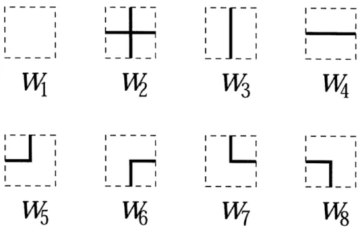
2-1 Possible configurations of dimers at each lattice site and their weights.

W1 = 4(X), w2 = O, w3 = W4 5 = 6 = 8 = . The only

allowed possibilities are either two dimers or zero dimers (a monomer) at a particular lattice site. This figure is taken from [2]. ... . 26 2-2 Configurations of loops in each of the four homotopy classes: ₀oo, £1o, ol,

and L11, where the time direction runs left to right. The + and - signs are the values of spins on the dual lattice. Figure taken from [1]. .... 27 2-3 Diagram of the relationship between coordinates on the original lattice

and dual lattice. A link exists on the original lattice between spins of opposite signs on the dual lattice. Figure taken and modified from [1]. 30

4-1 Chiral condensate of two free Majorana fermions (g2 _{= 0) as a function}

of the mass parameter computed for two square lattice sizes. ... 45 4-2 Mass susceptibility of two free Majorana fermions (g2 = 0) as a function

of the mass parameter computed for two square lattice sizes. ... 46 4-3 Chiral condensate of two interacting Majorana fermions (g2 = 0.1) as

a function of the mass parameter computed for two square lattice sizes. 47 4-4 Mass susceptibility of two interacting Majorana fermions (g2 _{= 0.1) as}

a function of the mass parameter computed for two square lattice sizes. 48 4-5 Chiral condensate as a function of the mass parameter for 2 Majorana

fermions on a 32 x 32 lattice with g2 _{= 0. e = (0, 0), e = (0, 1) and}

4-6 Mass susceptibility as a function of the mass parameter for 2 Majorana fermions on a 32 x 32 lattice with g2 _{= 0. e = (0, 0), E = (0, 1) and}

C = (1, 1) boundary conditions were used. ... ... 50

5-1 Exact and simulated chiral condensate of one free Majorana fermion as a function of the mass parameter on a rectangular lattice with T = 4 and L = 16. The boundary conditions of the simulation were sampled from the partition function Z00 + Z01 _{using the algorithm of § 5.1. . . 55} 5-2 Exact and simulated chiral condensate of one free Majorana fermion as

a function of the mass parameter on a rectangular lattice with T = 16 and L = 4. The boundary conditions of the simulation were sampled from the partition function Z00 + Z01 using the algorithm of § 5.1. . . 56 5-3 Chiral condensate of two interacting Majorana fermions (g2 = 0.1) as

a function of the mass parameter on an 8 x 8 lattice with fluctuating

boundary conditions... . . ... .... ... 57

5-4 Mass susceptibility of two interacting Majorana fermions (g2 = 0.1) as a function of the mass parameter on an 8 x 8 lattice with fluctuating

boundary conditions. . ... . ... 58

5-5 Mass susceptibility of two interacting Majorana fermions (g2 _{= 0.1) on}

an 8 x 8 lattice calculated directly from simulations and by taking the

numerical derivative of the condensate. . ... 59

5-6 Chiral condensate for L = 24 and L = 48 lattices with N = 8, g2 = 0.5, and m = -0.5775. T is the number of lattice points in the time

direction, and increasing 1/T corresponds to increasing temperature. 60 5-7 Left: x (computed on a 6 x 48 lattice) and XT=o (computed on a

32 x 32 lattice) for 8 flavors of fermions as a function of g2. Increasing

g2 corresponds to decreasing temperature. Right: X - XT=O for N = 8 as a function of g2. . . . . . . . . 62

5-8 Left: x (computed on a 6 x 48 lattice) and XT=O (computed on a 32 x 32 lattice) for 16 flavors of fermions as a function of g2. Increasing g2 corresponds to decreasing temperature. Right: X - XT=O for N = 16

List of Tables

2.1 Weights of the 16 possible configurations of spins around a plaquette, where we have used the fact that w(sl, s2, s3, S4) = W(-8 1, -S2, -S 3, -84). 31

3.1 Values of bond probabilities Pi and Ai for bond variables b(x). ... 36 3.2 The monomer density and integrated autocorrelation time computed

for three square lattice sizes and three boundary conditions using the cluster algorithm. The results are very close to the exact values. . . . 39

Chapter 1

Introduction

1.1

Cluster Algorithms for Efficient Monte Carlo

Simulations

When studying systems with large numbers of degrees of freedom, it is useful to treat these systems numerically on the computer, as it is often impossible to directly compute the partition function,

Z= Z e-H (1.1.1)

states

where 0 is the inverse temperature and H is the energy of the system. Instead, one can use Monte Carlo methods to randomly generate configurations of the sys-tem which have a high Boltzmann weight. In this case the partition function can be approximated as a suitably weighted sum over these randomly generated most probable states. Since expectation values of thermodynamic quantities are integrals over all possible states weighted by the Boltzmann distribution, we can also use these methods to calculate values of physical observables.

As an example, consider the Ising model in two dimensions. The Ising model is a collection of particles which lie on discrete lattice sites and which have a single property called spin that can take on values +1 or -1. The energy of the system is

derived from each particle's interaction with its nearest neighbors. The Hamiltonian for the Ising model is

H = -J sisj (1.1.2)

(ij)

where J > 0 is a constant, (ij) denotes nearest neighbor lattice sites, si is the value of the spin at lattice site i, and si E {+1}. From this, we can see that adjacent particles with the same spin contribute negatively to the energy of the system and those with opposite spin contribute positively.

The order parameter for the Ising model is the magnetization

M = (1.1.3)

or the absolute value of the average spin per lattice site, where N is the total number of particles. At T = 0, the lowest energy state is the state where all spins take on the same value, and M = 1. Because there are two possible lowest energy states, one with all spins taking on the value +1 and one with all spins taking on the value -1, the global spin flip symmetry (si -- -si) of the Hamiltonian is spontaneously broken in either of the two ground states. At very high temperature however, the equilibrium state is a disordered state with M = 0. At a critical temperature Tc, the system transitions from a state of spontaneously broken spin flip symmetry (characterized by a nonzero magnetization) to a state where the symmetry is restored (and M = 0). In order to study the properties of this phase transition using Monte Carlo techniques, we would like to have a method to compute the average magnetization of the system

as a function of temperature.

For an Ising model with N particles, there are 2N possible states, and thus it is

not practical to directly compute the average magnetization for this system. Instead, we would like to do so using only the most probable configurations, or those config-urations where the Helmholtz free energy (F = - In Z) is minimized. The simplest algorithms to randomly generate most probable configurations are local updating al-gorithms. One example of this type of algorithm is the Metropolis algorithm. During

one iteration of the algorithm, the program visits each lattice site and calculates whether the energy is made smaller if the spin at that lattice point is flipped. If

AH < 0, the spin is flipped with probability 1, and if not, the spin is flipped with

probability proportional to e-OAH where 3 is the inverse temperature. The system

evolves through computer time toward an equilibrium configuration. The drawback of the Metropolis algorithm and similar algorithms is they have a high autocorrelation times. That is, the number of iterations of the algorithm over which configurations are correlated is significant.

Cluster algorithms provide dramatic improvements on these local updating algo-rithms. Instead of flipping one spin at a time, cluster algorithms flip whole groups of lattice sites at once. Among the earliest cluster algorithms that were developed are those of Swendsen and Wang for the two dimensional Potts model [3] and Wolff for

O(n) models in two dimensions [4]. A sketch of a cluster algorithm of this type for

the case of the Ising model is as follows.

1. Choose a random spin on the lattice to be the first spin in a cluster.

2. Visit each of its nearest neightbors, and if the value of an adjacent spin is the same, then include it in the cluster with probability p = 1- e- 23. If the adjacent

point has opposite spin, do not include it in the cluster.

3. Visit the nearest neighbors of each of the newly added spins and continue grow-ing the cluster in this way until no more spins are added.

4. Flip the value of all of the spins in the cluster.

These steps will generate one new lattice configuration. Because many spins are updated at once, algorithms of this type greatly decrease relaxation times and auto-correlations.

When simulating phase transitions, we run into difficulty because of long correla-tion times at and around the critical point. Cluster algorithms have the advantage of greatly reducing the effect of critical slowing down. This allows simulations at increased lattice sizes, which leads to the reduction of finite-size effects. In this paper

we develop and implement a cluster algorithm to study the properties of Gross-Neveu model fermions.

1.2

The Gross-Neveu Model

The Gross-Neveu model is a theory of relativistic fermions in 1 + 1 dimensions (one space and one time dimension) with a four-fermion interaction. This model is both renormalizable and asymptotically free, and because of its simplicity was created to study the properties of more complex asymptotically free theories, such as QCD. The original action described by Gross and Neveu [5] is

S = d2

x i ()+ 1 (()(X))2 (1.2.1)

where V is a massless fermion field with two spinor indices and N flavor indices. This action is invariant under the chiral transformation

0

Spontaneous symmetry breaking of this chiral symmetry results in a nonzero value of the fermion condensate (4'4') and causes the generation of a fermion mass, which was described in [5].

For the computational tools we develop in this paper, it will be most convenient to write the Gross-Neveu action in terms of Majorana fermions, as presented in [1]. A Majorana fermion, which is its own antiparticle, will be represented by a Grassman-valued field (i with two spin components. One Dirac fermion can be written as a combination of two species of Majorana fermions as

1

= I( 1 +iK2) (1.2.3)

1

=

v(1

a theory with 2N flavors of Majorana fermions.

We will use Wilson's method for representing fermions on a lattice, which corre-sponds to replacing the mass term

mfm(x)O(x) -+ mO(x)(x) - 20, (x)8,0/(x). (1.2.5)

The Wilson discretization of equation (1.2.1) where we set r = 1 (as in [1]) written in terms of Majorana fermions is given by

S = E Cc(,c , + m - -0)- ( Tc)2] (1.2.6)

where 0, "*, and 0 are the forward, backward, and symmetric discrete derivatives on the lattice which act as

(Ta* = (T(x + :) - (T(x) (1.2.7)

8,r = (( + A)

+ ((x - 4) - 2()

and C is an antisymmetric matrix such that Cy,C- 1 = -y, . The Wilson term

(proportional to 0*0) breaks the discrete chiral symmetry ( --* -5 of the massless theory. This symmetry is restored in the continuum limit at a critical nonzero value of the mass parameter m, which will cancel the chiral symmetry breaking effect of the Wilson term, restoring the massless form of the theory.

The partition function for one free Majorana fermion on a lattice with definite boundary conditions e is

Z[m] = D eCSfree = Pf [C( , + m - 0*)] (1.2.8)

where Sfree is the action from equation (1.2.1) with g = 0 and Pf denotes the pfaffian. The partition function for N flavors of free Majorana fermions is just (Z [m])N. If we consider the mass parameter as x-dependent, m = m(x), then we can write the full

partition function for the Gross-Neveu model with N flavors of fermions in terms of derivatives with respect to m(x) acting on the N-flavor free partition function [1] as

ZGN = De - s = exp

{-

There are four possibilities for the c of equation (1.2.8). On a two dimensional lattice with T lattice sites in the time direction and L lattice sites in the space direction,

thepossible choices of boundary condition are e = (ET, EL) with CT, EL E {0, 1}, where

0 indicates periodic boundary conditions and 1 indicates antiperiodic boundary con-ditions.

1.3

_{Fermion Phase Transitions in 1+1 Dimensions}

The properties of Gross-Neveu fermions at nonzero temperature have been studied in [6], [7], and [81. What has been found is that at zero temperature, spontaneous symmetry breaking of the chiral symmetry causes the generation of a nonzero fermion mass. If we rewrite equation (1.2.1) as

S=

- a2

1

where a is a scalar field, then at zero temperature, a acquires a nonzero vacuum expectation value, (a) = a* and the a/ term can be interpreted as a fermion mass term. The action of equation (1.3.1) leads to the same correlation functions of the fermion fields as equation (1.2.1).

In the limit of an infinite number of flavors of fermions, it is found that at some nonzero critical temperature, T., the chiral symmetry is restored and the mass van-ishes continuously but nonanalytically through a second order phase transition. How-ever, for any finite N, the chiral symmetry is restored at any nonzero T due to the condensation of kinks and antikinks along the space dimension [6]. At low T, the potential of equation (1.3.1) has two symmetric minima at

+a*(T).

antikinks are alternating segments of +a*(T) and -a*(T). Because of the alterna-tion of these segments, (a) = 0. This means that there is only spontaneous symmetry breaking at T = 0 for a finite number of flavors.

In Chapter 2 we will derive two representations of fermions on the lattice-first, a loop representation originally derived by Gattringer in [2], and then a representation of Ising spins developed from the loop representation by Wolff [1]. In Chapter 3 we discuss a cluster algorithm for simulating free fermions in 1 + 1 dimensions and present results for monomer densities for free fermions which are in agreement with exact values. We discuss the Gross-Neveu model in Chapter 4. We present a modified cluster algorithm in order to simulate interacting fermions and obtain results for the Gross-Neveu model using a cluster algorithm for the first time. We calculate fermion correlation functions at zero temperature in different boundary conditions. In Chapter 5 we study the Gross-Neveu model at nonzero temperature. We present an original algorithm for simulating fermions with fluctuating spin boundary conditions, which is necessary in order to simulate fermions at nonzero temperature. We describe results for Gross-Neveu fermions at nonzero temperature for the first time using a cluster algorithm, and demonstrate a fermion phase transition for large N. We discuss our conclusions in Chapter 6.

Chapter 2

Representing Fermions on a

Computer

It is not possible to directly sample the action of equation (1.2.6) because fermionic fields are Grassman-valued. This means that we cannot sample lattice configura-tions of Grassman numbers because we do not have an efficient way of implementing Grassman numbers on a computer. In order to simulate fermions using Monte Carlo methods, we must first come up with a way of representing field configurations on the computer. One way of doing this is through a loop representation first described by Gattringer in [2]. He describes an equivalence between the two-dimensional Wilson fermion determinant and a sum over configurations of dimers on a lattice which form closed loops. In § 2.1 of this chapter, we rederive Gattringer's loop representation of the Gross-Neveu model. In § 2.2 we show the equivalence of this loop representation to a system of Ising spins on a lattice. In § 2.3 we discuss the extension of this spin representation to include negative values of the Gross-Neveu mass parameter. The derivations presented in this chapter follow § 3 of [1].

2.1

Rederivation of the Fermion Loop

Represen-tation

Here we will rederive the loop representation of [2] in the context of Majorana fermions with definite boundary conditions. Initially, we will ignore the four-fermion interac-tion term in the Gross-Neveu model and only consider the acinterac-tion for a free Majorana fermion in 1+1 dimensions:

S = (x)( ()C((x) - (x)CP(4)((x +

4)

X X41

where O(x) = 2+m(x) and P(n) = -(1-n,y,) for lattice unit vectors n =

+±.

is a projection operator formed from a combination of the discrete lattice derivatives of equation (1.2.6) and has the property

~T_{(x)CP(A)((x + A) = (T(x + 4)CP(-4)((x). (2.1.2)}

In order to calculate observable quantities, we would like to evaluate the partition function

Z [] =/ De -s (2.1.3)

where E specifies a boundary condition for the ( particles. Plugging equation (2.1.1) into equation (2.1.3), we get

Z [q] = Dexp [ (x)( T(X)C((x) +

(

We can expand the Boltzmann factor to O( 2_{) to obtain}

Z [] = J 1DF (1 + i(x)2(x)) 1(1 + T(x)CP(A)(x + 4)) (2.1.5)

where we have used the phase convention: -ITC( = (1(2. Now we reorganize this equation by introducing variables k(x, p) which can take on values 0 or 1 and summing

over all possible configurations of k(x, p) to obtain

Z[0] =

J

D

f(+

{k(x,p)} x X,I

These variables can be interpreted as dimers which lie on the links between lattice sites. If k(x, p) = 1, there is a dimer on the link between site x and site x +

ft,

k(x, p) = 0, there is none.

At each lattice site, there are only two possible cases which will contribute a nonzero factor to the integral in equation (2.1.6). The first case is that there are no dimers on any of the four links adjacent to x (k(x, p) = 0 for p = (±1, 0) and

1L = (0, +1)). In this case the relevant integral is just

J

which contributes a factor of O(x) to the overall weight of the configuration. These types of sites, with no adjacent links, are called monomers. Because of the properties of Grassman variables, the only other possible case is that there are two adjacent links at a particular site. Thus, there are seven types of allowed dimer configurations at a particular site, which are shown in Figure 2-1 (the second configuration shown has weight w2 = 0). When we consider tiling a lattice with these types of dimer configurations, it is apparent that the only possible lattice configurations are closed loops of dimers which do not intersect or backtrack.

We want to calculate the Boltzmann weight of one of these dimer loops. Consider a loop which traverses lattice sites (x1, x2, ..., x1), each consecutive pair of which differs

by one lattice unit vector, i. The Boltzmann weight of this loop is given by

I =

J

(2.1.8) The result of this integral is

i I I--f--

-I I

-I

,

I 2 *

Figure 2-1: Possible configurations of dimers at each lattice site and their weights.

w1 = ¢(x), w2 = 0, wa = w4 = 1, w5 = 6 7 = = . The only allowed

possibilities are either two dimers or zero dimers (a monomer) at a particular lattice site. This figure is taken from [2].

which can be obtained by writing the projection operators in terms of their eigen-vectors as in [1]. The Boltzmann weight of the loop in terms of Nc, the number of corners it contains, and v = 0, ±1, the number of complete rotations it makes, is

I = (-1)+2 - _{2 (2.1.10)}

So if a loop doesn't make a full rotation (v = 0), but instead winds around the lattice then there is an extra minus sign in the weight.

Because loops can wind around the torus, we can define distinct homotopy classes of loops. Closed loops which, do not wind around the lattice can be continuously reduced to a point, and thus are in the trivial homotopy class. If two loops wind around the torus in the same direction, they are also reducible to a point, and this type of configuration is still in the trivial homotopy class. However, configurations with odd numbers of loops winding in the same direction belong to distinct homotopy classes. Because loops can wind either trivially or nontrivally around the torus in each

of the two directions (time and space), there are four distinct homotopy classes of loops: £oo, Coi, £10, and L11, where 0 indicates an even number of loops winding in one direction (the trivial class) and 1 indicates an odd number of loops winding in one direction. Examples of configurations of loops from each homotopy class are shown in Figure 2-2. The purpose of the + and - signs in the figure will be explained in the next section.

+ + + + + + + + + + + + + -

+

L

+--+---

+

- -1+

Figure 2-2: Configurations of loops in each of the four homotopy classes: £o0, £10, £o, and £11, where the time direction runs left to right. The + and - signs are the values of spins on the dual lattice. Figure taken from [1].

We can use equation (2.1.10) to define the Boltzmann weight p[k] of a particular configuration {k} of dimers as the product over the weights of each individual lattice

4-++4-+

+ + + +

+++ + --+-+ - 4-

-site.

p[k] = w(k, x) (2.1.11)

where w(k, x) is the weight of site x in the configuration {k} of dimers and

O(x) if x contains a monomer

1 if 2 dimers at x separated by 7r

w(k,x) - (2.1.12)

1/V if 2 dimers at x separated by r/2 0 otherwise.

So far we have not taken homotopy classes into consideration. We define four partition functions-one for each homotopy class-by summing over all possible configurations of dimers within each class:

ZJ[ = p[k] (2.1.13)

{k(x,tp)}El'j

where i,j E {0, 1} indicate whether there exists a nontrivial loop winding in each direction. From equation (2.1.10) we see that the weight of a loop is positive for all configurations in Loo.

The following connections between the dimer partition functions and the fermion partition functions hold, which are described in greater detail in [1]:

4Z4o[k] = +Z 0[0] + Z 0o[] + Z l [0] + Z 1

4Z10[] Z 00["] + Z o[¢] - Z1 [] + Z '1[]

(2.1.14) 4ZO1 [] = -ZEO[] - Z o[] + Zl [0] + Z 1 []

4Z [] = -Z °[ ] + Z°[¢] + Z1[ - Z 1[].

These relationships can be inverted to obtain partition functions for the fermions with definite boundary conditions in terms of the different classes of dimer partition func-tions. For example, the partition function for fermions with antiperiodic boundary

conditions in time and periodic boundary conditions in space is

Zj0

[o]

The negative sign in front of Zo1[] means we have to sum contributions of negative weights and effectively amounts to the subtraction of statistics.

2.2

Wolff's Spin Representation

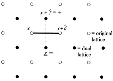
Here we sketch out the transformation of the dimer representation into a represen-tation of lattices of Ising spins. This is the crucial aspect for the development of a Swendsen and Wang style cluster algorithm. The general idea is to conceive the dimer loops as boundaries of domains of up and down Ising spins which lie on the dual lattice. We can make this mathematically concrete by putting a field s(x) of spins on the dual lattice and writing

k(x, p)= 1 if s(x)s(x + A) = -1 (2.2.1)

0 _{if s(x)s(x + A) = +1}

where {x} are the sites of the dual lattice, located at the centers of the plaquettes of the original lattice, s(_) is the value of the spin at x, and A is a unit vector on the dual lattice. A link on the original lattice (x,

i)

For each configuration of dimers, there are two possible configurations of spins on the dual lattice which obey equation (2.2.1). These two configurations differ simply by a global spin flip because, when populating the dual lattice with spins, there is a freedom in choosing the sign of the first spin. Examples of spins lying on the dual lattice can be seen in Figure 2-2.

o 0 0 0 X+

+

Figure 2-3: Diagram of the relationship between coordinates on the original lattice and dual lattice. A link exists on the original lattice between spins of opposite signs on the dual lattice. Figure taken and modified from [1].

all the plaquettes of the dual lattice, with a contribution w(sl, s2, S3, S4) from each

plaquette. If we label the spins around a plaquette as

(84

then we see that out of the 16 possible spin configurations, 2 are not allowed.

(

)

cannot exist because these correspond to intersecting loops on the original lattice. Therefore, though the spin fields s(x) are composed of Ising-type spins, the set of

allowed configurations is not equivalent to that of the Ising model.

We can define the weight of a plaquette on the spin lattice in terms of the relative signs of adjacent spins around the plaquette and unknown coefficients p, q, and r as

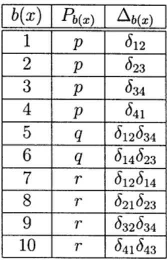
w(s, S2, S3, 84) = P[1262363441 L[23461423 +[114212363234+4143

where 6bi = (1 + sis) are bonds. Since the plaquettes on the dual lattice corre-spond to the lattice points on the original lattice of dimers, we need the weights of the plaquettes on the spin lattice to match the weights of the lattice sites in the dimer representation. By evaluating the delta functions for the different possible configurations of spins around a plaquette (as shown in Table 2.1), we find that

O(x) = 4p + 2q + 4r = 2p+r

1 = 2p + q.

(2.2.3)

Solving for p, q, and r, we obtain the dependence of these coefficients on the mass parameter: 1 r (2.2.4) P- 2V 2 q=1- +r. S1 82 83 S4 W(S1, 82,S3S 84) +(-) +(-) +(-) +(-) 4p + 2q+4r = (x) +(-) (-) -(+) 2p + r =1

+(-)-(+) +(-) +(-)

2p

+ r =

Table 2.1: Weights of the 16 possible configurations of spins around a plaquette, where we have used the fact that w(sl, s2, 83, S4) = W(-Sl, -82, -S3, -84).

We can now define four spin partition functions in definite boundary conditions as

Z= E H w(si, 2, 83, S4) (2.2.5)

{s() } plaq

where E is the boundary condition for spins on the dual lattice. In order to relate these spin partition functions to the dimer partition functions, Z(, we must realize

that a nontrivial loop configuration in the k-representation in one direction forces antiperiodic spin boundary conditions in the s-representation in the corresponding orthogonal direction. This means that the following relationships between partition functions hold

zoo _{_} ZOO s Z0 = Z Z Z1o Z = Z11 (2.2.6)

k' 2 s k 2 S ₂ s

where the 1 enters due to global spin flip symmetry. Note that for boundary conditions

E = (0, 1) and E = _{(1, 0), the antiperiodic direction is opposite in Zk and Z.}

2.3

Negative Mass

The three coefficients of equation (2.2.4) are positive for masses such that 0 < m < 2V/2. This is sufficient for the free theory since, in this case, m, = 0. However, for the theory of interacting fermions, it is necessary to allow for negative mass since

m < 0 due to additive renormalization. The current bond probabilities p, q, r given

in equation (2.2.4) restrict the algorithm we will use to m > 0 since otherwise r < 0 for negative m. In the negative mass case, we will need to use a new decomposition of the plaquette interaction by replacing the r term with

S[614 + 21623 + 632634 + 641643 + 612614 + 621623 + 632634 + 6416431

(2.3.1)

where 6_{iy - 1}

-bij are antibonds, and keeping the other two terms the same, but

making the substitutions p -+ jP and q -+ q. Setting the new weight and the old weight equal, we get the relations

r = -r

+

i- = p (2.3.2)

and plugging in the results of equation (2.2.4), we get the solution

- (- 2) = -m4

1 _(2.3.3)

2,2 2

We will need to use these alternate values when doing simulations with negative bare masses. The decomposition of equation (2.3.1) includes antibonds, which connect spins of opposite signs. This means that when using the cluster algorithm of the next chapter, if m < 0, clusters formed from these antibonds can include spins of both signs.

Chapter 3

A Cluster Algorithm for

Simulating Free Fermions

We have seen that free fermions in 1 + 1 dimensions can be represented as a system of Ising spins on a two dimensional latice. In order to calculate physical observables, we need a method to efficiently generate random lattice configurations. Since these fermions can be represented as Ising spins, we expect that it is possible to develop a method similar to the cluster algorithms for the Ising model of [3] and [4]. Cluster algorithms are much more efficient than local update algorithms. Here we develop a cluster algorithm for simulating free fermions in the spin representation. This algo-rithm constructs clusters of spins in order to generate independent spin configurations by using two Monte Carlo sampling techniques. In § 3.1, we describe the algorithm for simulating N flavors of free fermions on a lattice with definite spin boundary condi-tions. In § 3.2 we discuss the calculation of exact monomer densities for free fermions, and in § 3.3 we compare these exact calculations with free fermion simulations using the cluster algorithm of § 3.1.

3.1

Description of the Algorithm

We would like to sample configurations of spins from the partition function Z', for a fixed value of e. We will update spin configurations by constructing clusters of spins

and flipping the value of the spins in these clusters with some probability. As a first step, we will rewrite the weight of a single plaquette as

10

W(s 1,82 S2 S 3 4) E Ai(1,82, i S3 S4) (3.1.1)

i=1

where Pi E {p, q, r} and the A are the 10 delta function terms in equation (2.2.2). These Ai can be conceived as configuratons of bonds which lie on the links of the lattice of Ising spins. If 6ij = 1, there is a bond between si and sj, otherwise, there is no bond.

In order to construct clusters of spins, we will first sample the Ais. To do this, we will restructure the partition function as follows. Introduce bond variables b(x) which take on the values {1, ..., 10} and represent the 10 possible configurations of bonds around a single plaquette (see Table 3.1). Sum over all possible configurations of these bond variables on the original lattice in addition to all possible configurations spins on the dual lattice to get

ZS = :

I

{b(x),s(x)} plaq

With the partition function now written this way, we can sample both the bond variables and the spins. These three steps are required to generate one new spin

b(x) Pb(x) Ab() 1 p 612 2 p 623 3 p 634 4 p 641 5 q 612634 6 q 614623 7 r 612614 8 r 621623 9 r 632634 10 r 641643

configuration.

1. Choose a new configuration of bond variables, {b(x)}, at fixed spins by a local heatbath procedure. That is, sweep through the lattice and at each site x, choose a new b(x) e {1, ..., 10} with probability

p(b(x)) Pb(x) Ab(x)(s 1, 82, 83, 84) (313)

p(b()) 10(3.1.3)

SPiAi(s

i=1

Note that some values for b(x) may have zero probability because Ai(sl, 82, s2, 3,) =

0 for some i and some configurations of four spins. For example, for sl = s2 =

s3 = + and s4 = -, the only possible values for b(x) with nonzero probability

are b(x) = 1, 2, or 8 because A1, A2, and As are the only nonzero delta function terms.

2. Construct clusters of spins based on this new bond configuration. The set of bond variables {b(x)} maps out a configuration of bonds lying on links between spins. This bond configuration completely specifies the set of clusters. Two spins which are joined by a bond belong to the same cluster.

3. For each cluster, either flip all of the spins in the cluster or flip none of them. Choose each option with probability 1/2. This results in the selection of one of the possible equally weighted configurations of spins.

Performing these steps constitutes one iteration of the algorithm, after which we have sampled one new configuration of spins.

Simulating multiple flavors of fermions is trivial in the case of the free theory. Each flavor is represented by an Ising lattice of spins, meaning that for N flavors, there are

N spin values at each lattice point. Each of the N lattices is updated independently

according to the steps described above, and the update procedure for one lattice is not affected by the values of the spins in the other N - 1 lattices. This will no longer be true in the interacting theroy, and we will return to this discussion in Chapter

4. After each lattice has been updated, we have sampled one new configuration of

(Z[])N.

If we want to sample configurations of the spin partition function with boundary conditions other than E = (0, 0), we have to modify the algorithm such that spins which lie on an edge with antiperiodic boundary conditions see each other as the opposite sign. This only affects the weights of plaquettes along an antiperiodic edge, which should be adjusted for when computing bond probabilities.

3.2

_{Exact Monomer Densities for Free Fermions}

To test the effectiveness of our algorithm, we would like to compute an observable which can be calculated exactly. One such observable we can calculate is the average monomer density (K). K(x) = 1 if there is a monomer at x and 0 otherwise. In the spin representation, this is just

K(x) = 6151+S2+S3+841,4 (3.2.1)

which evaluates to 1 only if the four spins around x are the same. (K) can be computed exactly for free fermions in any combination of boundary conditions using the methods described in [1]. In the free theory (K) is directly proportional to the more interesting observable, the fermion condensate (V/4), or (ITC() in terms of Majorana fermions, as

(K) = -- ( TC() (3.2.2)

2

where = 2

+

because they are easy to compute exactly and because, as we move to the interacting theory, we will want to compute ( TC(). In the next section, we discuss calculations

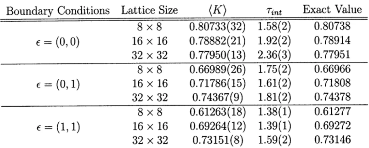
Boundary Conditions Lattice Size (K) Tint Exact Value 8 x 8 0.80733(32) 1.58(2) 0.80738 E = (0, 0) 16 x 16 0.78882(21) 1.92(2) 0.78914 32 x 32 0.77950(13) 2.36(3) 0.77951 8 x 8 0.66989(26) 1.75(2) 0.66966 E = (0, 1) 16 x 16 0.71786(15) 1.61(2) 0.71808 32 x 32 0.74367(9) 1.81(2) 0.74378 8 x 8 0.61263(18) 1.38(1) 0.61277 E = (1, 1) 16 x 16 0.69264(12) 1.39(1) 0.69272 32 x 32 0.73151(8) 1.59(2) 0.73146

Table 3.2: The monomer density and integrated autocorrelation time computed for three square lattice sizes and three boundary conditions using the cluster algorithm. The results are very close to the exact values.

3.3

Simulations of Free Fermions

(K) was computed using the cluster algorithm for three different lattice sizes and

in three different boundary conditions (E = (1,0) is equivalent to e = (0, 1) on a square lattice). The results of these simulations are shown in Table 3.2. The exact values are within errors of the results. Each run had 6 x 105 iterations, with a small fraction discarded to allow for equilibration. The integrated autocorrelation time Tint

measures the average number of iterations over which configurations are correlated and is given by N-1 Tint = 2 (t) (3.3.1) int-- --- E (0) t=1 where

F(t) = (aiai+t) - (ai) (ai+t) (3.3.2)

is the connected correlation of measurements ai that are t computer time steps apart, and F(0) is just the variance of the measurements. With this definition of Tint, the error a on the measurement is given by

2 2Tint (0). (3.3.3)

N

Values for (K), errors, and Tint were computed using the methods described in [9]. Both (K) and Tint are consistent with the results obtained by Wolff in [1]. The run

time scaled approximately as the order of the size of the lattice. Everything was computed on the order of minutes using a laptop.

In general, the autocorrelation time slightly increases with increasing lattice size. This algorithm is much more efficient than local algorithms, which have autocorrela-tions which scale with the lattice volume [1]. In addition, errors on the value of (K) decrease with increasing lattice size roughly as 1/TL, adjusted by the slightly increas-ing autocorrelation time. Tint is lower for simulations with increasincreas-ingly antiperiodic boundary conditions, as found in [1].

Chapter 4

Simulations of Interacting

Fermions

Now that it is possible to simulate free fermions on a two dimensional lattice using a cluster algorithm with efficiency much greater than that of known local updating algorithms, it would be much more interesting to apply this technique to the interact-ing theory, where correlation functions cannot be calculated exactly. In this chapter, we discuss the application of the cluster algorithm of Chapter 3 to the Gross-Neveu model. In § 4.1, we describe how to modify the algorithm to simulate N flavors of interacting fermions. § 4.2 discusses how to calculate fermion correlation functions using this algorithm. We present the first results of simulations of the Gross-Neveu model using a cluster algorithm in § 4.3 (for doubly periodic spin boundary condi-tions) and in § 4.4 (for singly and doubly antiperiodic boundary condicondi-tions).

4.1

Modification of the Cluster Algorithm

The algorithm described in § 3.1 must be modified in order to simulate N flavors of interacting fermions. To model N flavors of interacting fermions, we will use N Ising lattices (one for each fermion). This means that at each site there are N spins (one from each lattice.) The total weight of a particular configuration is a product over the weights of the plaquettes of each of the N lattices. The weights of plaquettes that

do not contain monomers are numerical constants and so are unchanged. However, the monomer weights are modified due to the interactions between fermions. w(x) = O(x) = _{2 + m(x) is replaced by an effective monomer weight O,(x) which depends on}

the total number of monomers at site x and the value of the coupling, g. The inclusion of these effective monomer weights is the only difference between the algorithm for the free theory and the algorithm for the Gross-Neveu model [1].

We can calculate these effective monomer weights using equation (1.2.9). If there are n monomers at site x, then the weight of site x comes from the interactions of all the monomers at x and is given by

c(n, m, g) = exp g₂ (2 +m)= 2J!(n 2j): 2(2 + m)n-2. (4.1.1) j=0

This means that we can replace O(x) with the effective monomer weight S= c((x) + 1, m, g)

() =(4.1.2)

where i(x) = number of monomers at site x in the N - 1 lattices not currently being updated. The first few effective monomer weight values are

o0(x) = 2 + m; l1(x) = 2+m + 2 2(x) = 2 + + 2g m m ) (4.1.3)

In one iteration of the algorithm, each spin lattice is updated independently. The effective mass only enters the update routine in the step where the bond variables are updated through the coefficients p, q, and r, which depend on the value of ¢.

4.2

Calculation of Correlation Functions

We would like to use our algorithm to generate most probable configurations of the Gross-Neveu partition function in order to calculate fermion correlation functions. We can test the correctness of our algorithm by computing these observables and comparing them to exact results at g = 0, and to results calculated by other methods

for g =f 0. Here we will derive equations for correlation functions in the spin repre-sentation. The observables we will discuss are the chiral condensate and the mass susceptibility, which can be written as derivatives of the partition function.

Define X, the chiral condensate, as

1 T In ZS

=(1 = lnZ) (4.2.1)

V 1m

where V = TL is the total number of lattice sites. The spin partition function from

equation (2.2.5) can be written as

Z = ds w(x) (4.2.2)

x

where f ds indicates a summation over all possible spin configurations and w(x) is the weight of the plaquette at x, taking into account the effective monomer weights from equation (4.1.2). Plugging equation (4.2.2) into equation (4.2.1), we get

1 1 aZ 1 1 w(x)

--,ds (Uw(x')

)(4.2.3)

V Z Om V Z Xm *

We can rearrange this by multiplying and dividing the integrand by w(x) to give

x=

Jds

Z(x)

V

Z

w

(x) am

The equation is now in the form X - -.

f

x

operator

1 w(x) (4.2.5)

Z.w (X)

am

for each spin configuration and average over these independently generated measure-ments of 0 to compute a value for X.

The mass susceptibility C_x is a measure of how the chiral condensate changes with an infinitesimal change in the mass parameter and can be written as the second

derivative of the partition function

ax

CX m V Om2 (4.2.6)

Following the same steps we used to compute the equation for X in the spin repre-sentation, we get

V

=m

V

_{(z) am}

1

1

1

w()

V

Z

ds

Z

W()

om2

w(x)2

Therefore, in order to compute Cx we have to sample the operator

w(x)

E ( 1 a2w(x) 1

+ w(x) iM2 W(x) 2

in each spin configuration and also use our calculated result for x. The derivatives of w(x) which appear in equations (4.2.5) and (4.2.8) are only nonzero if there is a monomer at x and can be computed by taking derivatives of equation (4.1.2). Calculations of X and Cx for the Gross-Neveu model are discussed in the next two

sections.

4.3

Results for the Gross-Neveu Model

The results presented in this section were all computed with c = (0, 0) spin boundary conditions with all spins pointing in the same direction as an initial condition. We begin with further results for the free case. The chiral condensate was calculated as a function of the mass parameter m using the cluster algorithm of § 4.1 and the prescription of § 4.2 for two free Majorana fermions for 8 x 8 and 16 x 16 square

Cx w())2) (4.2.7)

Sam

()

-5--)

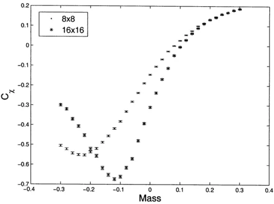
-0.6 * 16x16 S8x8 * -0.65 --0.7 -= -0.75 -= = * -0.85 -0.4 -0.3 -0.2 -0.1 0 0.1 0.2 0.3 0.4 Mass

Figure 4-1: Chiral condensate of two free Majorana fermions (g2 = 0) as a function of the mass parameter computed for two square lattice sizes.

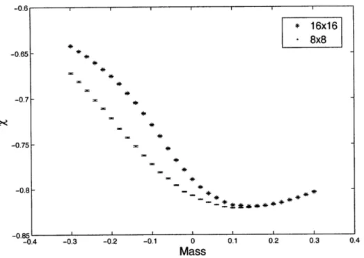
lattices and is shown in Figure 4-1. Similarly, the mass susceptibility was computed as a function of m for two free Majorana fermions and is shown in Figure 4-2. We used O(104) measurements of observables per data point, and could produce one curve in on the order of an hour using a laptop. The statistical errors for all of the measurements in this section were computed from integrated autocorrelation times using the methods of [9]. We see a peak in the magnitude of the susceptibility that moves to the right as the lattice size increases. This peak diverges logarithmically with L2 at m = 0, as calculated in [10] and [11] for lattice sizes up to 5122 and 7002. Similar plots were produced of X and Cx for one Dirac fermion using a loop

algorithm in [11]. The results we obtain for two Majorana fermions are quantitatively equivalent to the results obtained for one Dirac fermion, as expected. Therefore, we reconfirm that the cluster algorithm is working properly for the the free theory, and we conclude that our methods for computing X and Cx in the spin representation

0.2 0.1 * 16x16 b

S8x8

Figure 4-2: Mass susceptibility of two free Majorana fermions (g2 _{= 0) as a function}

of the mass parameter computed for two square lattice sizes.

laptop, and it is well within our capability to extend these calculations to larger lattice sizes, we do not feel the need to do so, as we expect to obtain results which are quantitatively equivalent to those presented in [11]. For the two lattice sizes we did explore, we observe that for m >-- 0.2, the values of X and Cx no longer differ. The differences at m <- 0.2 are due to effects from the finite size of the lattice.

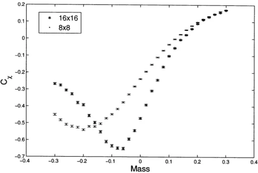
For the interacting theory, plots of the condensate and mass susceptibility for two Majorana fermions at coupling g2 = 0.1 are shown in Figure 4-3 and Figure 4-4 respectively. The shapes of the curves in the interacting case are qualitatively similar to those of the free theory, but the correlation functions take on different values due to the nonzero fermion coupling. These plots can once again be compared with plots obtained using a loop algorithm for one Dirac fermion in [11]. We find that the curves of X and Cx are equivalent to those in [11], and thus conclude that our

algorithm works properly for the theory of interacting Gross-Neveu fermions. The peaks in the susceptibility are shifted to the left from their location in the free theory

0

Mass

Figure 4-3: Chiral condensate of two interacting Majorana fermions (g2 = 0.1) as a function of the mass parameter computed for two square lattice sizes.

obtained in [11], we expect that the critical mass is no longer at m = 0, but occurs at a negative value of the mass parameter. Again, we see the disappearance of finite size effects at high values of the mass parameter. Though we have not computed correlation functions for lattice sizes greater than 16 x 16, we expect that finite size effects will also disappear with large lattice sizes at low values of the mass parameter and only remain manifest at the critical mass, as in [11].

These are the first results for the Gross-Neveu model using a cluster algorithm. The enormous improvement in efficiency over local algorithms make this algorithm an excellent tool to numerically study interacting fermions in 1 + 1 dimensions. In the next chapter we will use this tool to investigate phase transitions of interacting fermions. But before we conclude this chapter, we will present results for the Gross-Neveu model in spin boundary conditions other than E = (0, 0).

* 8x8 * 16x16 ** *** =4 *k 4 * * "* "1-f *g -0.2 -0.1 0

Mass

Figure 4-4: Mass susceptibility of two interacting Majorana fermions (g2 _{= 0.1) as a} function of the mass parameter computed for two square lattice sizes.

4.4

Boundary Conditions

Here we present results for interacting fermions in fixed spin boundary condtions E = (0, 1) and c = _{(1, 1). Figure 4-5 shows X computed as a function of the mass}

parameter for a 32 x 32 lattice with g2 _{= 0 for these three boundary conditions.} Because E = (1, 0) boundary conditions are equivalent to e = (0, 1) on a square lattice, E = (1, 0) was omitted. We see finite size effects due to the different boundary conditions. At small values of m, there is no distinction in the value of the condensate for different boundary condtions, however, at large m a gap emerges. This agrees with the results obtained in [11]. As the boundary conditions become increasingly periodic, the magnitude of the condensate decreases for high values of m, as was found in [11]. This is due to the fact that for e = _{(0, 0), there are no nontrivial loops on the latice,}

and at high mas there are a greater number of monomers than in the boundary conditions c = (0, 1) and E = (1, 1). Figure 4-6 shows Cx as a function of m on a

0.1 I -0.1 -0.2 -0.3 -0.4 -0.5 -0.6 -0.7 -0. 4 -0.3 S!II I I I . w I I

-0.4 -0.3 -0.2 -0.1 0 0.1 0.2 0.3 0.4

Mass

Figure 4-5: Chiral condensate as a function of the mass parameter for 2 Majorana fermions on a 32 x 32 lattice with g2 _{= 0. E = (0, 0), E = (0, 1) and e = (1, 1) boundary} conditions were used.

32 x 32 lattice with g2 _{= 0 for the same three boundary conditions. We see that the}

cusp in the mass susceptibility is sharper for doubly periodic boundary conditions,

E = (0, 0), indicating a steeper transition in the condensate at m = 0, as observed in Figure 4-5. At high and low values of m, there is no difference in Cx between the

I I I I I I I • E=(O,o) + E=(0,1) E=(1,1) I I I I I I II II -0.3 -0.2 -0.1 0

Mass

Figure 4-6: Mass susceptibility as a function of the mass parameter fermions on a 32 x 32 lattice with g2 = 0. E = (0, 0), e = (0, 1) and E = conditions were used.

2 Majorana 1) boundary 0.2 F 0 -0.2 -0.4 -0.6 -0.8 I I I i 4 -11 -0. I Ii

Chapter 5

Gross-Neveu Fermions at Nonzero

Temperature

Now that we have developed an efficient cluster algorithm to accurately simulate Gross-Neveu model fermions, we can use this technique to further investigate the properties of interacting fermions in 1 + 1 dimensions. We would like to observe the second order phase transition from spontaneously broken chiral symmetry to restored chiral symmetry which occurs at a nonzero critical temperature. We can analyze fermions at nonzero temperature by using boundary conditions which are antiperiodic in the time direction (this leads to the correct Fermi-Dirac distribution of particles.) From equation (2.1.15), we know that in order to simulate the fermion partition function with e = (1, 0), we have to simulate all four possible spin partition functions. Yet, this equation contains a negative contribution from the Z' partition function, so when simulated, we would effectively be subtracting statistics from our calculation of observables, wasting computer time. If we reach the infinite spatial volume limit, however, the boundary conditions in the space direction should not matter. Therefore, to avoid simulating a negative partition function, and to make our algorithm slightly simpler, we will leave the boundary condition in the space direction variable and instead simulate

which can easily be derived from equation (2.1.14).

To simulate fermions at nonzero temperature, we need to sample spin configu-rations from two different classes of boundary conditions, e = (0, 0) and E = (0, 1), which are periodic in the time direction and either periodic or antiperiodic in the space direction. This reversal of boundary conditions comes from the correspondence of spin and loop partition functions described in equation (2.2.6). In § 5.1 we de-scribe an algorithm for simulating the partition function combination of equation (5.0.1) using fluctuating boundary conditons. We test the accuracy of this algorithm by comparing simulations of free fermions to exact results for the free theory in § 5.2 and checking its self-consistency in the interacting theory in § 5.3. The results of the first simulations of Gross-Neveu fermions at nonzero temperature using a cluster algorithm are presented in § 5.4.

5.1

_{Fluctuating Boundary Conditions}

Here we construct an algorithm for sampling spin configurations from the partition function Ztot = ZO1 + Z°o. Now each of the N spin lattices will have an associated boundary condition variable which is independent of the boundary conditions of the other lattices. At each iteration of the algorithm, first all of the spins are updated using the procedure described in §3.1. Then the program will attempt to update the boundary conditions of each lattice of spins. The idea of the algorithm is to look for some axis perpendicular to the space direction, which we will call a horizontal cut(assuming the time direction points horizontally and the space direction points vertically.) Then, with some probability, flip the spins above the cut while leaving the ones below fixed and, at the same time, change the spatial boundary conditions. We are only interested in changing the spatial boundary conditions, so our axis must be a nontrivial loop in the time direction. Though we could in principle search for any loop which begins and ends at the same plaquette point and winds around the lattice in the time direction to serve as our boundary for flipping spins, it is simpler and just as effective to only search for a horizontal line.