Algorithms for particle remeshing applied to smoothed particle hydrodynamics

ALGORITHMS FOR PARTICLE REMESHING

APPLIED TO SMOOTHED PARTICLE

HYDRODYNAMICS

by

Nikhil Galagali

B.Tech., Civil Engineering(2007)

Indian Institute of Technology Madras

MASSACHUSETTS INSTITUTE1

OF TECHNOLOGY

SEP 2 2 2009

LIBRARIES

Submitted to the School of Engineering

in partial fulfillment of the requirements for the degree of

Master of Science in Computation for Design and Optimization

at the

MASSACHUSETTS INSTITUTE OF TECHNOLOGY

September 2009

@ Massachusetts Institute of Technology 2009. All rights reserved.

ARCHIVES

Author ...

//

School of Engineering

Aug 7, 2009

Certified by...

John R.Williams

Professor of Civil and Environmental Engineering

-L -

I

I

Thesis Supervisor

Accepted by ...

Jaime Peraire

Professor of Aeronautics and Astronautics

Director, Program in Computation for Design and Optimization

ALGORITHMS FOR PARTICLE REMESHING APPLIED

TO SMOOTHED PARTICLE HYDRODYNAMICS

by

Nikhil Galagali

Submitted to the School of Engineering on Aug 7, 2009, in partial fulfillment of the

requirements for the degree of

Master of Science in Computation for Design and Optimization

Abstract

This thesis outlines adaptivity schemes for particle-based methods for the simulation of nearly incompressible fluid flows. As with the remeshing schemes used in mesh and grid-based methods, there is a need to use localized refinement in particle methods to reduce computational costs. Various forms of particle refinement have been proposed for particle-based methods such as Smoothed Particle Hydrodynamics (SPH). How-ever, none of the techniques that exist currently are able to retain the original degree of randomness among particles. Existing methods reinitialize particle positions on a regular grid. Using such a method for region localized refinement can lead to discon-tinuities at the interfaces between refined and unrefined particle domains. In turn, this can produce inaccurate results or solution divergence. This thesis outlines the development of new localized refinement algorithms that are capable of retaining the initial randomness of the particles, thus eliminating transition zone discontinuities. The algorithms were tested through SPH simulations of Couette Flow and Poiseuille

Flow with spatially varying particle spacing. The determined velocity profiles agree well with theoretical results. In addition, the algorithms were also tested on a flow past a cylinder problem, but with a complete domain remeshing. The original and the remeshed particle distributions showed similar velocity profiles. The algorithms can be extended to 3-D flows with few changes, and allow the simulation of multi-scale flows at reduced computational costs.

Thesis Supervisor: John R.Williams

Acknowledgments

I would like to thank my advisor Prof. John Williams for his guidance and continued support. It has been a great learning experience working with him. I would also like to thank David Holmes for the discussions we have had during the course of this project. Heartfelt thanks also go out to Schlumberger for providing the financial support during the course of this project.

My stay here in Cambridge wouldn't have been half as exciting as it has been, with-out the company of friends here. I am indeed grateful to all of them. Specifically, I would like to mention Amit, Ankur, Rupa, Vignesh, Vivek R, Vivek J, Vijay, Abishek, Shashi, Vikrant and Sumeet for all the fun we have had. A satisfied tummy is a pre-requisite for anyone to do good research. I had the good fortune of having been part of a cooking group during my first year at MIT. Thank you Jaykumar, KP, Vivek and Lavanya for having shared the cooking drills with me and allowing me the luxury of enjoying homemade Indian dinner everyday. I also want to express my sincere gratitude to Laura Koller, Prof. Jaime Peraire and Prof. Robert Freund. They have tried to give the very best that an academic program can provide in terms of giving the freedom to pursue our research interests and making us feel at home away from

home.

Finally, I want to express my deepest love and gratitude to my brother, Vishal and my parents. Without their doting support and guidance, I am sure, I wouldn't have accomplished what I have.

Contents

1 Introduction and Motivation

1.1 Numerical Analysis of Fluids . . . ... 1.2 Particle Methods ...

1.3 Problem Addressed ... 1.4 Literature Review ...

1.5 Thesis Outline . . . . . ...

2 Smoothed Particle Hydrodynamics

2.1 Basic ideas of SPH ...

2.2 SPH formulation of the Navier-Stokes Equations . . . . 2.3 Boundary Treatment . ...

3 Adaptivity in SPH

3.1 Error Analysis of SPH formulation 3.1.1 Notation...

3.1.2 SPH in one dimension . . . 3.1.3 Uniform particle spacing 3.2 Particle Remeshing Algorithms

3.2.1 Coarse to Fine Remeshing . 3.2.2 Fine to Coarse Remeshing 3.2.3 Interpolation Theory . . . .

3.3 Spatially varying mesh . . . ..

13 13 13 16 20 21 23 23 26 27 29 . . . . . . . . . 29 .. . . . 30 .. . . . . . . . 30 .. . . . . . . . . 31 .. . . . . . . . 34 .. . . . . . . . . . 35 .. . . . . . . . . . 35 .. . . . . . 38 .. . . . 40

4 Model Testing and Verification 43

4.1 Boundary Conditions ... ... . ... 43

4.2 Time Integration ... ... ... 44

4.3 Particle Interaction . ... ... ... . . . . .. . 44

4.4 Flow past a cylinder ... . 45

4.5 Couette Flow ... . 46

4.6 Poiseuille Flow ... . 48

5 Computational Efficiency of Remeshing 51

6 Conclusions 55

List of Figures

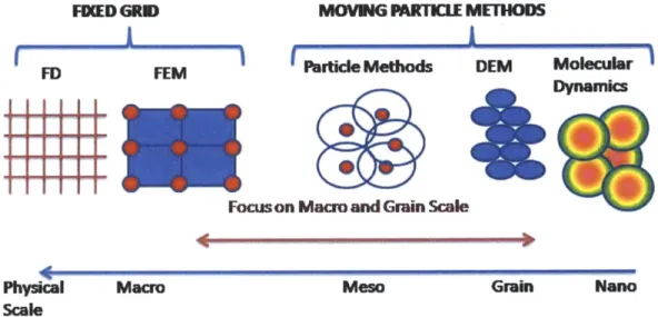
1-1 An overview of some of the major numerical schemes used for multi-scale simulations ... ... . 14 1-2 A typical 1-D flow with particle spacing transitioning from coarse to

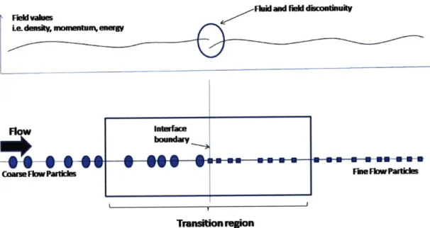
fine. Fluid and field discontinuity at the mesh interface is also shown. 17 1-3 Transition region in existing methods, which has virtual particles

cre-ated at regular locations; 1) Coarse-size particles are used to compute values for virtual fine-size particles at regular locations on a fine grid 2) Particle weights of neighbouring coarse-size particles are used to give values of coarse-size particles 3) Particle weights of neighbouring fine-size particles are used to give values of fine-fine-size particles 4) Fine-fine-size particles are used to compute values for virtual coarse-size particles at regular locations on a coarse grid ... . . . 18 1-4 Transition region in the new approach, which has virtual particles

cre-ated at positions that mimic real particles 1) Coarse-size particles are used to compute values for virtual fine-size particles at locations which mimic original distribution 2) Particle weights of neighbouring coarse-size particles are used to give values of coarse-coarse-size particles 3) Particle weights of neighbouring fine-size particles are used to give values of fine-size particles 4) Fine-size particles are used to compute values for virtual coarse-size particles at locations that mimics the original dis-tribution ... ... .. ... ... . 19

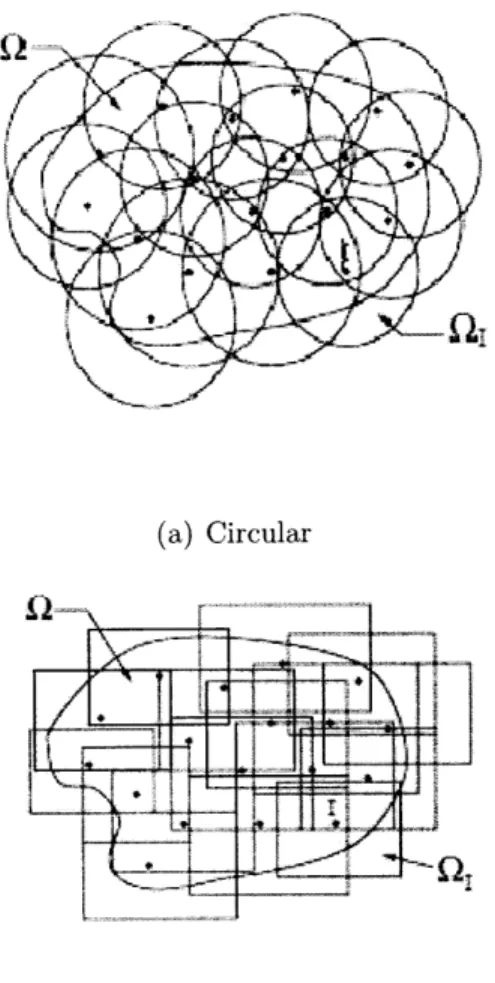
2-1 A computational model for a meshless method showing the boundary, nodes and support. (Source:Belytschko T., Krongauz Y., Organ D., Fleming M. and Krysl P. (1996), Meshless methods: An overview and recent developments, Comput. Methods Appl.Mech. Engg. ,139, 3-47) 24

2-2 Integral Representation and Particle Approximation . ... 25

3-1 Coarse to Fine Remeshing ... ... . . 36

3-2 Fine to Coarse Remeshing . ... .. . .. 37

3-3 Fine to Coarse Remeshing ... .... . 38

3-4 Interpolation function ... ... ... . 39

3-5 Transition of Flow from one mesh to another . ... 41

4-1 Flow past a cylinder with original particles(coarse) and the remeshed particles(fine) at different time steps . ... 46

4-2 Flow past a cylinder with original particles(fine) and the remeshed particles(coarse) at different time steps . ... 47

4-3 Couette Flow (Source:http://www.personal.psu.edu/wzl1113/Lesson Plan.htm) 47 4-4 Couette Flow ... ... 48

4-5 Poiseuille Flow (Source:http://www.personal.psu.edu/wzll113/Lesson Plan.htm ) ... ... ... 48

4-6 Poiseuille Flow . ... . . . . ... . 49

5-1 Domain used to study the temporal advantage of remeshing .... . 51

5-2 Time Comparison ... .. ... . 52

5-3 Snapshots . ... . . . . . . 53

A-1 The figure depicts the post-processor showing X-velocity at a certain instant of time ... . 62

A-2 The figure depicts the post-processor showing pressure at a certain instant of time ... . 63

List of Tables

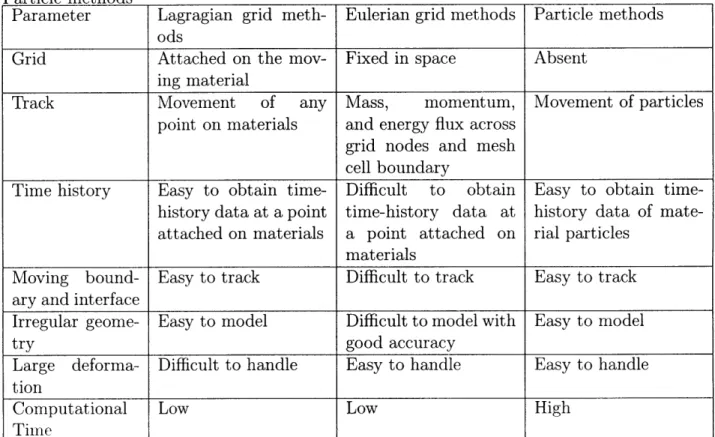
1.1 Comparisons of Lagrangian grid methods, Eulerian grid methods and Particle methods ...

Chapter 1

Introduction and Motivation

1.1

Numerical Analysis of Fluids

Computational Fluid Dynamics has been a widely used method to study fluid mo-tion for the last 50 years. Convenmo-tional methods like Finite Element Method(FEM) and Finite Difference Method (FDM) rely on a grid-based computational framework for spatial discretization. There are two kinds of grids that can be used for the dis-cretization. Firstly, an Eulerian framework(used in FDM), where the grid remains fixed in space and the material moves across the mesh. Secondly, a Lagrangian frame-work(used in FEM), where the grid moves along with the material. However, when simulating some special problems with large distortions, moving material interfaces, deformable boundaries and free surfaces, these methods can encounter difficulties. FEM cannot resolve the problems with large mesh element distortion. The Eulerian methods are inefficient in treating moving material interfaces. The Figure (1-1) gives an overview of some of the major numerical schemes used for multi-scale simulations.

1.2

Particle Methods

Meshless particle methods are a growing suite of methods used for solving partial differential equations. These methods have been shown to be very useful in solv-ing certain problems like multiphase flows, movsolv-ing material interfaces, deformable

Overview of Schemes for Numerical Modeling

FIED GRW MOVING PARTICE METHODS

SParticleMethods DEM Molecular

FD FEM

Dynamics

Focus on Macro and Grain Scale

Physical Macro Meso Grain Nano

Scale

Figure 1-1: An overview of some of the major numerical schemes used for multi-scale simulations

boundaries and free surface flows, where a conventional grid-based method, more of-ten than not, fails. Particle methods are a robust and versatile computational tool for the simulation of continuous and discrete physical systems ranging from Fluid Mechanics to Biology and Social Sciences. In advection dominated problems, particle methods can be considered as the method of choice due to their inherent robustness, stability and Lagrangian adaptivity.[1].

Smoothed Particle Hydrodynamics (SPH) is a meshfree, lagrangian, particle method originally developed for astrophysical applications[4, 5]. Since then, the method has been shown to be applicable to fluid mechaincs. Being among the very first parti-cle methods to be developed, the method has since evolved into a stable, consistent scheme for computational simulation of fluid motion. The paper by Monaghan[6] and the book by Liu and Liu [7] provide excellent reviews of the method's early growth and its recent developments. Like other particle methods, SPH relies on a set of disordered particles to obtain function approximations. In addition to being used as approximation points, these particles carry material properties and flow according the

Table 1.1: Comparisons of Lagrangian grid methods, Eulerian grid methods and Particle methods

Parameter Lagragian grid meth- Eulerian grid methods Particle methods

ods

Grid Attached on the mov- Fixed in space Absent ing material

Track Movement of any Mass, momentum, Movement of particles point on materials and energy flux across

grid nodes and mesh cell boundary

Time history Easy to obtain time- Difficult to obtain Easy to obtain time-history data at a point time-time-history data at time-history data of

mate-attached on materials a point attached on rial particles materials

Moving bound- Easy to track Difficult to track Easy to track ary and interface

Irregular geome- Easy to model Difficult to model with Easy to model

try good accuracy

Large deforma- Difficult to handle Easy to handle Easy to handle tion

Computational Low Low High

governing equations. SPH, like other particle methods, has advantages over the con-ventional grid-based methods when simulating deformable boundaries, multi-phase flows, free surface flows and irregular geometries.

1.3

Problem Addressed

In a typical numerical analysis by grid-based methods like Finite Element Method or Finite Difference Method, the size of discretization being used in a part of the domain is dependent on the accuracy desired in that region and the computational cost that the user is ready to expend for that. Larger mesh sizes are cheaper to solve compu-tationally, but yield inaccurate solutions. Consequently, using a uniformly fine mesh size in the entire domain would be a wasteful use of resource. To counter this diffi-culty, mesh adaptivity is used to vary mesh sizes in different regions. Interpolations are appropriately made to ensure compatibility and completeness of the solution.

Like the grid-based methods, there is a need to use adaptivity in particle-based methods to increase the efficiency and reduce the computational time(I-2). Attempts have been made in this direction by a number of authors in the past. Several studies of refinement and variable smoothing lengths in SPH exist in literature[21, 22, 23, 24, 25]. However, none of the techniques that exist currently are able to retain the original degree of randomness among particles. Particle methods enjoy the advantage of au-tomatic adaptivity. Flow strain may also cluster particles in some regions and spread them apart in others. This can lead to inaccurate simulations. To circumvent this problem, Cottet and Koumoutsakos[25] showed that the particles should be reini-tialized on a regular grid, and the properties of old particles interpolated on to new particles. However, this extremity of particle clustering or spreading doesnot happen regularly to warrant a repeated reinitialization on a regular grid. Reinitialization of particle positions on a regular grid can lead to discontinuities at the interfaces of the refined and the unrefined particle domains. This in turn leads to inaccuracies in fluid

density approximations or solution divergence.

FHuM and filid doninuuimly Le. deonk, wommom% emer

Fiwellk d d FineFk-lae

Transition region

Figure 1-2: A typical I-D flow with particle spacing transitioning from coarse to fine. Fluid and field discontinuity at the mesh interface is also shown.

consists of flow transitioning from a coarse particle distribution to a fine particle distribution. An overlap of the two particle regions is necessary to ensure accurate transfer of properties. In the overlap region, there exists corresponding virtual parti-cles used for making a two sided interpolation of field values. In the current schemes for particle adaptivity, these virtual particles are placed on regular grids. When the field approximations are made for the interface particles (as shown in circles) based on their respective neighbours, one typically obtains unequal results on either side of the interface. This regularly results in discontinuity in the field values. In addition, this type of reinitialization prevents a smooth transition of flow from one resolution to the other. This happens because after every time step the virtual particles are being reinitialized to their original positions, and hence virtual particles that would have moved closer to the interface than the grid point nearest to the interface, may not transform into real particles in the following time steps. This prevents a smooth continuity of flow when converting from one resolution to another.

Transition Region

t UlWarm s partice a Ilfhin pparticle

SVrbtualrenmied ars prtic Vrtualreenshd he particle

Figure 1-3: Transition region in existing methods, which has virtual particles created at regular locations; 1) Coarse-size particles are used to compute values for virtual fine-size particles at regular locations on a fine grid 2) Particle weights of neighbouring coarse-size particles are used to give values of coarse-size particles 3) Particle weights of neighbouring fine-size particles are used to give values of fine-size particles 4) Fine-size particles are used to compute values for virtual coarse-Fine-size particles at regular locations on a coarse grid

is one where they reinitialize all the particles, be it real or virtual on to a uniform grid at each time step. This approach is far more computationally expensive if the domain of study is large. The best approach to counter the above problem of interface discontinuity would be to remesh the particles on positions which resemble the original distribution (Figure 1-4). This thesis details schemes to do this. Algorithms are designed for transitioning from coarse to fine mesh and vice versa.

One of the prime examples of a place where such a remeshing strategy could be useful is in the simulation of geological porous media. A rock reservoir typically con-sists of many pores, which have to be modeled numerically to make an estimate of

Co+eFIPitid n 3 1u I'

aoprtcew

INrb2V Mnina rprtls ' SupportDomain Flow Partcls

i ile.denty o oantumn or enerw Smgerflid and fiedi

Transition raion

* Al coarse paicle a real ft paficl

* Virualrsrid coarse particl a VirtUalrWnhed fneu partick

Figure 1-4: Transition region in the new approach, which has virtual particles created at positions that mimic real particles 1) Coarse-size particles are used to compute values for virtual fine-size particles at locations which mimic original distribution 2) Particle weights of neighbouring size particles are used to give values of coarse-size particles 3) Particle weights of neighbouring fine-coarse-size particles are used to give values of fine-size particles 4) Fine-size particles are used to compute values for virtual coarse-size particles at locations that mimics the original distribution

the volume fractions of different components. Thereafter, the physics of the medium, consisting of multiple phases of fluids can be studied at a resolution based on the particle spacing in each region. A paper by Gerritsen and Durlofsky[2] provides an overview of some multi-scale modeling techniques to study oil reservoirs. Morris et al.[3] have detailed an SPH based numerical model to study flow through porous me-dia.

1.4

Literature Review

The resolution of particle simulations is dependent on the computational elements, namely the particles, and can be controlled to some degree by the particles' initial distribution. However, with time, the distribution of particles is dictated by the flow, and the local control of resolution is lost. In some applications, the distribution dic-tated by the flow leads to higher concentration of particles in some regions and a lower concentration in other regions. To ensure a good representation during par-ticle approximation, the smoothing lengths of parpar-ticles are varied from parpar-ticle to

particle. Shapiro et al.[14] extended this idea and allowed smoothing length to vary directionally. This approach however, is more suited to compressible flow simulations where the inter-particle separation varies markedly in different regions. In case of incompressible flows, the particle separation changes only by a small amount. But the particles move around to reach a state where the initial order is not retained. To improve the control of resolution in such circumstances, the particle distribution itself is changed. Kitsionas and Whitworth[21] have implemented a particle-splitting method for astrophysics. Liu et al.[10] presented an approach for inserting particles in an Eulerian form of the reproducing kernel particle method for CFD application. Later, Lastiwka et al.[22] developed a framework for adaptively inserting and remov-ing particles in smoothed particle hydrodynamics. In their algorithm, a new particle is placed near existing particle with a high velocity gradient. Its position is then iter-atively adjusted to improve the local inter-particle spacing. Feldman and Bonet[24] came up with a method for dynamic refinement. In their method, candidate parti-cles are split into daughter partiparti-cles in specific patterns governed by parameters like separation parameter. Following that, they solved a non-linear minimization problem to obtain the optimal mass distribution of the daughter particles so as to reduce the

errors introduced to the density field. Koumoutsakos et al.[25] have also presented accurate remeshing schemes for particle methods. However, all the above methods haven't been able to achieve the best density accuracy at the interface of the refined and the unrefined region.

1.5

Thesis Outline

In this thesis algorithms have been designed for remeshing particles while converting from a coarse mesh to a fine mesh and vice versa. Original particle randomness has been retained, but the spacing has been increased or decreased as per the requirement.

The thesis has been organized into six chapters. The current chapter gives a short comparison between grid-based and particle methods followed by the motiva-tion for the current research. The second chapter describes the Smoothed Particle Hydrodyanmics method, which is used as the particle method of choice for the idea demonstration. The third chapter begins with a short error analysis based on the available literature. Next, the algorithms designed for the remeshing are described. Finally, at the end of the third chapter, the interpolation stencil is detailed. The fourth chapter applies the algorithms to a few test cases. The algorithms have been tested through comparison of fluid velocities in a complete domain remeshing of flow around a cylinder. In addition, a spatially varying particle spacing has been used for tests on Couette Flow and Poiseuille flow. In the fifth chapter, a comparison is done between the computational times required for one cycle of simulation, with and without remeshing, for varying particle numbers. The final chapter summarizes the study and provides a direction for future research.

Chapter 2

Smoothed Particle Hydrodynamics

2.1

Basic ideas of SPH

A simulation that is based on SPH consists of material particles moving along a path prescribed by the governing Navier-Stokes equations and the given boundary and ini-tial conditions. The rationale of the method consists of using a kernel approximation for making an estimate of a function u(x) on a domain Q by:

uh(x) = w(x - y, h)u(y)dy (2.1)

Similarly, the kernel approximation of the derivative of the function is obtained by[7],

Vh(x) = - u(y)Vw(x - y, h)dy (2.2)

where uh(x) is the approximation, w(x - y, h) is the kernel or weight function,

and h is a measure of the size of the support(part of the domain that has an influence on the particle at x); in SPH works, it is often called a smoothing function or kernel function. According to Monaghan[12], the kernel is required to satisfy the following conditions:

(a) Circular

(b) Rectangular

Figure 2-1: A computational model for a meshless method showing the boundary, nodes and support. (Source:Belytschko T., Krongauz Y., Organ D., Fleming M. and Krysl P. (1996), Meshless methods: An overview and recent developments, Comput. Methods Appl.Mech. Engg. ,139, 3-47)

w(x - y, h) > 0 on a subdomain of Q, 2i

w(x - y, h) = 0 outside the subdomain Q21

Sw(x - y, h)d = 1 JQ

(2.3a)

(2.3b)

(2.3c)

w(s, h) is a monotonically decreasing function, where s = I|x - yjl. w(s, h) --+ 6(s) as h-+ 0, where 6(s) is the Dirac delta function.

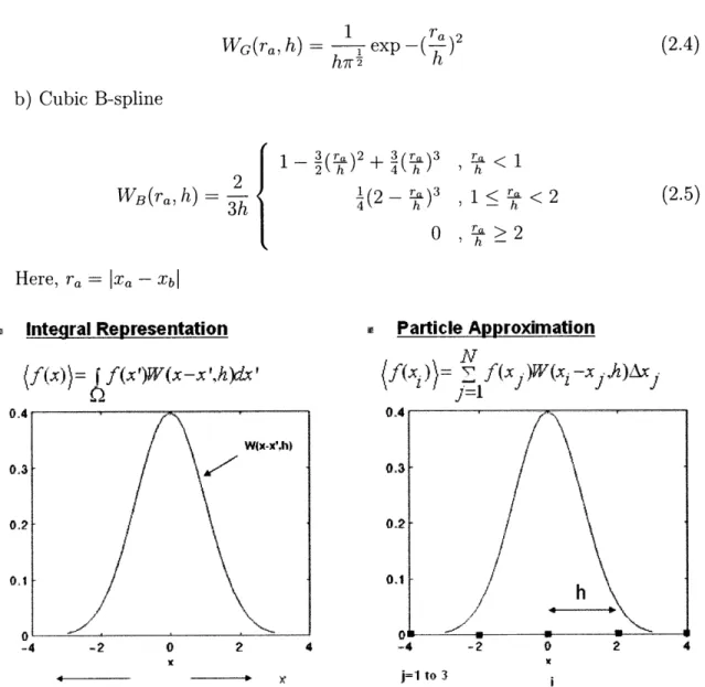
il-Some of the commonly used kernels are: a) Gaussian Kernel WG(Ta, h) = II h-r exp -(T 2 h b) Cubic B-spline WB(ra, h) = 1- (L)+_{2 h 4 h r h}< 1 1(2 - )3 , 1 < < ₂ h - h 0l _h-> 2 Here, ra = |Xa - Xbj Integral Representation (f(x))= f(x')W(x-x',h)dx' 12 9 Particle Approximation

f(xi)

Figure 2-2: Integral Representation and Particle Approximation

For a discrete distribution of particles, Equation (2.1) and Equation (2.2) give

h (Xa) = w (Xa - Xb, h)AVb W(a - b, h) _nz,b (2.

VUh(Xa) = - U (Xb)VW(Xa - Xb, h) b (2.4) (2.5) f (Xj)W(Xj -xjh)A', 6)

(2.7)

2.2

SPH formulation of the Navier-Stokes

Equa-tions

The governing equations for dynamic fluid flow can be written as a set of partial dif-ferential equations in Lagrangian description, commonly known as the Navier-Stokes equations. The Navier-Stokes equations consist of the following set of equations.

1) The continuity equation

Dp

Dt 2) The momentum equation

(2.8)

Dv" 1 &uO

Dt p ox, (2.9)

3) The energy equation

De a O

avo

Dt p 0X (2.10)

In the above equations a is the total stress tensor. It is made up of two parts , one part of isotropic pressure p and the other part of viscous stress T.

aP = -- p5P + T (2.11)

For Newtonian fluids,

ap = AEa3 (2.12) where 8v 8vo 2 cp =

+_

The SPH formulation for the Navier-Stokes equations with the particle approximation are [7]:

1) The continuity equation

Dpi _{m OWj}

(2.14)

Dt A P3 mvi OX,3

2) The momentum equation

DV _{Dv m.(} A _{+ Pj) Wij (} 118Wp ₊ 2) op a 8 if (2.15) Dt Pi Xi pi p ox with a r__ I0W __ WamjvOW a _ 2j mj = T- V~o

w-

3) The energy equation

Dei 1 Pi p OWij Pi E a (2.17)

Dt Dt 2 2 Em(\±-- pj 0 axi 2.2pi

2.3

Boundary Treatment

Treatment of boundary in SPH requires special considerations. The accuracy of the solution near the boundary is affected due to particle deficiency, which results from integral that is truncated by the boundary. For particles near or on the boundary, only particles inside the boundary contribute to the summation of the particle inter-action, and no contribution comes from particles outside the boundary because there are no fluid particles. To counter this difficulty, two types of virtual particles are used to treat the solid boundary conditions. The studies by Liu et al.[8, 9] recommend

using Type 1 virtual particles on the boundary and Type 2 virtual particles to fill in the boundary. The positions of Type 2 virtual particles are constructed in the fol-lowing way. For a certain real particle i, if it is located within distance khi from the boundary, a virtual particle is placed symmetrically on the outside of the boundary. These virtual particles have the same density and pressure as the corresponding real particles but opposite velocity. However, these Type 2 virtual particles are not suffi-cient to prevent the real particles from penetrating outside the boundary. Hence, the virtual particles of Type 1 are used. These Type 1 particles exert repulsive boundary forces on the real particles when the real particvles near the boundary.

The repulsive force is calculated using an approach that is similar to the one used for calculating the molecular force of Lennard-Jones form. If a particle of Type 1 is the neighbouring particle that is approaching the boundary, a force is applied pairwisely along the centerline of these two particles.

D[(-ro- )nl -( 2]( >)n2j

TO)1

PBij= i r ) r r - (2.18)

0 (ro) < 1

where the parameters ni and n2 are usually taken as 12 and 4 respectively. D is a problem dependent parameter, and should be chosen to be in the same scale as the square of the largest velocity. ro is usually selected approximately close to the initial particle spacing. It should be noted that position and physical variables do not evolve in the simulation process. The position of the Type 1 virtual particles remains fixed whereas the Type 2 particles are produced symmetrically according to the corresponding real particles in each evolution step.

Chapter 3

Adaptivity in SPH

3.1

Error Analysis of SPH formulation

Errors that occur in SPH formulations are a function of the smoothing length h and the ratio of the particle spacing to the smoothing length-. A study conducted by Quinlan, Basa and Lastiwka [15] shows that for uniformly spaced particles in one dimension with constant

f-

The SPH approximation to the gradient of a function u(x) at a particle a is given

by:

Vu(Xa) = - U(Xb)VW(Xb- ah) b (3.1)

b Pb

where W(x - xa, h) is the kernel function which tends to zero with increasing

distance between x and Xa. The summation is taken over all the particles b within

the compact support for the point Xa. The Gaussian kernel function defined by

Equation(2.4) and cubic B-spline defined by Equation(2.5) were some of the popu-lar early choices. Lately, higher-order spline kernels have also been used for SPH simulations.

Boundary smoothness of a kernel function is defined for the purposes of the fol-lowing analysis as the highest integer / such that the /3th derivative and all lower derivatives are zero at the edges of the compact support. That is

W(n)(-2h, h) = W(")(2h, h)= 0 for 0 < n < P (3.2a)

W(n)(-2h, h) = 0 or W(n)(2h, h) $ 0 for n = /3 + 1 (3.2b)

B-spline kernel has / = 2. Actually,/3 - oc for the Gaussian kernel, but since the kernel is used over a finite domain, the kernel and its derivatives do not decay to zero within the domain. Hence, /3 is not well defined for a kernel with infinite support.

3.1.1

Notation

The kernel and its derivatives in dimensionless form for the 1D case is given by:

X - Xa Xb- Xa Wa(s) = hW(x - xa h), s = - , Sb h(33) OnW(x - Xa, h) 1 d"W 1 h-(n) (3.4) Ox hn+1 8sn hn+1 2h f(x)dx h f(s)ds (3.5) J Xa-2h -2 3.1.2 SPH in one dimension

The error expressions that we obtain here are for 1D case simplicity. However, it can

be extended to higher dimensions similarly. SPH Error in the integral or smoothing stage of the approximation has been considered by Monaghan[6] and many others. In the integral in Equation (3.1), if u(x) is smooth, it can be expanded by Taylor series about Xa. With integration by parts, it results in

fXa±2h

2h (X) ox- ,, h) dx

u(,)

Xa-2haxO J,-2h

82U(X

a+2h

+ Xd2 ) xaa+2h (X - xa)W(X - Xa, h)dx

X a-2h 1 3U(xza) fXa+2h

+ x2h (X - Xa)2W(x - Xa, h)dx t3.6)

2

aZx

Expressed in a non-dimensional form of the kernel, the smoothing error is given by

- W'udx - u' = u( ds - 1) +hu"

sds+

With a normalized and even kernel, the first two terms on the right-hand side vanish. The error is then

- W'udx - u = a " S2Wds + O(h4) (3.8)

which is second-order in h. This is the contribution to the error due to the smoothing stage and is independent of particle distribution. Discretization error and the resultant overall error are considered next.

3.1.3 Uniform particle spacing

Because we are studying nearly incompressible flow, it is reasonable to assume that the spacing of the particles is uniform everywhere. The error obtained on introducing particle approximation to Equation (3.1) is Discretization error. Each particle b is located xb and associated with a volume (length in 1D) AXb. Here it is assumed

that the volumes span the compact support without gaps or overlaps. Since the particles are evenly spaced, Axb = Ax for all b. The approximate SPH integral can be described usefully by the second Euler-MacLaurin formula[16]. For a general function f(x), this is

n ,xn+Ax/2 B2kAx 2k ( 2k) __ (2k1 (

AX f -] f (x) + 2k! (1 (2-2n+1/2) - 1)) (3.9)

j= 1 Jx-Ax/2 k=l

where fj is defined as f(xi + jAx) and f(x) is smooth. B2k are the Bernoulli numbers, which increase non-monotonically with k, but not as rapidly as (2k)! in the denominator. If f(x) is defined as u(x)W'(x) for the present problem, the left-hand side of Equation (3.9) is identical to the SPH estimate of u'(Xa), the first term on the right-hand side represents its integral counterpart, and the remainder is an exact expression for the discretization error.

f,212

For typical kernels, some low-order derivatives are zero at the compact support boundary. This property of the kernel is described by the boundary smoothness

defined above. If the boundary smoothness of the kernel W is

/,

smoothness of the function u(x)W'(x) is 3 - 1, and the term fn2k-) - 1) in the

Euler-MacLaurin formula is zero for all 2k - 1 <

/

3

/3

UbWbAX -

JuW'dx

Ax0+2 B3+2 (1 - 2--)[(uW )' ( 1)+ - (uW') ( 3 + O(Axo+t$.10)

(0

+

2)!

u(x) in the error term is now expanded in a Taylor series about Xa, and the kernel is written in the non-dimensional form to make its dependence on smoothing length explicit. Derivatives of uW' are then expressed as follows:

h= + W(O + 2) + h sW 2) + ( + 1)W 1_)]

+

2h+1

0(_-.11)

This representation is now substituted into the term in square brackets in Equation(3.11)

and evaluated at x = za ± 2h. cancel to give [(uW') (,+ l ) - (uW')X(3-1 ₂h] ~" [4w+ 2

+ 2(139

If the kernel is even, even-order derivatives of u(x)

+

-+ 6(0-+1)/3 l=2 21

(3.12)

Substitution of this expression into Equation(3.11) leads to this final statement of discretization error

ZubU'Ax

h

( + 2)!

This can be combined with Equation(3.8) for smoothing error to obtain the fol-lowing expression for overall error:

-ZEUbWAX -U'a 2 +2 x, /\~ o L

a[4W=if2 + 2( + 1)W

It is clear that the total error is the sum of a second-order error in h(smoothing error) and an order (/3 + 2) error in Ax/h (due to discretization of the smoothing integral). The coefficient of (Ax/h)3₊2 _{in the discretisation error contains terms of the}

second order in h, as well as terms that are independent of h. Therefore, as Az/h is reduced, accuracy becomes limited by smoothing error of order h2. On the other hand,

as smoothing length h tends to zero , error does not vanish, but becomes dominated by a residual term which depends on Az/h. The kernel boundary smoothness, 3, determines the behaviour of this error term.

3.2

Particle Remeshing Algorithms

Depending upon the order of accuracy required in a certain domain of simulation, there is a need to be able to convert from one particle spacing to another. As de-scribed in the Introduction, a number of approaches have been devised by researchers. However, the challenge is to, atleast to a large extent, be able to retain the original randomness among the particles in different regions of the domain. The existing methods remesh the particles on a regular grid and then work out a way to assign the field values to these new particles. Retaining the original degree of randomness would be critical in getting higher accuracy at the interface of two different mesh densities. Besides, it will help in making an estimation of the phenomena at the boundary surfaces more reliable.

What we need is to be able to convert from a coarse to a fine mesh of particles and vice versa, while satisfying the conservation laws of mass, momentum and energy. In addition, the original particle distribution has to be retained with the particle spacing being scaled up or down equally in all the regions. This ensures that the local density fields of the bulk fluid are maintained to the original value. The remeshing process can be split into two parts.

a) Particle Position Determination b) Field Interpolation

Particle Position Determination is analogous to the grid generation that is done in grid-based methods. The idea is to come up with the locations of the new particles which satisfy the conditions in the last paragraph. Following the determination of the particle positions, the field variables like mass, momentum and energy have to be interpolated on to the new particles, ensuring that the conservation laws are satisfied. In the next two sections we describe the methodology for position determination of the new particles while converting from a coarse to a fine mesh and a fine to a coarse

mesh, respectively.

3.2.1

Coarse to Fine Remeshing

As the idea being discussed here is tailored for incompressible flow simulations, we shall adhere to the assumption that the spacing between a particle and its neighbours is nearly equal. Hence, the particle spacing is uniform throughout with variations of ±5 percent(as no liquid is an ideal incompressible fluid). Because all particles are equally(with slight variation) spaced from its neighbour, obtaining a distribution with a higher density and the same randomness is straightforward. For each particle, we need to find its respective neighbours and create a new particle at its mid-point(3-1). Neighbour here refers to particles that are at distances h ± 5%h from it. This way, we have ensured that particle density has increased uniformly, and the regions with slightly higher particle density continue to have a higher particle density. The new particles that are created are, like the original particles, are identical. Conse-quently, the mass of each of the new particles is equal. Since mass is conserved, the new particles are given a mass of total original mass divided by the number of new particles.

3.2.2

Fine to Coarse Remeshing

Remeshing from a fine to a coarse particle discretization is a more difficult proposition. The goal now is to get a particle distribution that gives a magnified representation of the original particle arrangement. However, the particle spacing cannot be simply

scaled by a constant factor because the size of the domain being remeshed is fixed.

Coarse

particlee

(a)

Coarse

*

0

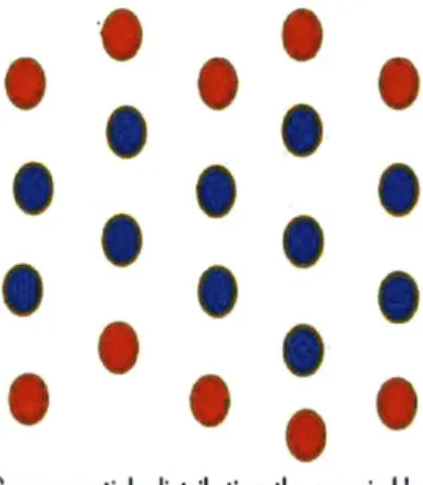
Coarse particle distribution, the ones in blue are fuid particles and the red ones are

boundary particles

(a) Coarse Mesh

*

0

0*0

(b) Fine Mesh (b) Fine Mesh

Figure 3-1: Coarse to Fine Remeshing

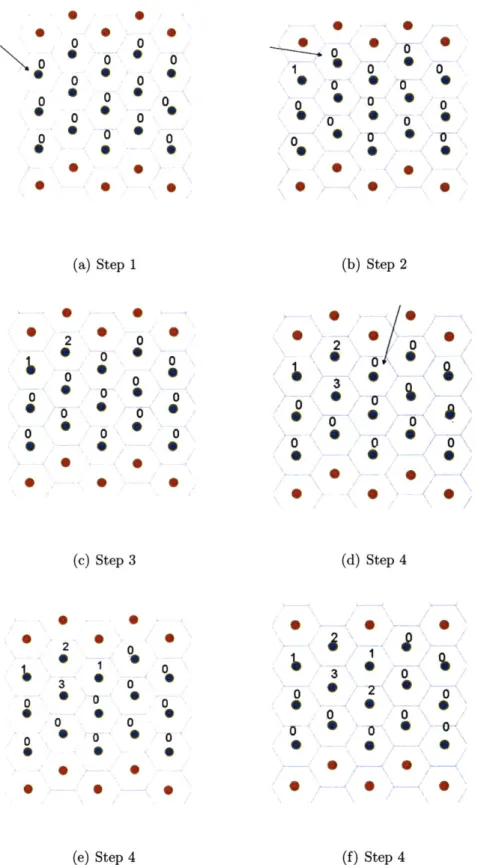
To come up the new particle arrangement, the following scheme has been devised: Step 1: Given a domain that is to be remeshed (3-2(a)), we give a tag to all the particles. For our purpose, we assign a number 0 to all of them.

Step 2: Take the first particle and search for its neighbours. Check the numbers currently on the neighbours and if all are 0 assign 1 to the first particle.

Step 3: Move over to the second particle. Search its neighbour and assign the lowest Natural number that doesn't exist among its neighbours. In this case it would be 2 as one of its neighbour already has 1.

Step 4: Continue this way for all the particles. We would reach a situation where the neighbours of a particle are 2,3... and 0. In this case , the current particle will get a number 1 assigned to it. Similarly, if the neighbours are 0,1,3..., then the particle is assigned a new tag of 2.

Step 5: Once all the particles have been numbered in this manner, one of the natural numbers is chosen and all the particles with tags other than this number are deleted from the domain.

* • o ₀ o₀ S 0 o0 0 0 _{0 0} 0 0 * • (a) Step 1 2 0 0 0 -0 *0 0 -0- 0 0 0 S0 0 * 0 • 0 0 () • • ) • - • (b) Step 2 2 0 0 0 0 0 * 0 • • • a) r, 0 0 o o 0 0 0 6 0 g (c) Step 3 (d) Step 4 * 2 0 2 3 0 0 0 * 0 o* 0 * • *) 0 --- 0 3 0 0 0 2 " 0 0 0 0 0 * * 0 * 0 0

(e) Step 4 (f) Step 4

S 2 2

0

3 3

2 2 2

•

.

. .

*

.

(a) Step 4 (b) Step 5

Figure 3-3: Fine to Coarse Remeshing

Figure (3-3(b)) shows the final result which is a coarse particle representation of the original fine distribution of particles.

3.2.3

Interpolation Theory

Once the particle positions have been determined, the field variables like momentum, energy are interpolated so as to satisfy the conservation laws. For this purpose, two types of interpolation formulas are used as discussed by Chaniotis, Poulikakos and Koumoutsakos [25].

Ordinary Interpolation

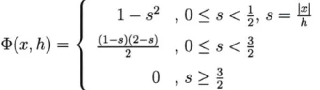
The interpolated quantity (zero order moment) as well as its first(impulse) and second moment(angular impulse) are being conserved by this second-order ordinary interpolation formula [17, 18].

1-_82 0 <1, s= IX - 2 h

D(x, h) = (2-) < (3.15)

0 ,s>3_2The

manner in which this interpolation formula is applied is shown as:

AQj(!2) = Qj(xj)4D(il - xj, h), (3.16) Support domain of particle i Old particle h - -- New particle

A

uii

i

h

i-yj

Figure 3-4: Interpolation function

which means that the jth old particle from location xj with property

Qj

particle which is in position i the interpolating quantity AQj. The interpolation in higher dimensions is obtained using tensorial products in each coordinate direction. This formula for two dimensions can be written as

AQ(i, >) = Qj(xj, yj) (i - xj, h) (i - yj, h) (3.17)

The interpolated quantity Qj must be an extensive property of the particle that is conserved.

O(x,h)= mju (3.18)

Ej

where mj is the mass of the particle, mju, and mjvj are the u and v momentum of the particle and Ej the total energy of the particle.

Smoothing Interpolation

The smoothing interpolation formulas attempt to minimize the error that the ordinary interpolation might produce, providing us with a moment conserving inter-polation, which is continuous everywhere inside the interpolation stencil

1-

2 2

h

M '(x, h) = (1-s)-s)s)2 1 < s < 2 (3.19)

0 ,s>2

The interpolation function and also its first and second derivative are continuous and reproduce second-order polynomials. This interpolation is used in the present SPH implementation in the main computational domain, away from solid boundaries.

Interpolation near solid boundaries

The remeshing procedure with ordinary or smoothing interpolating formulas can-not be used near solid boundaries. The interpolating stencil may extend to the inte-rior of the body, which introduces spurious computational elements. Hence, in regions near boundaries we use a biased ordinary interpolation [17], which is again second order and conserves the same quantities as the ordinary interpolation(conserves the first two moments and the quantity Qj)

1 - I ₂ + S2 for first cell from the wall, s = 1I_h

s(2 - s) for second cell from the wall,

S(x, h) =

(3.20)

for third cell from the wall, 2

0 otherwise

3.3

Spatially varying mesh

A spatially varying particle spacing is a necessity to make a practical use of the remeshing method. A profitable approach is one in which we only use a fine mesh in regions where we actually need high accuracy. Other regions, where we do not desire

SFlowdirection

Transition region

* Real coarse particle * Real fine particle Virtual coarse particle e Virtual fine particle

Figure 3-5: Transition of Flow from one mesh to another

a very high accuracy can be studied with a much coarser mesh. Hence, we need to use a spatially varying particle mesh. SPH, by its very interpolation nature requires a set of neighbours for remeshing to be accurately carried. For this we need to have a transition region, where we have both the coarse and the fine mesh simultaneously existing. At every time step, the original set of particles in the transition region are used for the creation of new particles. These new particles are termed virtual particles. The new virtual particles along with the old particles are moved according to the SPH governing equations. If the virtual particles cross the transition boundary in a time step, they turn into real particle. In the same way if a real particle crosses the boundary, it turns into a virtual particle. However, if the virtual particle does not cross the boundary in the time step, they are deleted and a new set of virtual particles are created with the remeshing method.

Chapter 4

Model Testing and Verification

For the purpose of verification of the above described idea, three sample problems have been tested. In the first problem, flow past a cylinder has been simulated with the remeshing algorithm being applied throughout the domain. This is a good measure of how the particle positioning and the interpolation scheme work when applied at every time step over the entire domain. A more practical implementation test of the method is when spatially varying mesh is used instead of a complete domain remeshing.

In the second and the third problems, Couette Flow and Poiseuille Flow are sim-ulated in SPH with spatially varying remeshing and compared with analytical results for the same.

4.1

Boundary Conditions

All the boundary particles are modeled by boundary particles that have similar phys-ical properties to those of the particles that represent the flow field. These particles interact with the flow particles in such a way that the necessary boundary condi-tions like the no-slip are satisfied. The no-slip condition is implemented in the form suggested by Morris, Fox and Zhu[20].

4.2

Time Integration

A predictor-corrector time integration scheme is being used for the SPH simulations. The time step is being taken so as to satisfy the Courant-Friedrichs-Levy (CFL) con-dition. The explicit time integration schemes are subject to the CFL condition for stability. The CFL condition states that the computational domain of dependence in a numerical simulation should include the physical domain of dependence, or the maximum speed of numerical propagation must exceed the maximum speed of physi-cal propagation.[19]. The CFL condition requires the time step to be proportional to the smallest spatial particle resolution, which in SPH applications is represented by the smallest smoothing length.

At = min(h) (4.1)

c

The time step to be employed in an SPH application is closely related to the physical nature of the process. Monaghan[6] gave two expressions when taking into

account the viscous dissipation and the external force.

h

At, = min( ) (4.2)

ci + 0.6(aci + /,maxz(oi))

hi+

Atf = min( )2 (4.3)

where f is the magnitude of force per unit mass.

4.3

Particle Interaction

In SPH simulations most of the computational time is taken up in the particle search-ing step. Because the smoothsearch-ing function has a compact domain, only a finite number of particles that are within the support domain contribute to the function approxima-tion. Hence, it becomes imperative that the particles in the support domain, refered to as nearest neighbouring particles in SPH literature, are quickly found. For this,

two kinds of searching algorithms are found to be most efficient. The Linked-list al-gorithm and the Tree-search alal-gorithm. Linked-list search alal-gorithm is best for cases when the smoothing length is constant in the entire domain. In the implementation of the linked-list search method, a temporary mesh is laid over the domain. The mesh spacing is usually taken as constant equal to kh. In some cases, the mesh spacing may also vary spatially. Each particle is then assigned to a cell and all the particles in a cell are chained together into a list. The advantage of laying this temporary mesh is that for each particle, the search for a neighbouring particle now has to be performed

only in its own cell or its neighbouring cell. The complexity of this algorithm is of order O(n). In contrast, an all-particle search is of order O(n2). In this thesis, we

are taking constant smoothing length, and hence the Linked-list search algorithm is used. The Tree-search algorithm is well suited in cases when the smoothing length varies spatially.

4.4

Flow past a cylinder

In this first test case, complete domain remeshing is implemented on a flow past a cylinder problem. This is a good test to view the behaviour of the method over a long duration of time with arbitrary particle locations in 2D. The remeshing algorithm for both the ways, coarse to fine and fine to coarse, have been tested and the velocity profiles over the entire domain compared through particle colour contouring. Periodic boundary conditions have been used in the X and Y directions to ensure continuous wrapping of flow.

In Figure(4-1) and Figure(4-2), the top flow corresponds to a full SPH simulation running in 2D whereas the particle flow beneath each of them are their remeshed counterparts. The particle distribution in the bottom half is determined by applying the remeshing algorithm at each step to the top distribution, and not by applying the SPH governing equations. The colour contouring is done based on the velocities of the particles. We observe that the velocity profiles in the two cases are almost identical.

(a) t=O (b) t=100

(c) t=200 (d) t=250

Figure 4-1: Flow past a cylinder with original particles(coarse) and the remeshed particles(fine) at different time steps

4.5

Couette Flow

In this test, a standard benchmark problem of fluid mechanics, Couette Flow is simulated using SPH. The Couette Flow involves a fluid flow between two infinite plates that are initially stationary and horizontally placed. The flow is generated after the upper plate suddenly moves at a certain constant velocity v. In this case, however, remeshing is only done in the central transition region. Thereby, a more practical implementation of remeshing is obtained where only the regions which demand a finer mesh have a fine mesh. This leads to significant computational savings.

Problem parameters used:

Velocity of the upper boundary v = 1 x 10-5 Density of the fluid p = 1000 kg/m3

Width of the channel L=0.0002m

Kinematic viscosity v = 1 x 10-6

The analytical result for Couette Flow as given by Morris et al.[20]:

(a) t=0 (b) t=100

(c) t=200 (d) t=250

Figure 4-2: Flow past a cylinder with original particles(fine) and the remeshed par-ticles(coarse) at different time steps

xv

h

Figure 4-3: Couette Flow (Source:http://www.personal.psu.edu/wzll13/Lesson Plan.htm)

00 n2 2

vx(y, t) = y + E (- 1)sin( y)exp(-v 22 t) (4.4)

L n7 L L

n=1l

The Figure(4-4) shows a comparison between the velocity profiles at different time instants obtained using analytical formula, original mesh, coarse mesh and a fine mesh. The results obtained are accurate with an average error of about 6% for the coarse mesh and about 2% for the fine mesh.

Analytical + Original Mesh O Coarse Mesh * Fine Mesh 01s > 6 0.003 s -0 >4o. 2-2 1 2 3 y (in m l x 10

-Figure 4-4: Couette Flow

4.6

Poiseuille Flow

In the third test case, Poiseuille Flow is simulated using SPH. The problem consists of fluid between two parallel stationary infinite plates. The initially stationary fluid is driven by a constant body force F in one direction.

-R

Figure 4-5: Poiseuille Flow (Source:http://www.personal.psu.edu/wzl113/Lesson Plan.htm)

Problem parameters used:

Density of the fluid p = 1000 kg/m3 Width of the channel 2R(L) = 0.0002 m

Kinematic viscosity v = 1 x 10-6

The analytical result for Poiseuille Flow as given by Morris et al.[20]:

F 4FL2 (2n + 1)7r (2n + 1)272 4

vx(y,t) = -y(y-L)+ E 3(2n + 13 s i n ( y)exp(- 2 t) (4.5)

2v _n=O 3(2nL 1

1 2 3

C

10-4

C ir-I r~l]

Figure 4-6: Poiseuille Flow

The following Figure(4-6) shows a comparison between the velocity profiles at different time instants obtained using analytical formula, original mesh, coarse mesh and a fine mesh. The results obtained are accurate with an average error of about 5% for the coarse mesh and about 2% for the fine mesh.

Chapter 5

Computational Efficiency of

Remeshing

Simulation Domain Length (0.0024 m)

Fine particles (0.00024 m)

Domain Width (0.002 m)

Transition regions

Figure 5-1: Domain used to study the temporal advantage of remeshing In this section, the times required to simulate a domain with and without remesh-ing are compared. For this, the domain shown in Figure (5-1) is used. Different particle spacings are used for simulations, and the times required for the two cases compared. In the first case, a small region in the middle where a finer mesh is re-quired, is remeshed, and then two transition regions are used to dynamically convert from a coarse to fine spacing and then fine to coarse spacing. In the second case, a

fine particle spacing is used throughout the domain.

Average time for each cycle of simulation with and without remeshing

--- With Remeshing - Without Remeshing 14000 12000 10000 8000 6000 4000 2000 0

1.00E-05 2.00E-05 3.00E-05 4.00E-05 5.00E-05

Particle Spacing (in metres)

Figure 5-2: Time Comparison

The plot in Figure (5-2) shows clearly that it is indeed computationally expedient to use remeshing rather than to use fine particles throughout. The computational re-source time required for remeshing in the transition regions is more economical than a SPH simulation with fine particles throughout. Furthermore, we see that the dif-ference between the times required for the two cases grows as we increase the number of overall particles (reduce the particle spacing) in the domain.

-(a) Snapshot of a remeshed simulation (b) Snapshot of an unremeshed simulation

Chapter 6

Conclusions

The remeshing strategy presented here is an important step in achieving multi-scale particle simulations with greater accuracy and stabilty at fluid interfaces. Compar-ison of model results with analytical solutions for Couette Flow and Poiseuille Flow demonstrates the accuracy of the remeshing strategy. The approach used here is straightforward and allows easy extension to three-dimensions. The study of the time required for a typical SPH simulation, with and without particle remeshing, also shows the practical feasibilty in adopting this approach.

Particle methods are an emerging technique for stable multi-scale simulations. These methods have been shown to have great practical utility in modeling geo-physical, biological and industrial fluid flows. The complexity of these engineering phenomena and the inherent expensiveness of particle methods mandates a dynamic remeshing method. Contrary to existing remeshing methods, the approach presented in this thesis aims to also retain randomness of particles, and hence it helps in a more stable prediction at the interfaces. It is also prudent at this point to reiterate that this method is aimed at modeling incompressible fluid flows. A similar approach for compressible flows needs to be looked for in the future.

Bibliography

[1] Chatelain P., Bergdorf M. and Koumoutsakos P., Lecture Notes in Computational Science and Engineering: Meshfree Methods for Partial Differential Equations, Springer

[2] Gerritsen M.G. and Durlofsky L.J. (2005), Modeling Fluid Flow in Oil Reservoirs, Annu. Rev. Fluid Mech., 37: 211-38

[3] Zhu Y., Fox P.J. and Morris J.P. (1999), A Pore-Scale Numerical Model For Flow Through Porous Media, Int. J. Numer. Anal. Meth. Geomech., 23, 881-904 [4] Lucy L.B. (1977), Numerical approach to testing the fission hypothesis,

Astro-nomical Journal, 82:1013-1024

[5] Gingold R.A. and Monaghan J.J. (1977), Smoothed particle hydrodynamics: The-ory and application to non-spherical stars, Mon. Not. R. Astron. Soc. 181, 375 [6] Monaghan J.J. (1992), Smoothed Particle Hydrodynamics, Annu. Rev. Astron.

Astrophys., 30:543-74

[7] Liu G.R. and Liu M.B. (2003), Smoothed Particle Hydrodynamics : a meshfree method, World Scientific Publishing Company Pvt. Ltd., Singapore

[8] Liu M.B., Liu G.R., Zong Z. and Lam K.Y (2001b), Numerical simulation of incompressible flows by SPH, International Conference on Scientific Engineering Computing, Beijing

[9] Liu M.B., Liu G.R. and Lam K.Y. (2002a), Investigations into water mitigations using a meshless particle method, Shock Waves 12(3):181-195