Soot emissions from turblent diffusion flames burning simple alkane fuels

Publisher’s version / Version de l'éditeur:

Vous avez des questions? Nous pouvons vous aider. Pour communiquer directement avec un auteur, consultez la première page de la revue dans laquelle son article a été publié afin de trouver ses coordonnées. Si vous n’arrivez pas à les repérer, communiquez avec nous à PublicationsArchive-ArchivesPublications@nrc-cnrc.gc.ca.

Questions? Contact the NRC Publications Archive team at

PublicationsArchive-ArchivesPublications@nrc-cnrc.gc.ca. If you wish to email the authors directly, please see the first page of the publication for their contact information.

https://publications-cnrc.canada.ca/fra/droits

L’accès à ce site Web et l’utilisation de son contenu sont assujettis aux conditions présentées dans le site LISEZ CES CONDITIONS ATTENTIVEMENT AVANT D’UTILISER CE SITE WEB.

Combustion Institute Canadian Section, 2007 Spring Technical Meeting [Proceedings], 2007

READ THESE TERMS AND CONDITIONS CAREFULLY BEFORE USING THIS WEBSITE.

https://nrc-publications.canada.ca/eng/copyright

NRC Publications Archive Record / Notice des Archives des publications du CNRC :

https://nrc-publications.canada.ca/eng/view/object/?id=b1e124bf-252c-4d0b-b945-a542320351ee https://publications-cnrc.canada.ca/fra/voir/objet/?id=b1e124bf-252c-4d0b-b945-a542320351ee

Archives des publications du CNRC

This publication could be one of several versions: author’s original, accepted manuscript or the publisher’s version. / La version de cette publication peut être l’une des suivantes : la version prépublication de l’auteur, la version acceptée du manuscrit ou la version de l’éditeur.

Access and use of this website and the material on it are subject to the Terms and Conditions set forth at

Soot emissions from turblent diffusion flames burning simple alkane fuels

SOOT EMISSIONS FROM TURBLENT DIFFUSION FLAMES BURNING

SIMPLE ALKANE FUELS

P.M. Canteenwalla1, K.A. Thomson2, G.J. Smallwood2, and M.R. Johnson1

1

Mechanical and Aerospace Engineering, Carleton University, Ottawa, Canada

2

Combustion Group, Institute for Chemical Process & Environmental Tech., NRC

INTRODUCTION

Measuring and predicting soot emissions from turbulent diffusion flames is a classic problem in combustion that has been considered by many investigators (e.g. Kent and Bastin [1], Becker and Liang [2], Sivathanu and Faeth [3], Coppalle and Joyeux [4]). However, the majority of these studies have considered alkene- or alkyne-based fuels or longer chain alkanes and very few studies have considered mixed fuels in detail. While diffusion flames burning very short-chain alkanes or methane tend to produce very little soot in comparison, these flames have great practical relevance in the context of gas flaring. Given the prevalence of flaring globally (the World Bank estimates that worldwide, more than 150 billion cubic meters of gas are flared annually [5]), the cumulative soot emissions from this activity are believed to be quite significant even though the majority of flared gas is methane based. In Canada, there are additional practical challenges since recent legislation requires industry to report particulate matter (PM) emissions (i.e. soot) through the National Pollutant Release Inventory (NPRI) and current approaches for predicting soot emissions from flares are not adequate.

Recent advances in laser-induced incandescence (LII) for measuring soot volume fraction, have enabled very high-sensitivity measurements of PM from very low-sooting diffusion flames burning methane and other simple alkane fuels [6]. Using LII, a sampling protocol has been developed to quantify soot emissions from a lab-scale turbulent diffusion flame burner.

Quantitative results of mass of soot emitted per mass of fuel burned are presented for a range of flow conditions and fuels. Using digital imaging, flame lengths have also been measured and used to estimate flame residence times. Comparisons are made between the current measurements and results of earlier researchers for soot in the overfire region. Validity and applicability of buoyancy based models for predicting and scaling soot emissions will also be considered. The end goal of this research is to develop an experimentally based model to predict PM emissions from flares used in industry using soot emissions data from lab-scale flares. Such a model will allow industry to meet its federally mandated reporting requirements while providing industry a framework for emissions reduction.

EXPERIMENTAL SETUP

Sampling System

The apparatus consists of a pipe-flow, diffusion flame burner with exit tubes ranging in size from 12-50 mm diameter. Flow rates of hydrocarbon fuels are precisely controlled using mass flow controllers specifically calibrated for each hydrocarbon gas stream. Upstream turbulence grids are used to ensure consistent exit velocity profiles and turbulence intensities over a range of flow

beneath a sampling hood. An independently controlled dilution fan allows the collected combustion products to be cooled and mixed in an insulated duct prior to being sampled for soot volume fraction using LII. Details of this sampling protocol have been presented previously [7]. This experimental protocol permits quantitative measurement of very low soot mass emission rates (< 3 ng/s) with typical calculated uncertainties on the order of 10%.

Flame Length Imaging

The method for calculating the flame length is based on the method used by Kostiuk et al. [8]. A video record (720 x 480 pixels, 30 frames per second) of the flame was used to produce individual images which could be combined to create a mean flame image. The mean flame image was created by applying a threshold to each of the individual flame images and creating a set of binary flame images. These binary images were then averaged to create the mean flame image. The intensity of a pixel in the mean flame image represents the probability of finding flame in that pixel. A contour plot can be created to show the probability of where flame occurs. Kostiuk et al. [8] define the flame length as the distance from the burner exit tip to the tip of a 10% contour line (a contour that would enclose the flame 90% of the time). This choice is somewhat arbitrary and other contours could also be used.

BACKGROUND

In order to predict the soot yield (mass of soot per unit mass of fuel burned) produced by a full-scale industry flare under a wide variety of conditions using data for smaller lab-full-scale flares, scaling parameters must be used. Becker and Liang [2] and Sivathanu and Faeth [3] have both presented parameters to scale the soot yield for buoyant turbulent diffusion flames. Becker and Liang [2] use a Richardson ratio (RiL) defined as,

0 3 4 flux momentum source flame of buoyancy G L g Ri_L &∞ ≈ = π ρ (1)

where, g is the acceleration due to gravity;

ρ∞ is the ambient are density;

L is the flame height;

0

G& is the jet momentum flux at the burner exit (ρjetAVjet2);

A is the cross-sectional area at the burner exit; and Vjet is the mean velocity at the burner exit.

Becker and Liang [2] also use the first Damköhler ratio (Da1) as a scaling parameter but refer to

it as a characteristic residence time (τr*) as shown below,

* convection rate reaction s homogeneou 0 3 1 1 r m L W Da = ≈ ρ∞ =τ & (3) where, W1 is the mixture fraction in a stiochiometric mixture; and

is the jet mass flux at the burner exit.

0

The parameters τr* and RiL are strongly correlated and Becker and Liang [2] go on to show that

either one can be used as the scaling parameter. Sivathanu and Faeth [3] also found that the soot yield scaled with the residence time, but they attempted to measure residence time directly and defined it as the time delay from when the fuel supply was rapidly shut off until the time at which all luminosity of the flame disappeared. Their results showed that the soot generation efficiency (SGE) (percentage of fuel carbon converted to soot) reaches a plateau region for residences times that are approximately ten times the residence time of a laminar flame at its smoke point.

Figure 1 is a plot which compares calculated characteristic residence time as proposed by Becker and Liang [2] to the residence time as measured by Sivathanu and Faeth [3] using data from Sivathanu [9] (obtained by private communication).

0.01 0.1 1

Measured Residence Time (s) 10 100 1000 Characteristic Re sidence T ime (s) R * W 1 L 3/m 0 Acetylene [9] Ethylene [9] Propane [9] Trendline Slope = 0.64 R-squared = 0.31

Figure 1: Comparison of flame residence time definitions

From Figure 1, it is evident that the characteristic residence time over-predicts the measured residence time by an order-of-magnitude. Furthermore, the scatter in the data suggests that the characteristic residence time is not an acceptable measure of the measured residence time. This will be further examined in the following section.

RESULTS AND DISCUSSION

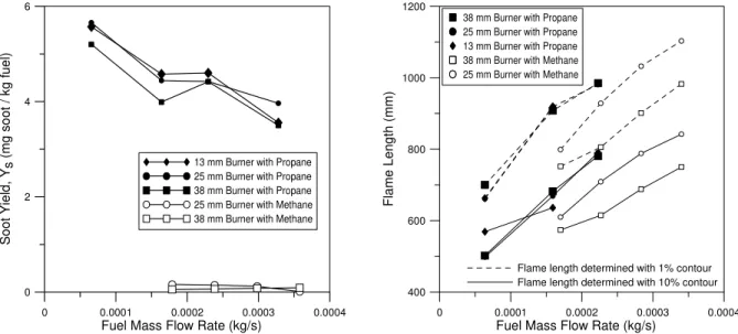
Soot emission rates and flame lengths were measured using different burner exit diameters and for a range of flow rates of either methane or propane (Figure 2). The soot yield data show that as would be expected there is a strong effect of fuel composition on soot yield and a secondary effect of fuel flow rate. By contrast, for the current range of experiments, there is no significant effect of burner diameter. As shown in Figure 2b, flame lengths grew linearly with fuel mass flow rate for the range of data collected. Flame lengths calculated using a 10% contour as

flame length is the critical parameter in estimating the residence as defined above, to permit an effective comparison with data in the literature, a flame contour was chosen so that the experimentally determined flame lengths in the current data matched those of Sivathanu [4] for an identical flow rate and burner diameter. Using available data for propane flames, a 1% contour produced flame lengths that matched those reported by Sivathanu [4].

0 0.0001 0.0002 0.0003 0.0004

Fuel Mass Flow Rate (kg/s)

0 2 4 6 So ot Yi e ld , Ys (mg so o t / kg fuel)

13 mm Burner with Propane 25 mm Burner with Propane 38 mm Burner with Propane 25 mm Burner with Methane 38 mm Burner with Methane

0 0.0001 0.0002 0.0003 0.0004

Fuel Mass Flow Rate (kg/s)

400 600 800 1000 1200 Fl a m e Len g th (mm)

38 mm Burner with Propane 25 mm Burner with Propane 13 mm Burner with Propane 38 mm Burner with Methane 25 mm Burner with Methane

Flame length determined with 1% contour Flame length determined with 10% contour

Figure 2: a) Measured soot yield for methane and propane using different burner exit diameters and flow rates and b) corresponding measured flame lengths

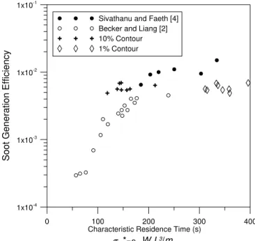
Figures 3 and 4 show the above results converted to a soot generation efficiency (SGE) and plotted as a function of characteristic residence time to allow a comparison with data from Becker and Liang [2] and Sivathanu [9]. It should be noted that all three authors have used a different technique for measuring soot concentration. Becker and Liang [2] used gravimetric sampling whereas Sivathanu and Faeth [3] used a laser extinction method. Since the 10% contour method calculated smaller flame lengths, it also produced smaller characteristic residence times, which can skew the data considerable as shown in Figure 3. With imposed matching flame lengths, the present data tends to follow the trend of Becker [2] and Sivathanu [9] for propane, although the logarithmic scale tends to minimize the data spread.

There is considerably more separation in the methane data as shown in Figure 4. In this case data plotted using a 10% flame length contour when calculating the residence time tend to agree better with Becker and Liang’s [2] data, however the relationship is not clear. The present data suggest a trend of increasing SGE up to a certain residence time after which SGE begins to decrease. Although Becker and Liang’s [2] methane data do not exhibit this same trend, other fuels they experimented with showed similar effects. A potential explanation for this disparity could be that that the residence time scaling laws change as buoyant jet flame conditions are reached which correspond to long characteristic residence times.

0 100 200 300 400 Characteristic Residence Time (s)

R*= W1L 3_/m 0 1x10-4 1x10-3 1x10-2 1x10-1 Soot G e n era tio n Efficiency

Sivathanu and Faeth [4] Becker and Liang [2] 10% Contour 1% Contour

Figure 3: Comparison of propane soot generation efficiency data with literature

40 80 120 160 200 240 280

Characteristic Residence Time (s)

R* W1L 3_/m 0 1x10-5 1x10-4 1x10-3 1x10-2 So ot G eneratio n E fficiency

Becker and Liang [2] 10% Contour 1% Contour

Figure 4: Comparison of methane soot generation efficiency data with literature

Another cause for discrepancies among the various data sets is the methods used for measuring soot concentration. The gravimetric method used by Becker and Liang [2] could be reaching the reproducibility and sensitivity limits with the low soot concentrations that are emitted from methane flames. Potential evidence to support this suggestion can be seen when comparing Figure 3 and 4. Becker and Liang [2] measure similar SGE’s for methane and propane whereas data from Trottier et al. [10] have shown an order-of-magnitude difference in the sooting propensities of propane and methane. Sivathanu and Faeth [3] estimate their soot volume

approximations and uncertainties in the refractive indices and the extinction method would also be limited at lower soot concentrations. Although the LII approach used in the present research is also susceptible to uncertainties in the refractive indices, considerable work has been completed since the publishing of Sivathanu and Faeth [3] that has reduced this uncertainty.

CONCLUSIONS

Soot mass emission rates of turbulent methane and propane diffusion flames were measured in a laboratory setting using laser-induced incandescence. Flame lengths were also measured using digital imaging to enable flame residence time calculations for comparison with published data of other researchers. Existing scaling relations based on buoyant flame residence times only partially describe the trends apparent in the soot yield data. These results highlight the subjective nature of flame length measurements and more data collected over a wider range of residence times will be required to draw firm conclusions. However, it is apparent from the comparison of current experiments and data in the literature that the residence time definition must be revisited if a suitable parameter is to be found to permit scaling of soot yield data from lab-scale flares to the industrial-scale flares.

ACKNOWLEDGEMENTS

This project is supported by the Canadian Association of Petroleum Producers (CAPP) and Environment Canada (Project Manager, Michael Layer).

REFERENCES

[1] J.H. Kent and S.J. Bastin, “Parametric Effects on Sooting in Turbulent Acetylene Diffusion Flames,” Combustion and Flame 56, pp. 29-42 (1984).

[2] H.A. Becker and D. Liang, “Total Emission of Soot and Thermal Radiation by Free Turbulent Diffusion Flames,” Combustion and Flame 44, pp. 305-318 (1982).

[3] Y.R. Sivathanu and G.M. Faeth, “Soot Volume Fractions in the Overfire Region of Turbulent Diffusion Flames,” Combustion and Flame 81, pp. 133-149 (1990).

[4] A. Coppalle and D. Joyeux, “Temperature and Soot Volume Fraction in Turbulent Diffusion Flames: Measurements of Mean and Fluctuating Values,” Combustion and Flame 96, pp. 275-285 (1994).

[5] The World Bank, (http://web.worldbank.org/), accessed March 21, 2007.

[6] G.R. Smallwood, W. Bachalo, and S. Sankar “Chapter 8 - Particulate Measurement Methods” In C. Mercer (Ed.), Optical Metrology for Fluids, Combustion, and Solids (pp. 221-257). Boston/Dordrecht/London: Kluwer Academic Publishers (2003).

[7] P. Canteenwalla, K.A. Thomson, G.J. Smallwood, and M.R. Johnson, “Sampling of Soot Emitted from Lab-scale Flares,” CI/CS Spring Technical Meeting, Waterloo, ON (2006).

[8] L.W. Kostiuk, A.J. Majeski, P.Poudenx, M.R. Johnson, and D.J. Wilson, “Scaling of Wake-Stabilized Jet Diffusion Flames in a Traverse Air Stream,” Proceedings of the Combustion Institute Vol. 28, pp. 553-559 (2000).

[9] Y.R. Sivathanu, personal communication – raw data from thesis (May 30, 2006).

[10] S. Trottier, H. Guo, G.J. Smallwood, and M.R. Johnson, “Measurement and Modeling of the Sooting Propensity of Binary Fuel Mixtures,” Proceedings of the International Combustion Symposium, Heidelberg, Germany (2006).