Bayesian nonparametric learning with semi-Markovian dynamics

Bayesian Nonparametric Learning with

semi-Markovian Dynamics

by

Matthew J Johnson

MASSACHUSETTS INSTITUTE OFTECHNOLOGY

JUL 12 2010

LIBRARIES

B.S. in Electrical Engineering and Computer Sciences

University of California at Berkeley, 2008

Submitted to the Department of Electrical Engineering and Computer

Science

in partial fulfillment of the requirements for the degree of

Master of Science in Electrical Engineering and Computer Science

at the

MASSACHUSETTS INSTITUTE OF TECHNOLOGY

June 2010

@

Massachusetts Institute of Technology 2010. All rights reserved.

Author

...

Department of Electrical Engineering anComputer Science

May 21, 2010

C ertified by ...

Edwin Sibley Webster Profes

I

Alan S. Willsky

sor of Electrical Engineering

Thesis Supervisor

A ccepted by ... ... .. ,...

Terry P. Orlando

Chairman, Department Committee on Graduate Students

Bayesian Nonparametric Learning with semi-Markovian

Dynamics

by

Matthew J Johnson

Submitted to the Department of Electrical Engineering and Computer Science on May 21, 2010, in partial fulfillment of the

requirements for the degree of

Master of Science in Electrical Engineering and Computer Science

Abstract

There is much interest in the Hierarchical Dirichlet Process Hidden Markov Model (HDP-HMM) as a natural Bayesian nonparametric extension of the ubiquitous Hidden Markov Model for learning from sequential and time-series data. However, in many settings the HDP-HMM's strict Markovian constraints are undesirable, particularly if we wish to learn or encode non-geometric state durations. We can extend the HDP-HMM to capture such structure by drawing upon explicit-duration semi-Markovianity, which has been developed in the parametric setting to allow construction of highly interpretable models that admit natural prior information on state durations.

In this thesis we introduce the explicit-duration Hierarchical Dirichlet Process Hid-den semi-Markov Model (HDP-HSMM) and develop posterior sampling algorithms for efficient inference. We also develop novel sampling inference for the Bayesian ver-sion of the classical explicit-duration Hidden semi-Markov Model. We demonstrate the utility of the HDP-HSMM and our inference methods on synthetic data as well as experiments on a speaker diarization problem and an example of learning the patterns in Morse code.

Thesis Supervisor: Alan S. Willsky

Contents

1 Introduction

2 Background 11

2.1 Bayesian Hidden Markov Models (HMMs) . . . . 11

2.1.1 M odel Specification . . . . 11

2.1.2 Posterior Inference via Gibbs Sampling . . . . 14

2.1.3 Sum m ary . . . . 17

2.2 Explicit-Duration Hidden Semi-Markov Models (HSMMs) . . . . 17

2.3 The Dirichlet Process . . . . 21

2.3.1 Defining the Dirichlet Process . . . . 21

2.3.2 Drawing Samples from a DP-distributed Measure . . . . 25

2.3.3 The Dirichlet Process Mixture Model . . . . 27

2.4 The Hierarchical Dirichlet Process . . . . 29

2.4.1 Defining the Hierarchical Dirichlet Process... . . .. 29

2.4.2 The Hierarchical Dirichlet Process Mixture Model . . . . 30

2.5 The Hierarchical Dirichlet Process Hidden Markov Model . . . . 32

3 New Models and Inference Methods 35 3.1 Sampling Inference in Finite Bayesian HSMMs . . . . 36

3.1.1 Outline of Gibbs Sampler . . . . 36

3.1.2 Blocked Conditional Sampling of (xt) with Message Passing . 37 3.1.3 Conditional Sampling of {r7} with Auxiliary Variables . . . . 38

3.2.1 Model Definition . . . . 42 3.2.2 _{Sampling Inference via Direct Assignments . . . .} 44 3.2.3 Sampling Inference with a Weak Limit Approximation . . . . 47

4 Experiments ₅₁

4.1 Synthetic D ata . . . . 52 4.2 Learning Morse Code . . . . 55 4.3 Speaker Diarization . . . . 58

5 Contributions and Future Directions 63

Chapter 1

Introduction

Given a set of sequential data in an unsupervised setting, we often aim to infer mean-ingful states, or "topics," present in the data along with characteristics that describe and distinguish those states. For example, in a speaker diarization (or who-spoke-when) problem, we are given a single audio recording of a meeting and wish to infer the number of speakers present, when they speak, and some characteristics governing their speech patterns [2]. In analyzing DNA sequences, we may want to identify and segment region types using prior knowledge about region length distributions [7,12]. Such learning problems for sequential data are pervasive, and so we would like to build general models that are both flexible enough to be applicable to many domains and expressive enough to encode the appropriate information.

Hidden Markov Models (HMMs) have proven to be excellent general models for approaching such learning problems in sequential data, but they have two significant disadvantages: (1) state duration distributions are necessarily restricted to a geomet-ric form that is not appropriate for many real-world data, and (2) the number of hidden states must be set a priori so that model complexity is not inferred from data in a Bayesian way.

Recent work in Bayesian nonparametrics has addressed the latter issue. In partic-ular, the Hierarchical Dirichlet Process HMM (HDP-HMM) has provided a powerful framework for inferring arbitrarily large state complexity from data

[14].

However, the HDP-HMM does not address the issue of non-Markovianity in real data. The

Markovian disadvantage is even compounded in the nonparametric setting, since non-Markovian behavior in data can lead to the creation of unnecessary extra states and unrealistically rapid switching dynamics [2].

One approach to avoiding the rapid-switching problem is the Sticky HDP-HMM [2], which introduces a learned self-transition bias to discourage rapid switching. In-deed, the Sticky model has demonstrated significant performance improvements over the HDP-HMM for several applications. However, it shares the HDP-HMM's restric-tion to geometric state durarestric-tions, thus limiting the model's expressiveness regarding duration structure. Moreover, its global self-transition bias is shared among all states, and so it does not allow for learning state-specific duration information. The infinite Hierarchical HMM

[5]

induces non-Markovian state durations at the coarser levels of its state hierarchy, but even the coarser levels are constrained to have a sum-of-geometrics form, and hence it can be difficult to incorporate prior information.

These potential improvements to the HDP-HMM motivate the investigation into explicit-duration semi-Markovianity, which has a history of success in the paramet-ric setting (e.g. [16]). In this thesis, we combine semi-Markovian ideas with the HDP-HMM to construct a general class of models that allow for both Bayesian non-parametric inference of state complexity as well as incorporation of general duration distributions. In addition, the sampling techniques we develop for the Hierarchical Dirichlet Process Hidden semi-Markov Model (HDP-HSMM) provide new approaches to inference in HDP-HMMs that can avoid some of the difficulties which result in slow

mixing rates.

The remainder of this thesis is organized as follows. In Chapter 2, we provide background information relevant to this thesis. In particular, we describe HMM modeling and the salient points of Bayesian learning and inference. We also provide a description of explicit-duration HSMMs and existing HSMM message-passing algo-rithms, which we use to build an efficient Bayesian inference algorithm in the sequel. Chapter 2 also provides background on the nonparametric priors and inference tech-niques we use to extend the classical HSMM: the Dirichlet Process, the Hierarchical Dirichlet Process, and the Hierarchical Dirichlet Process Hidden Markov Model.

In Chapter 3 we develop new models and inference methods. First, we develop a Gibbs sampling algorithm for inference in Bayesian constructions of finite HSMMs. Next, we describe the HDP-HSMM, which combines Bayesian nonparametric priors with semi-Markovian expressiveness. Finally, we develop efficient Gibbs sampling algorithms for inference in the HDP-HSMM, including both a collapsed sampler, in which we analytically marginalize over the nonparametric Dirichlet Process priors, and a practical approximate blocked sampler based on the standard weak-limit ap-proximation to the Dirichlet Process.

Chapter 4 demonstrates the effectiveness of the HDP-HSMM on both synthetic and real data using the blocked sampling inference algorithm. In synthetic exper-iments, we demonstrate that our sampler mixes very quickly on data generated by both HMMs and HSMMs and accurately learns parameter values and state cardinal-ity. We also show that while an HDP-HMM is unable to capture the statistics of an HSMM-generated sequence, we can build HDP-HSMMs that efficiently learn whether data were generated by an HMM or HSMM. Next, we present an experiment on Morse Code audio data, in which the HDP-HSMM is able to learn the correct state primi-tives while an HDP-HMM confuses short- and long-tone states because it is unable to incorporate duration information appropriately. Finally, we apply the HDP-HSMM to a speaker diarization problem, for which we achieve competitive performance and rapid mixing.

In Chapter 5 we conclude the thesis and discuss some avenues for future investi-gation.

Chapter 2

Background

2.1

Bayesian Hidden Markov Models (HMMs)

The Hidden Markov Model is a general model for sequential data. Due to its versatil-ity and tractabilversatil-ity, it has found wide application and is extensively treated in both textbooks, including [1], and tutorial papers, particularly [10]. This section provides

a brief introduction to the HMM, with emphasis on the Bayesian treatment.

2.1.1

Model Specification

The core of the HMM consists of two layers: a layer of hidden state variables and a layer of observation or emission variables. The relationships between the variables in both layers is summarized in the graphical model in Figure 2-1. Each layer consists of a sequence of random variables, and the indexing corresponds to the sequential aspect of the data (e.g. time indices).

The hidden state sequence, x

(xt)_

1 for some length T E N, is a sequence of

random variables on a finite alphabet, i.e. Xt

E

X = [N] A {1, 2, ... , N}, that forms

a Markov chain:

Vt E [T - 1] p(Xt+1 x1, x2,. . .,Xt) = p(xt+i|t). (2.1)

Figure 2-1: Basic graphical model for the HMM. Parameters for the transition, emis-sion, and initial state distributions are not shown as random variables, and thus this diagram is more appropriate for a Frequentist framework.

relevant history of the process in the sense that the future is statistically independent of the past given the present. It is the Markovian assumption that is at the heart of the simplicity of inference in the HMM: if the future were to depend on more than just the present, computations of interest would be more complex.

It is necessary to specify the conditional relationship between sequential hidden states via a transition distribution p(xt+1|xt, r), where 7r represents parameters of the conditional distribution. Since the states are taken to be discrete in an HMM (as opposed to, for example, a linear dynamical system), the transition distribution is usually multinomial and is often parameterized by a row-stochastic matrix 7r =

(rij)Hy 1 where 7rij = p(xt+1 = j'xt = i) and N is the a priori fixed number of possible states. The ith row gives a parameterization of the transition distribution out of state i, and so it is natural to think of r in terms of its rows:

71

r = .(2.2)

7rN

We also must specify an initial state distribution, p(X₁|7ro), where the 7ro parameter is often taken to be a vector directly encoding the initial state probabilities. We will use the notation {7ri}O to collect both the transition and initial state parameters into a single set, though we will often drop the explicit index set.

However, the variables do not form a Markov chain. In fact, there are no marginal in-dependence statements for the observation variables: the undirected graphical model that corresponds to marginalizing out the hidden state variables is fully connected. This result is a feature of the model: it is able to explain very complex statistical relationships in data, at least with respect to conditional independencies. However, the HMM requires that the observation variables be conditionally independent given the state sequence. More precisely, it requires

Vt

E

[T] yt 1 {y\t} U (X\t} |t (2.3) where the notation (y\t) denotes the sequence excluding the tth element, and a if b c

indicates random variables a and b are independent given random variable c. Given the corresponding state variable at the same time instant an observation is rendered independent from all other observations and states, and in that sense the state "fully explains" the observation.

One must specify the conditional relationship between the states and observations, i.e. p(ytlrt, 0), where 0 represents parameters of the emission distribution. These distributions can take many forms, particularly because the observations themselves can be taken from any (measurable) space. As a concrete example, one can take the example that the observation space is some Euclidean space R' for some k and the emission distributions are multidimensional Gaussians with parameters indexed by the state, i.e. in the usual Gaussian notation1_{, 0 } = {(i, Ei)}i}

1

.

With the preceding distributions defined, we can write the joint probability of the hidden states and observations in an HMM as

T-1 T

p((xt),

(yt)

{wi}, 0)

=

p(Xi

lwo)

P

p(xt+1|IX)1)

(

p(yt

1t|0) .

(2.4)

(t=1 ) t=1

The Bayesian and Frequentist formulations of the HMM diverge in their treatment of the parameters {i} and 0. A Frequentist framework would treat the parameters

'By usual Gaussian notation, we mean y is used to represent the mean parameter and E the

Figure 2-2: Basic graphical model for the Bayesian HMM. Parameters for the tran-sition, emission, and initial state distributions are random variables. The A and a symbols represent hyperparameters for the prior distributions on state-transition parameters and emission parameters, respectively.

as deterministic quantities to be estimated while a Bayesian framework would model them as random variables with prior distributions, which are themselves parameter-ized by hyperparameters. This thesis is concerned with utilizing a nonparametric Bayesian framework, and so we will use the Bayesian HMM formulation and treat parameters as random variables.

Thus we can write the joint probability of our Bayesian HMM as

p((xt), (yt), {7ri}, 0|a, A) = p(0|A)p({7ri}|a)p((xt), (yt)X{7ri}, 0) (2.5)

N T-1 T

=

H

p(6i|A)p({7ri}|a)p(xil7ro)

(fp(xt+1|xtJrr)

fJp(ytkxt|6)

i=1 t=1 t=1

(2.6)

for some observation parameter distribution p(0il A) and a prior on transitions p({7ri} A). A graphical model is given in Figure 2-2, where parameter random variables are shown in their own nodes. Hyperparameters are shown without nodes and assumed to be fixed and known a priori.

2.1.2

Posterior Inference via Gibbs Sampling

So far we have specified the HMM as a restricted class of probability distributions over sequences. From a practical standpoint, we are interested in the issues that arise when applying the model to data, i.e. finding some representation of the posterior

distribution over states and parameters when conditioning on the observations:

p((xt), 0, {7i} (yt), a, A). (2.7) We can perform posterior inference in the HMM with a Gibbs sampling algorithm, which allows us to construct samples from the posterior distribution by iteratively re-sampling some variables conditioned on their Markov blanket. We do not provide a general background for Gibbs sampling in this thesis, but the reader can find a thorough discussion in

[1].

An iteration of our Gibbs sampler samples the following conditional random vari-ables, which are ordered arbitrarily:

* (xt)|0, {7r}, (yt)

{wr,} a, 0, (Xt), (Yt) 0 1|A, (xt), (yt)

For example, when we sample the conditional random variable 0|A, (xt), (yt), that means we update the value of 0 to be a draw from its conditional distribution given the current values of A, (xt), yt. Sampling

{7}

and 0 from their conditional distributions is a standard problem which depends on the specific model distributions chosen; such issues are thoroughly described in, e.g.,

[1].

However, sampling (xt) is of particular importance and is not a standard procedure, and so we describe it in detail in the next section.

Block Sampling (xt)|6, {7r}, (yt) using Message Passing

To draw a conditional sample of the entire (xt) sequence at once, we exploit the Markov structure and use dynamic programming on the chain with the well-known "forwards-backwards" (or "alpha-beta") message passing algorithm for the HMM. We

define the messages as

(2.8) (2.9) (2.10)

at(Xt) p(yi, ... , y1, ot)

#3t(zt) Ap(yt+1, - . -, Yrlzt)

Or(XT) A1

where we have dropped the notation for conditioning on parameters 0 and

{w7}

for convenience. The at(xt) message is the probability of the data ending in state xt, and the /3t(xt) message is the probability of future data given a starting state of xt. We

also note that for any t we have

p(Xt yi, . . . , YT) OC at (Xt) 3,(Xt). (2.11)

The a and 3 messages can be which can be found in

[6]:

computed recursively through an easy derivation,

(2.12) (2.13) (2.14)

(2.15)

at

(zt+1)

= p

(Y1,

--. -,t+1, IXt+1)

= p

(yi,

. .. , ytIxt+1)p (Yt+1|I _t+1)p

(xt+1)

= p

(yi,

. .., yt I Op

(zt+1|

IXt)p (zt)p(yt+1| I

t+1)

Xt

Z

at (xt)P (xt+i

xt)p(yt~ilXt+i).

With similar manipulations, we can derive

(2.16)

Ot(Xt) = #3t(zt+1)p(zt+1|zt)P(yt+1|zt+1).

2t+1

Again, we have dropped the notation for explicitly conditioning on parameters. We can efficiently draw (xt) 0, {ri}, (yt) using only the 13 messages as follows.

t = 1, 2, ...,I T t = 1, 2, ...,I T - 1I

First, we note

p(zi

l0,

{7ri}, (yt)) ~c p(z1|{17i}p((yt)|Xi, 0, {7i}) (2.17)

= p(X11|7o)13 (Xi) (2.18)

and hence we can draw x,10,

{7rj},

(yt) by drawing from the normalized element-wise product of

#1

and wro. Supposing we draw x1 = x1, we can write

p(x2|0, {7j}, (yt), X1 oc X1) oc p(x2 |7i}, X1 = 21)p((Y2:T) X2, 0) (2.19)

p(X2|i = 21I, 7r21)#2(x2) (2.20)

and hence we can draw X2|0, {iri},

(yt),

X1 = x1 by drawing from the normalized

element-wise product of -rtl and /32. We can recurse this procedure to draw a block

sample of (xt) 0, {7r}, (yt).

2.1.3

Summary

In this section we have described the Bayesian treatment of the well-known Hidden Markov Model as well as the salient points of posterior inference with Gibbs sampling. There are two main disadvantages to the HMM that this thesis seeks to address simultaneously: the lack of explicit duration distributions and the issue of choosing the number of states from the data. The following background sections on Hidden semi-Markov Models and Bayesian nonparametric methods describe separate approaches to each of these two issues.

2.2

Explicit-Duration Hidden Semi-Markov

Mod-els (HSMMs)

There are several modeling approaches to semi-Markovianity [81, but here we focus on explicit duration semi-Markovianity; i.e., we are interested in the setting where each state's duration is given an explicit distribution.

Figure 2-3: A graphical model for the HSMM with explicit counter and finish nodes.

The basic idea underlying this HSMM formalism is to augment the generative process of a standard HMM with a random state duration time, drawn from some state-specific distribution when the state is entered. The state remains constant until the duration expires, at which point there is a Markov transition to a new state. It can be cumbersome to draw the process into a proper graphical model, but one compelling representation in [8] is to add explicit "timer" and "finish" variables, as depicted in Figure 2-3. The (Ct) variables serve to count the remaining duration times, and are deterministically decremented to zero. The (Ft) variables are binary-valued, F = 1 if and only if there is a Markov transition at time t + 1. Hence,

Ft = 1 causes Ct+1 to be sampled from the duration distribution of Xt+i, and the subsequent values Ct+2, Ct+3

,...

count down until reaching zero, at which point the

process repeats.

An equivalent and somewhat more intuitive picture is given in Figure 2-4 (which also appears in [8]), though the number of nodes in the model is itself random. In this picture, we see there is a standard Markov chain on "super-state" nodes, (zS)f 1,

and these super-states in turn emit random-length segments of observations, of which we observe the first T. The symbol Di is used to denote the random length of the observation segment of super-state i for i = 1,..., S. The "super-state" picture separates the Markovian transitions from the segment durations, and is helpful in building sampling techniques for the generalized models introduced in this thesis.

It is often taken as convention that state self-transitions should be ruled out in an HSMM, because if a state can self-transition then the duration distribution does not fully capture a state's possible duration length. We adopt this convention, which

Y1 YD1 YD1+1 YD1+D2 YT

Figure 2-4: HSMM interpreted as a Markov chain on a set of super-states, (z8) =1. The number of shaded nodes associated with each z, is random, drawn from a state-specific duration distribution.

has a significant impact on the inference algorithms described in Section 3. When defining an HSMM model, one must also choose whether the observation sequence ends exactly on a segment boundary or whether the observations are censored at the end, so that the final segment may possibly be cut off in the observations. This censoring convention allows for slightly simpler formulae and computations, and thus is adopted in this paper. We do, however, assume the observations begin on a segment boundary. For more details and alternative conventions, see [4].

It is possible to perform efficient message-passing inference along an HSMM state chain (conditioned on parameters and observations) in a way similar to the standard alpha-beta dynamic programming algorithm for standard HMMs. The "backwards" messages are crucial in the development of efficient sampling inference in Section 3 be-cause the message values can be used to efficiently compute the posterior information necessary to block-sample the hidden state sequence (xt), and so we briefly describe the relevant part of the existing HSMM message-passing algorithm. As derived in [8], we can define and compute the backwards message from t to t

+

1 as follows:

it(i) AP(Yt+1:lt = iF 1) (2.21) = Ot(jAp(zt+1 = I zt = i) (2.22) St()Ap(yt+1:r

lzt+1

i F = 1) (2.23) T-t

S/

3 t+d(i) p(Dt+ i) p(yt+1:t+dXt+1 i, Dt+1 d) (2.24)

d=1 duration prior term likelihood term

+ p(Dt+1 > T - txt+i = i)P(Yt+1:TlXt+1= i, Dt+1 > T - t) (2.25)

censoring term

O (i) A1 (2.26)

where we have split the messages into

#

and 3* components for convenience and used Yki:k2 to denote (Yk,. .. , Yk2). Also note that we have used Dt+1 to represent the duration of the segment beginning at time t

+

1. The conditioning on the parameters of the distributions is suppressed from the notation. This backwards message-passing recursion is similar to that of the HMM, and we will find that we can use the values

of P(Yt+1:TXt i, F = 1) for each possible state i in the efficient forward-sampling algorithm of Section 3.

The F= 1 condition indicates a new segment begins at t

+

1, and so to compute the message from t+ 1 to t we sum over all possible lengths d for the segment beginning at t

+

1, using the backwards message at t

+

d to provide aggregate future information

given a boundary just after t

+

d. The final additive term in the expression for Ot* (i)

is described in

[4];

it constitutes the contribution of state segments that run off the end of the provided observations, as per the censoring assumption, and depends on the survival function of the duration distribution.

This message passing algorithm will be a subroutine in our Gibbs sampling al-gorithm; more specifically, it will be a step in block-resampling the state sequence (xt) from its posterior distribution. Though a very similar technique is used in HMM Gibbs samplers, it is important to note the significant differences in computational

cost between the HMM and HSMM message computations. The greater expressiv-ity of the HSMM model necessarily increases the computational cost of the message passing algorithm: the above message passing requires O(T 2N

+

TN2_{) basic}

opera-tions for a chain of length T and state cardinality N, while the corresponding HMM message passing algorithm requires only O(TN2). However, if we truncate possible

segment lengths included in the inference messages to some maximum dmax, we can in-stead express the asymptotic message passing cost as O(TdmaxN2). Such truncations

are often natural because both the duration prior term and the segment likelihood term contribute to the product rapidly vanishing with sufficiently large d. Though the increased complexity of message-passing over an HMM significantly increases the cost per iteration of sampling inference for a global model, the cost is offset because HSMM samplers often need far fewer total iterations to converge (see Section 3).

Bayesian inference in an HDP-HSMM via Gibbs sampling is a novel contribution of this thesis, and it is discussed in Section 3.1.

2.3

The Dirichlet Process

The Dirichlet Process is a random process that has found considerable use as a prior in Bayesian nonparametrics. It is an extension of the Dirichlet distribution to general measurable spaces, and it possesses several desirable properties. In particular, it describes a distribution over infinitely many "clusters" or "topics," allowing us to infer and mix over arbitrary degrees of model complexity that grow with the amount of data.

In this section, we define the Dirichlet Process, outline its properties, and describe statistical inference procedures based on sampling. We also describe the prototypical Dirichlet Process Mixture Model.

2.3.1

Defining the Dirichlet Process

Definition (Implicit) Let (Q, B) be a measurable space, H be a probability mea-sure on that space, and ozo be a positive real number. A Dirichlet Process (DP) is

the distribution of a random probability measure G over (Q, B) if and only if for any finite (disjoint) partition (A1,... , A,) of Q we have

(G(A1), ... , G(Ar)) ~ Dir(aoH(A1), ... , aoH(A,)) (2.27)

where Dir denotes the standard Dirichlet distribution. We write G ~ DP(cao, H) and call ao the concentration parameter and H the base measure

[13].

Note that the preceding definition is implicit rather than constructive. However, it implies the following properties:

Property 1. E[G(A)] = H(A) VA E B. This property follows immediately from the expectation properties of the standard Dirichlet distribution.

Property 2. If we have samples {O2}Yi drawn according to

G|H, ao ~ DP(H, ao) (2.28)

O6|G ~ G i = 1,. .. ,N, (2.29) i.e., we draw a random probability measure G from a Dirichlet Process and then draw samples

{6O}

from G, then we have

(G(A 1), ... , G(Ar)) 01,. . ., -~ Dir(aoH(A1) + N1,... , aoH(A,) + N,) (2.30)

for any partition, where Nk counts the number of samples that fall into partition element k. This property follows from the standard Dirichlet conjugacy [13].

Property 3. Since each Ak partition element can be arbitrarily small around some O6 that falls into it, we note that the posterior must have atoms at the observed {O} values. Furthermore, by conjugacy it still respects the same finite partition Dirichlet

property as in the definition, and so the posterior is also a DP:

G|{;}, ao,H~DP (o±+E nka+N (aoH + 60 ) (2.31) where 60, represents an atom at O6.

Property 4.

im E[G(T)|{6O},ao,H] = Z76,(T) (2.32)

N-oo

k

wheref

{#}

are the distinct values of {O} and ikA limN-o Nk. This property follows from noting that, due to Property 3, the atomic empirical measure component grows in total mass compared to the base measure in the posterior parameter, and since the expectation of a DP is equivalent in measure to its parameter (i.e., if G ~ DP(H, ao) then E[G(A)] = H(A) for any measurable A), we have that the expectation of the posterior must go to the empirical distribution in the limit.

Property 5. G ~ DP(ao, H) is discrete almost surely. This result is stated without

justification here, but it is described in [13).

These properties, which are derived directly from the implicit definition, already illuminate several desirable properties about the DP: namely, its relationship to the standard Dirichlet distribution (but with more general conjugacy), its consistency in the sense that it is clear how the posterior converges to the empirical distribution, and the fact that draws from a DP are discrete with probability 1. Furthermore, we can also see the reinforcement property in which more common samples increasingly dominate the posterior. However, while several properties are apparent, the preceding definition is implicit and does not inform us how to construct a sample G distributed according to G H, ao ~ DP(H, ao).

There is a constructive definition of the Dirichlet Process, which is equivalent with probability 1, referred to as the stick breaking construction. First, we define a stick

breaking process with parameter ao as

Pk

lao

~Beta(1, ao) k = 1,2, ... (2.33)

k-1

/3k PkH (1 - pe). (2.34)

f=1

For a definition of the Beta distribution, see [1]. To describe this process we write simply - GEM(ao). The preceding is referred to as a stick breaking process because

it can be visualized as breaking a stick of unit length into pieces, with each piece a Beta(1, ao) proportion of the remaining length. We can then use these weights to construct G ~ DP(H, ao) [3]:

OkH ~H k = 1,2, ... (2.35)

c

3k 1 60, (2.36)

k=1

where 6_{0, represents an atom at} 0_{k. To summarize, we have the following definition:}

Definition (Stick Breaking) Let (w, B) be a measurable space, H be a probability

measure on that space, and ao be a positive real number. A Dirichlet Process is the distribution of a random probability measure G constructed as

#|ao

~ GEM(ao) (2.37)

OklH ~ H k = 1,2, ... (2.38)

G E Z3k6o0. (2.39)

k=1

The stick breaking construction of a Dirichlet Process draw provides an alternative parameterization of the DP in terms of unique atom components. This parameteri-zation can be useful not only to explicitly construct a measure drawn from a DP, but also in the design of sampling procedures which marginalize over G, as we discuss in the next section.

2.3.2

Drawing Samples from a DP-distributed Measure

We can draw samples from a measure G distributed according to the Dirichlet Process

without instantiating the measure itself. That is, we can generate samples {2} that are distributed as

G H, ao ~ DP(H, ao) (2.40)

BilG ~ G i = 1, ...,I N (2.41)

where we effectively marginalize out G. Using the posterior properties described previously, we can consider the predictive distributions on samples when we integrate out the measure G [13]:

P(ON+1 E Al01, ... ,ON) = E [G(A)|61, ... ION] (2.42)

I N

ao+ N aoH(A) + o60i) (2.43)

The final line describes a Polya urn scheme [13] and thus allows us to draw samples

from a Dirichlet process. First, we draw 011H - H. To draw i+1|01,.... , Oi, H,

we choose to sample a new value with probability ', in which case we draw

±i+1|01,..- , O. , H ~ H, or we choose to set i+1 = 0, for all

j

= 1,... , i with equal

probability 1. This Polya urn procedure will generate samples as if they were drawn from a measure drawn from a Dirichlet Process, but clearly we do not need to directly instantiate all or part of the (infinite) measure.

However, the Polya urn process is not used in practice because it exhibits very slow mixing rates in typical models. This issue is a consequence of the fact that there may be repeated values in the

{0;},

leading to fewer conditional independencies in the model.

We can derive another sampling scheme that avoids the repeated-value problem by following the stick breaking construction's parameterization of the Dirichlet Pro-cess. In particular, we examine predictive distributions for both a label sequence,

{

z 1}i>, and a sequence of distinct atom locations, {OkkI1. We equivalently write

our sampling scheme for

{O}

as:

#|ao ~ GEM(ao) (2.44)

OkH ~ H k = 1,2,... (2.45)

z i = 1, 2,..., N (2.46)

S 2, i =1, 2, ... , N (2.47)

where we have interpreted 3 to be a measure over the natural numbers.

If we examine the predictive distribution on the labels {zi}, marginalizing out 3,

we arrive at a description of the Chinese Restaurant Process (CRP)

[13].

First, we set

zi = 1, representing the first customer sitting at its own table, in the language of the

CRP. When the (i

+

1)th customer enters the restaurant (equivalently, when we want to draw zi+1 zi,..., zi), it sits at a table proportional to the number of customers

already at that table or starts its own table with probability '0 . That is, if the first i customers occupy K tables labeled as 1, 2, ... , K, then

1

k

k

1,2

...

_{. K}

p(zi+1 = k) = o+ (2.48)

where Nk denotes the number of customers at table k, i.e. Nk 1 [z = k].

Each table is served a dish sampled i.i.d. from the prior, i.e. O6jH ~ H, and all customers at the table share the dish.

The Chinese Restaurant Process seems very similar to the Polya urn process, but since we separate the labels from the parameter values, we have2 _{that O _LL O6 if}

zi f zj. In terms of sampling inference, this parameterization allows us to re-sample

entire tables (or components) at a time by re-sampling 6 variables, whereas with the Polya urn procedure the O6 for each data point had to be moved independently.

2

For this independence statement we also need H such that O6 # Oj a.s. for i / j, i.e. that independent draws from H yield distinct values with probability 1.

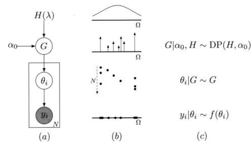
H(A)

a

G

JtA

t

Glao,

H

~DP(H,

ao)

61 N. ei I|G ~G

yi|6 ~

f

(00 N

(a) (b) (C)

Figure 2-5: Dirichlet Process Mixture Model: (a) graphical model, where the obser-vation nodes are shaded; (b) depiction of sampled objects in the DPMM; (c) corre-sponding generative process.

2.3.3 The Dirichlet Process Mixture Model

We can construct a DP Mixture Model

(DPMM)

much as we construct a standard Dirichlet mixture model [1], except if we use the Dirichlet process as the prior over both component labels and parameter values we can describe an arbitrary, potentially

infinite number of components.

We can write the generative process for the standard DPMM as

GH, ao ~ DP(H, ao) (2.49)

BilG ~ G i = 1, 2, . .. , N (2.50)

yFigu ~ f (c) ie= 1, 2, .M.o. , N (2.51)

where

f

is a class of observation distributions parameterized by D. The graphical

model for the DPMM is given in Figure 2-5(a). For concreteness, we may consider

f

to be the class of scalar, unit-variance normal distributions with a mean parameter, i.e.

f(i)

= r(ir, 1). The measure H could then be chosen to be the conjugate prior,

also a normal distribution, with hyperparameters A = (po, o anPossible samples from this setting are sketched in Figure 2-5(b).

keeping track of the label random variables {zk}:

#|ao ~ GEM(ao) (2.52)

Ok H ~ H k = 1, 2, ... (2.53)

zil3 i = 1,2, ... , N (2.54)

y zi, {Ok} f (O2).i 1,2, ... , N (2.55)

A graphical model is given in Figure 2-6.

To perform posterior inference in the model given a set of observations

{y}

K1, we

are most interested in conditionally sampling the label sequence {zi}. If we choose our observation distribution

f

and the prior over its parameters H to be a conjugate pair, we can generally represent the posterior of

{Ok}K

1 {yJ} 1, {z}N 1, H in closed form,

where K counts the number of unique labels in {zi} (i.e., the number of components present in our model for a fixed {zi}). Hence, our primary goal is to be able to re-sample {zi}|{yi}, H, ao, marginalizing out the

{Ok}

parameters.

We can create a Gibbs sampler to draw such samples by following the Chinese Restaurant Process. We iteratively draw ziI{z\i},

{yi},

H, ao, where {z\i} denotes all other labels, i.e. {zj :

j

f i}. To re-sample the ith label, we exploit the exchange-ability of the process and consider zi to be the last customer to enter the restaurant. We then draw its label according to

p(zi = k) oc

Nkf (yil{yj : zy =

k})

k = 1,

2,...,

K

(2.56)

ao k=K+1

where K counts the number of unique labels in {z\i} and

f(yil{yy

: z= k}) repre-sents the predictive likelihood of yi given the other observation values with label k, integrating out the table's parameter 0_{k. This process both instantiates and deletes}

Figure 2-6: Alternative graphical model for the DPMM, corresponding to the stick breaking parameterization. The observation nodes are again shaded.

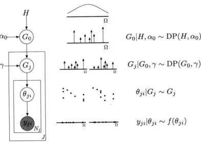
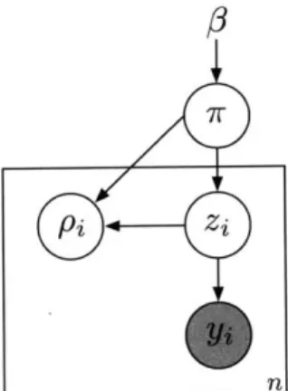
2.4

The Hierarchical Dirichlet Process

The Hierarchical Dirichlet Process (HDP) is a hierarchical extension of the Dirichlet Process which constructs a set of dependent DPs. Specifically, the dependent DPs share atom locations and have similar, but not identical, weights on their correspond-ing atoms. As described in this section, such a set of Dirichlet Processes allows us to build a Bayesian nonparametric extension of the Hidden Markov Model with the same desirable model-order inference properties as seen in the Dirichlet Process Mixture Model.

2.4.1

Defining the Hierarchical Dirichlet Process

Definition Let H be a probability measure over a space (Q, B) and ao and y be positive real number. We say the set of probability measure

{Gj}j_1

are distributed according to the Hierarchical Dirichlet Process if

Go H, ao ~ DP(H, ao) (2.57)

Gi|Go, -y ~ D P(Go, -y) j = 1, 2,1. .. , J (2.58) (2.59)

for some positive integer J which is fixed a priori.

Note that by Property 1 of the Dirichlet Process, we have E[Gy(A)IGo] = Go(A)

distribution shared by the dependent DPs. The y parameter is an additional concen-tration parameter, which controls the dispersion of the dependent DPs around their mean. Furthermore, note that since Go is discrete with probability 1, Gj is discrete with the same set of atoms.

There is also a stick breaking representation of the Hierarchical Dirichlet Process:

Definition (Stick Breaking) We say {Gj_1 are distributed according to a Hi-erarchical Dirichlet Process with base measure H and positive real concentration parameters ao and 7y if 03|ao ~ GEM(ao) (2.60) OkH ~ H k = 1, 2, ... (2.61) 00

Go

Oko66 (2.62) k=1 (2.63) iryl~y ~ GEM(7-) j=1, 2, . .. , J (2.64) |Go ~ Go i=1,2, . . . , Ny (2.65) 00 Gy Z ji 60o. (2.66) i=1

Here, we have used the notation 6k to identify the distinct atom locations; the OB7 are non-distinct with positive probability, since they are drawn from a discrete measure. Similarly, note that we use igi to note that these are the weights corresponding to the non-distinct atom locations 0ji; the total mass at that location may be a sum of several iii.

2.4.2

The Hierarchical Dirichlet Process Mixture Model

In this section, we briefly describe a mixture model based on the Hierarchical Dirichlet Process. The Hierarchical Dirichlet Process Mixture Model (HDPMM) expresses a set of J separate mixture models which share properties according to the HDP.

n n n Go I H, ao ~ DP(H, ao) GIGo, y ~ DP(Go, 7) Oj|Gj ~ Gj yg|6 j ~ f (69)

Figure 2-7: The Hierarchical Dirichlet Process Mixture Model: (a) graphical model; (b) depiction of sampled objects; (c) generative process.

Specifically, each mixture model is parameterized by one of the dependent Dirichlet Processes, and so the models share mixture components and are encouraged to have similar weights.

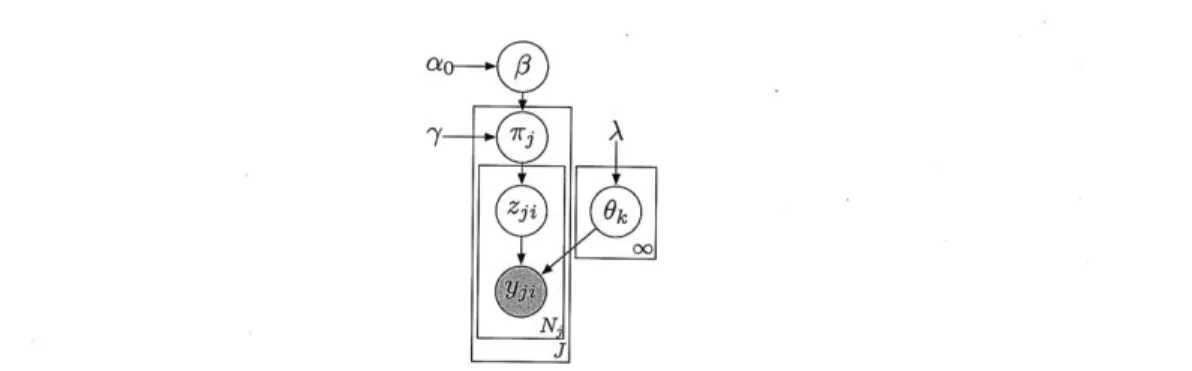
One parameterization of the HDPMM is summarized in Figure 2-7. However, the parameterization that is most tractable for inference follows the stick breaking construction but eliminates the redundancy in the parameters:

O|ao D 7ry|, 10 ~ D zgf/3ry ~Dry OkH ~H Yjil(Ok}, zji f ( P(1, ao) P(3, 7) k = 1, 2,... 62)

This third parameterization of the HDP is equivalent [3] to the other parameteri-zations, and recovers the distinct values3 _{of the {Ok} parameters while providing a}

label sequence {z3i} that is convenient for resampling. A graphical model for this parameterization of the mixture model is given in Figure 2-8.

3

Here we have assumed that H is such that two independent draws are distinct almost surely. This assumption is standard and allows for this convenient reparameterization.

(2.67) (2.68) (2.69) (2.70) (2.71)

j

= 1, 2,1. .. , J i = 1, 2, . . ., Nj

Figure 2-8: A graphical model for the stick breaking parameterization of the Hierar-chical Dirichlet Process Mixture Model with unique atom locations.

To perform posterior inference in this mixture model, there are several sampling schemes based on a generalization of the Chinese Restaurant Process, the Chinese Restaurant Franchise. A thorough discussion of these schemes can be found in [14].

2.5

The Hierarchical Dirichlet Process Hidden Markov

Model

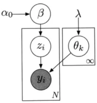
The HDP-HMM [14] provides a natural Bayesian nonparametric treatment of the clas-sical Hidden Markov Model approach to sequential statistical modeling. The model employs an HDP prior over an infinite state space, which enables both inference of state complexity and Bayesian mixing over models of varying complexity. Thus the HDP-HMM subsumes the usual model selection problem, replacing other techniques for choosing a fixed number of HMM states such as cross-validation procedures, which can be computationally expensive and restrictive. Furthermore, the HDP-HMM in-herits many of the desirable properties of the HDP prior, especially the ability to encourage model parsimony while allowing complexity to grow with the number of observations. We provide a brief overview of the HDP-HMM model and relevant inference techniques, which we extend to develop the HDP-HSMM.

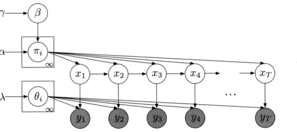
Figure 2-9: Graphical model for the HDP-HMM.

The generative HDP-HMM model (Figure 2-9) can be summarized as:

3_{|y ~ GEM(y) (2.72)}

7rj 1#, a ~ DP(a,,#) j = 1,2 ... (2.73)

0j|H, A ~ H(A) j = 1,2, ... (2.74)

41|7r0}1, zt_1 ~ 72,, t = 1, . .. ,IT (2.75)

yt{} Oi0Xt ~

f

(O6t) t = 1, ... , T (2.76)

where GEM denotes a stick breaking process [11]. We define /r Fro to be a separate

distribution.

The variable sequence (Xt) represents the hidden state sequence, and (yt) repre-sents the observation sequence drawn from the observation distribution class

f.

The set of state-specific observation distribution parameters is represented by

{

6}, which are draws from the prior H parameterized by A. The HDP plays the role of a prior over infinite transition matrices: each iry is a DP draw and is interpreted as the transition distribution from state

j,

i.e. the jth row of the transition matrix. The 7rj are linked by being DP draws parameterized by the same discrete measure 3, thus E[7r] = 0 and the transition distributions tend to have their mass concentrated around a typical set of states, providing the desired bias towards re-entering and re-using a consistent set of states.

ap-proximate inference for the full infinite-dimensional HDP, but they have a particular weakness in the context of the HDP-HMM: each state transition must be re-sampled individually, and strong correlations within the state sequence significantly reduce mixing rates for such operations [3]. As a result, finite approximations to the HDP have been studied for the purpose of providing alternative approximate inference schemes. Of particular note is the popular weak limit approximation, used in [2], which has been shown to reduce mixing times for HDP-HMM inference while sacri-ficing little of the "tail" of the infinite transition matrix. In this thesis, we describe how the HDP-HSMM with geometric durations can provide an HDP-HMM sampling inference algorithm that maintains the "full" infinite-dimensional sampling process while mitigating the detrimental mixing effects due to the strong correlations in the state sequence, thus providing a novel alternative to existing HDP-HMM sampling methods.

Chapter 3

New Models and Inference

Methods

In this chapter we develop new models and sampling inference methods that extend the Bayesian nonparametric approaches to sequential data modeling.

First, we develop a blocked Gibbs sampling scheme for finite Bayesian Hidden semi-Markov Models; Bayesian inference in such models has not been developed pre-viously. We show that a naive application of HMM sampling techniques is not possible for the HSMM because the standard prior distributions are no longer conjugate, and we develop an auxiliary variable Gibbs sampler that effectively recovers conjugacy and provides very efficient, accurate inference. Our algorithm is of interest not only to provide Bayesian sampling inference for the finite HSMM, but also to serve as a sampler in the weak-limit approximation to the nonparametric extensions.

Next, we define the nonparametric Hierarchical Dirichlet Process Hidden semi-Markov Model (HDP-HSMM) and develop a Gibbs sampling algorithm based on the Chinese Restaurant Franchise sampling techniques used for posterior inference in the HDP-HMM. As in the finite case, issues of conjugacy require careful treatment, and we show how to employ latent history sampling [9] to provide clean and efficient Gibbs sampling updates. Finally, we describe a more efficient approximate sampling inference scheme for the HDP-HSMM based on a common finite approximation to the HDP, which connects the sampling inference techniques for finite HSMMs to the

Bayesian nonparametric theory.

The inference algorithms developed in this chapter not only provide for efficient inference in the HDP-HSMM and Bayesian HSMM, but also contribute a new proce-dure for inference in HDP-HMMs.

3.1

Sampling Inference in Finite Bayesian HSMMs

In this section, we develop a sampling algorithm to perform Bayesian inference in finite HSMMs. The existing literature on HSMMs deals primarily with Frequentist formulations, in which parameter learning is performed by applications of the Ex-pectation Maximization algorithm [1]. Our sampling algorithm for finite HSMMs contributes a Bayesian alternative to existing methods.

3.1.1

Outline of Gibbs Sampler

To perform posterior inference in a finite Bayesian Hidden semi-Markov model (as defined in Section 2.2), we can construct a Gibbs sampler resembling the sampler described for finite HMMs in Section 2.1.2.

Our goal is to construct a particle representation of the posterior

p((xt), 0, {7},

{

wi}(yt), a-, A) (3.1) by drawing samples from the distribution. This posterior is comparable to the pos-terior we sought in the Bayesian HMM formulation of Eq. 2.7, but note that in the HSMM case we include the duration distribution parameters, {w}. We can construct these samples by following a Gibbs sampling algorithm in which we iteratively sample

from the distributions of the conditional random variables:

(Xt) 0, {7ri}, {w}, (Yt) (3.2)

{7i}|a, (zt) (3.3)

{wi}|(zt), T1 (3.4)

0 A, (Xt), (Yt) (3.5)

where r/ represents the hyperparameters for the priors over the duration parameters

{wi}.

Sampling 0 or {wi} from their respective conditional distributions can be easily reduced to standard problems depending on the particular priors chosen, and further discussion for common cases can be found in

[1].

However, sampling (xt)|0,

{7rj,

(yt)

and

{7ri}|a,

(xt) in a Hidden semi-Markov Model has not been previously developed. In the following sections, we develop (1) an algorithm for block-sampling the state sequence (xt) from its conditional distribution by employing the HSMM message-passing scheme of Section 2.2 and (2) an auxiliary variable sampler to provide easily resampling of

{7r}

from its conditional distribution.

3.1.2 Blocked Conditional Sampling of (Xt) with Message

Pass-ing

To block sample (Xt) 0, {7ri},

{wi},

(yt) in an HSMM we can extend the standard block

state sampling scheme for an HMM, as described in Section 2.1.2. The key challenge is that to block sample the states in an HSMM we must also be able to sample the posterior duration variables.

If we compute the backwards messages

Q

and 0* described in Section 2.2, then we can easily draw a posterior sample for the first state according to:

p(Xi = yi:T) OC p(zi =i)P(Yi:Ti =, FO = 1) (3.6)

where we have used the assumption that the observation sequence begins on a segment boundary (Fo = 1) and suppressed notation for conditioning on parameters. This first step is directly analogous to the first step of sampling (Xt) for an HMM.

We can also use the messages to efficiently draw a sample from the posterior dura-tion distribudura-tion for the sampled initial state. Condidura-tioning on the initial state draw, 21, we can draw a sample of D1|Y1:T, x1 = 21 (suppressing notation for conditioning

on parameters), the posterior duration of the first state is:

p(D1 = dlYi:T, X1 = ±1, FO = 1) =P(D₁ d)Yi:tIXi XiFo) (2) p(yi:tlxi = x1, FO)

_ P(D ₁ = dlzi x ,= 2 FO)P(Yl:d D₁ = d, Q1, FO)P(Yd+1:t D₁ = d, xi = 21, Fo) (3.8)

p(yi:t li = i, Fo)

_ p(Di = d)p(Yl:d|Dl = d, x1 = t₁, Fo = 1)#3d(2t1) (39)

130 (21)

We can repeat the process by then considering XD₁+1 to be our new initial state with initial distribution given by p(XD1+1 i 1 =t1), analogous to the HMM case.

3.1.3

Conditional Sampling of {7r} with Auxiliary Variables

In the standard construction of an HSMM, as described in Section 2.2, self-transitions are ruled out. However, in the Bayesian setting, this restriction means that the Dirichlet distribution is not a conjugate prior for the transition parameters,

{rs},

as it is in the Bayesian HMM construction.

To observe the loss of conjugacy, note that we can summarize the relevant portion of the generative model as

j7l--Dir(/31,...,a#L) j=1,...,L

t{7r , e t with te1 1

t = 2, ... I

T

appropri-ately, i.e.:

rc -

)ij

L

-11

with 6oj = 1 if i

j

and

osj

= 0 otherwise. The deterministic transformation from

iry to frJ eliminates self-transitions. Note that we have suppressed the observation

parameter set, duration parameter set, and observation sequence sampling for sim-plicity.

Consider the distribution of 1kri(xt), 3:

p(71| (xt), 3) oc p(7r1|i)p((xt) |71)

D -1 2-1 . -1 712 1 2 71 3 n .'.. 7i _

1 g

1 1 rii _{1 7r1 1 - 711}

where nij are the number of transitions from state i to state

j

in the state sequence

(xt). Essentially, because of the extra 1 terms from the likelihood without

self-transitions, we cannot reduce this expression to the Dirichlet form over the compo-nents of r1.

However, we can introduce auxiliary variables to recover conjugacy. For notational convenience, we consider the simplified model:

-Fr|# ~ Dir(O)

zil -r ~ Zr = 1,..) n

yilzi ~ f (zi) i = 1, .* , n

where ir is formed by removing the first component of -r and re-normalizing. Here, the

{zi}

directly represent the multinomial transitions of the state sequence (xt), and the

{yi}

embody the effect of the observation sequence (yt). See the graphical model in Figure 3-1 for a depiction of the relationship between the variables.

Figure 3-1: Simplified depiction of the relationship between the auxiliary variables and the rest of the model.

between drawing {zi} 7r, {yi} and

wjr{zi},

but as before the latter step is difficult because we do not have a conjugate Dirichlet distribution over 7r:

p(7r|{z1}) cx r 3lr2#2-1 .. .7r

OL

1)r

(

2

(

3

)n3

...

(

T

U L)

P(7rfzi) () -X 21 - 71 1-7 (ri1 - 7ri

However, we can introduce the auxiliary variables {pi}_ 1, where each pi is

inde-pendently drawn from a geometric distribution supported on

{0,

1, ...

}

with success

parameter 1 - 7ri, i.e. pi - Geo(1 - 7ri). Thus our posterior becomes:

p(7r|{zi}, {pi}) c p(7r)p({zi} 7r)p({pi}|{7ri})

0C7)1-1 702-1 . F)L-1 2 n 73 n3... L n n7Pi r)

1+Z ip-1 32+n2-1 . L+fL-1

7 72 .. FL

oc Dir(31 + p ,#2 + n2, ... ,#L + nL)

and so, noting that n = ni, we recover conjugacy.

Intuitively, we are able to fill in the data to include self-transitions because before each transition is sampled, we must sample and reject Geo(1 - 7ri) self-transitions. Note that this procedure depends on the fact that, by construction, the {pi} are conditionally independent of the data, {yi}, given {zi}.

t1 I t2 =D1+1 ts =T-Ds +1 t'=D1 t' = D1+D2 t's =T

Figure 3-2: Graphical model for the weak-limit approximation including auxiliary variables.

completed the data with the auxiliary variables, we are once again in the conjugate setting and can use standard sampling methods. A graphical model for a finite HSMM including the auxiliary variables is shown in Figure 3-2. Note that each pti depends on the state label Xt. _{Also note that Figure 3-2 draws the parameters 3 and}

_{7ri}

as coupled according to the weak limit approximation, which will be discussed in Section 3.2.3.

3.2

_{The Hierarchical Dirichlet Process Hidden}

Semi-Markov Model

In this section we introduce the Hierarchical Dirichlet Process Hidden semi-Markov Model (HDP-HSMM), the nonparametric extension of the finite HSMM, and develop efficient inference techniques.