Establishing damage criteria for multi-year ice phase I : thickness and temperature of drifting floes

(1)

Publisher’s version / Version de l'éditeur:

Vous avez des questions? Nous pouvons vous aider. Pour communiquer directement avec un auteur, consultez la première page de la revue dans laquelle son article a été publié afin de trouver ses coordonnées. Si vous n’arrivez pas à les repérer, communiquez avec nous à PublicationsArchive-ArchivesPublications@nrc-cnrc.gc.ca.

Questions? Contact the NRC Publications Archive team at

PublicationsArchive-ArchivesPublications@nrc-cnrc.gc.ca. If you wish to email the authors directly, please see the first page of the publication for their contact information.

https://publications-cnrc.canada.ca/fra/droits

L’accès à ce site Web et l’utilisation de son contenu sont assujettis aux conditions présentées dans le site LISEZ CES CONDITIONS ATTENTIVEMENT AVANT D’UTILISER CE SITE WEB.

Technical Report; no. CHC-TR-066, 2009-03-01

READ THESE TERMS AND CONDITIONS CAREFULLY BEFORE USING THIS WEBSITE. https://nrc-publications.canada.ca/eng/copyright

NRC Publications Archive Record / Notice des Archives des publications du CNRC :

https://nrc-publications.canada.ca/eng/view/object/?id=f3e0d369-d3de-4de4-8264-8a626d284d53 https://publications-cnrc.canada.ca/fra/voir/objet/?id=f3e0d369-d3de-4de4-8264-8a626d284d53

For the publisher’s version, please access the DOI link below./ Pour consulter la version de l’éditeur, utilisez le lien DOI ci-dessous.

https://doi.org/10.4224/20178995

Access and use of this website and the material on it are subject to the Terms and Conditions set forth at

Establishing damage criteria for multi-year ice phase I : thickness and temperature of drifting floes

(2)

Establishing Damage Criteria for Multi-year Ice

Phase I: Thickness and Temperature of Drifting Floes

M. Johnston

31 May 23 Jul 1 Aug 13 Aug 17 Aug 25 Aug 2 Sep 7 Sep 20 Sep Parry Channel M’Clintock Channel Wellington Channel Austin Channel Resolute H 21 1 25 26 27 28 29 30 31 32 33353637 3839 34 24 22 23 2 3 4 5 6 7 8 9 10 11 12 13 14 15 16 17 18 20 Transect 1 Transect 2 Transect 3 Transect 4 Transect 5 Transect 6 temperature chain drill hole thicknesses

Technical Report, CHC-TR-066

March 2009

(3)

(4)

Establishing Damage Criteria for Multi-year Ice, Phase I:

Thickness and Temperature of Drifting Floes

M. Johnston

Canadian Hydraulics Centre National Research Council of Canada

Montreal Road Ottawa, Ontario K1A 0R6

FINAL REPORT

prepared for:

Transport Canada

Transport Canada, Marine Safety 330 Sparks St., 10th floor (AMSRP), Tower C, Place de Ville

Ottawa, ON

Program of Energy Research and Development (PERD) Natural Resources Canada

580 Booth St. Ottawa, ON

Canadian Ice Service Environment Canada Marine and Ice Services

373 Sussex Drive Ottawa ON

Technical Report, CHC-TR-066

(5)

(6)

Abstract

Field measurements on multi-year ice in the Canadian Arctic Archipelago are presented, including detailed ice thickness measurements and results of the pilot program to document changes in the temperature of multi-year ice as its drifts through the Arctic. The relevance of monitoring the full thickness temperature of multi-year ice in space and time is that this information can be used subsequently as a proxy for ice thickness and strength. This work, which will span the next four years, is of interest to Transport Canada because it will provide mariners with information to help them rate the damage potential of multi-year ice. It is of interest to the Canadian Ice Service because the results can be incorporated into thermodynamic models and ice drift predictions of multi-year ice.

More than 546 m of ice was drilled on four multi-year ice floes during the program. Comparison of thickness measurements from multi-year ice in Nares Strait (2007) and the Canadian Arctic Archipelago (2008) showed that ice upwards of 10 m thick exists in both regions – and, contrary to what one might expect, can be found quite easily. Due to limitations in the amount of auger flight available, the maximum ice thickness measured in Nares Strait during the 2007 season was 16.6 m, although the ice was often considerably thicker. In comparison, the maximum drill hole thickness measured in the Archipelago during the 2008 season was 16.9 m. The average floe thicknesses of the multi-year ice in Nares Strait (2007) ranged from 3.6 to more than 9.6 m, with standard deviations of 0.7 to 3.7 m. The average thickness of the four floes in the Canadian Archipelago (2008) ranged from 7.3 to 9.3 m, with standard deviations from 2.1 to 3.7 m. It should be noted that the crests of the more extreme ice ridges were not sampled during either program.

Two months of full thickness temperatures for multi-year floe R02 (10.2 m thick) and three months of temperatures on multi-year floe R05 (10.4 m thick) showed that both floes warmed throughout their full thickness. The rapid warming that occurred at the bottom of Floe R05 during three weeks in August was interpreted as thinning of the ice – the bottom ice thinned by more than one metre in just three weeks. The same cannot be said of Floe R02 because the data terminated prematurely in late July, prior to the onset of bottom ablation. The migration of Floe R02 was documented from 30 May to 20 September, during which time the floe drifted about 1000 km through the Canadian Archipelago. In comparison, Floe R05 circulated in Wellington Channel until 16 August, when the last positional data were obtained from that floe.

(7)

(8)

Résumé

Dans ce rapport, on présente des données de terrain sur la glace pluri-annuelle provenant de l’archipel Arctique canadien. Ceci inclut notamment des renseignements détaillés sur l’épaisseur de la glace, de même que des résultats du programme pilote visant à recenser les changements de température de cette glace durant sa migration dans l’Arctique. Des profils thermiques recueillis périodiquement constituent une façon indirecte de suivre l’évolution de l’épaisseur de la glace et de sa résistance mécanique durant son trajet. Ces travaux, qui s’étaleront sur une période de quatre ans, présentent un intérêt pour Transport Canada, puisqu’ils fourniront de l’information à l’équipage des navires circulant dans ces régions. Cette information pourrait servir à mieux évaluer les dommages potentiels résultant de l’interaction du navire avec la glace pluri-annuelle. Les résultats de cette étude sont également utiles au Service canadien des glaces dans la mesure où les données obtenues peuvent être incorporées à des modèles thermodynamiques et de prédiction de la dérive de la glace pluri-annuelle.

Au cours de cette étude, on a effectué des forages sur quatre floes, pour une longueur cumulative de plus de 546 m. L’analyse des données sur l’épaisseur de la glace pluri-annuelle dans le détroit de Nares (2007) et dans l’archipel Arctique canadien (2008) révèle, dans les deux cas et contraire à toute attente, la présence courante de floes de plus de 10 m d’épaisseur. Dans le détroit de Nares, l’épaisseur maximale mesurée en 2007 était de 16,6 m, ce qui ne reflète toutefois qu’une limite opérationnelle : le nombre d’extensions disponibles pour la tarière cette année-là ne permettait pas d’aller plus loin, même si on avait souvent affaire avec un floe considérablement plus épais. La profondeur maximale des forages dans l’archipel en 2008 était de 16,9 m. L’épaisseur moyenne de la glace pluri-annuelle dans le détroit de Nares (2007) variait entre 3,6 et plus de 9,6 m, avec des écarts-types de 0,7 à 3,7 m. L’épaisseur moyenne des quatre floes recensés dans l’archipel (2008) variait entre 7,3 et 9,3 m, avec des écarts-types de 2,1 à 3,7 m. À noter que dans l’une ou l’autre de ces régions, des forages dans la crête des floes les plus épais n’ont jamais été entrepris.

Les profils thermiques des floes R02 (10,2 m) et R05 (10,4 m), recueillis sur une période de deux et trois mois respectivement, indiquent un réchauffement graduel des floes sur toute leur épaisseur. Un réchauffement rapide à la base du floe R05 durant trois semaines en août est attribué à une réduction dans l’épaisseur du floe – en trois semaines seulement, la base du floe aurait subi une ablation de plus de 1 m. On ne peut en dire autant du floe R02, puisque l’acquisition de données s’est terminée de façon prématurée à la fin de juillet, avant le début de cette phase d’ablation. La migration du floe R02 a été suivie du 30 mai au 20 septembre. Au cours de cette période, le floe a dérivé sur une distance d’environ 1000 km dans l’archipel canadien. En comparaison, le floe R05 dérivait encore dans le chenal Wellington le 16 août, date du dernier relevé provenant de ce floe.

(9)

(10)

List of Figures

Figure 1 Effect of temperature on the borehole strength of multi-year ice ... 47

Figure 2 Borehole strength of MYI, SYI and FYI... 47

Figure 3 Sampling area for the 2008 field study on multi-year ice. ... 6

Figure 4 Floes pre-selected from 13 May 2008 RADARSAT Standard image. ... 8

Figure 5 Transporting temperature chain to Floe R02... 9

Figure 6 Flight paths taken to and from Floe R01 in Wellington Channel. ... 12

Figure 7 Aerial views of Floe R01... 13

Figure 8 Drill hole thicknesses for Floe R01... 14

Figure 9 On-ice photos of Floe R01 ... 15

Figure 10 Flight paths taken to and from Pullen Strait, where Floe LCI01 was sampled... 17

Figure 11 Aerial views of Floe LCI01... 18

Figure 12 Drill hole thicknesses for Floe LCI01 ... 19

Figure 13 On-ice photos of Floe LCI01... 20

Figure 14 Flight paths taken to and from Floe R02... 22

Figure 15 Aerial photographs showing surface features on Floe R02... 23

Figure 16 Aerial view of Floe R02 ... 24

Figure 18 On-ice photos of Floe R02 showing... 25

Figure 20 Temperature chain ‘A’ on Floe R02... 28

Figure 21 Temperature profiles for Floe R02 from 30 May to 30 July 2008. ... 29

Figure 22 Migration of Floe R02... 31

Figure 23 Flight paths taken to and from Floe R0... 33

Figure 24 Aerial views of Floe R05 from a Twin Otter ... 34

Figure 27 Aerial view of Floe R05 ... 37

Figure 29 Temperature chain ‘B’ on Floe R05... 41

Figure 31 Migration of Floe R05 from 5 June 2008... 41

Figure 32 Average thickness of multi-year floes... 42

Figure 33 Full thickness temperatures of Floe R02 and Floe R05 ... 44

Figure 34 Evolution of temperature and thickness of multi-year ice ... 46

Figure 35 Temperature of Floe R05 and floes sampled in Nares Strait ... 45 Figure 36 Thermocouple wire used in the temperature chains deployed in 2007. ... A-3

(13)

(14)

List of Tables

(15)

(16)

Establishing Damage Criteria for Multi-year Ice, Phase I:

Thickness and Temperature of Drifting Floes

1.0 Introduction

This work, which will span the next four years, aims to provide mariners with information to help them rate the damage potential of multi-year ice. The hundreds of photographs published in the booklet Understanding and Identifying Old Ice in Summer (Johnston and Timco, 2008) showed the more hazardous types of ice that mariners can expect to encounter in the Arctic. Results from this work will be used to quantitatively describe some of the visible differences in multi-year floes, in terms their properties (temperature, strength and thickness). This report documents Phase I of the work: documenting the thickness and temperature of drifting multi-year floes.

The main objectives of the 2008 field season on multi-year ice included:

• conducting a pilot program to document changes in the temperature of two multi-year ice floes during their drift through the Arctic, to be used subsequently as a proxy for thickness and strength

• conducting detailed thickness measurements and using them to explore the viability of using the electromagnetic (EM) induction technique to measure the thickness of multi-year ice at different times of year, in a repeatable fashion

• validating multi-year ice floes in RADARSAT-1 imagery

• conducting strength, salinity and temperature measurements on several multi-year floes This Joint Industry Project (JIP) was made possible through the financial support of Transport Canada, the Program for Energy Research and Development (PERD), Canadian Ice Service, Polar Continental Shelf Program, ConocoPhillips Canada Resources Corp. and ExxonMobil Upstream Research Co. Shell International Exploration and Production Inc.’s purchase of the Phase I Report “Characterizing Multi-year Ice Floes in the High Arctic: Evaluating Two Ground-based EM Sensors” (Johnston, 2008-a) helped offset costs to the main Participants. The work is of interest to the Government of Canada because these results will feed into establishing damage criteria for multi-year ice (Transport Canada) and they are needed to document the properties of multi-year ice (PERD). Results will be incorporated into thermodynamic models and ice drift predictions (Canadian Ice Service) and will provide information to help answer the question “are thick multi-year floes in the central and eastern Arctic also representative of the western Arctic?” (presently one of the most intense areas of activity in the Arctic). ConocoPhillips and ExxonMobil provided the resources for investigating the repeatability of using the EM induction technique to measure the thickness of multi-year ice.

(17)

1.1 Reports Issued for this Project

Two reports were issued for this project: one for the Canadian Government and another for Private Industry. This report is entitled “Establishing Damage Criteria for Multi-year Ice, Phase I: Thickness and Temperature of Drifting Floes”. This public report focuses on data from the temperature chains and ice thickness data acquired using the drill hole technique. It does not contain thicknesses obtained using the EM induction sensor.

2.0 Background

Having an appreciation for the thickness and strength of multi-year ice, and understanding how it changes in space (as the floes drift) and time (throughout the same year, and from year-to-year) is extremely important for ships and offshore structures. Statistics show that 75% of the reported ship damage incidents in the Canadian Arctic result from ice conditions that had some concentration of multi-year ice (Kubat and Timco, 2003). The fact that, where multi-year ice is concerned, there is a lack of information about the loads imposed on offshore structures (Timco and Johnston, 2004) places increased importance on information such as floe size, ice thickness, ice strength and drift speed.

Many studies have focused on multi-year ice over the years, but there are still many unknowns surrounding year ice. For example, our knowledge of the thickness and strength of multi-year ice is still lacking. A recent compilation of more than 5000 thickness measurements made on multi-year ice over the past 51 years showed that because so few studies provide the level of detail that is needed to adequately characterize a floe, the average thickness can be calculated for only about 100 floes – not many, considering the data span a 51 year period. It is also important to note that most of the on-ice studies were made in the 1970’s and 1980’s, excepting more recent measurements acquired by the author. In addition, field programs usually involve the more benign types of multi-year ice, with the exception of Kovacs (1975, 1983), Dickins (1983), Wright et al. (1984) and a few others. This reflects both the limitations in logistics/equipment and the increased level of effort needed to sample thick multi-year ice.

Only about half of the 200 multi-year floes included in Johnston et al. (2009) provide detailed information about how ice thickness varies along transects (profiles). That leaves little information available for examining if (and how) regional differences in the thickness of multi-year ice exist in various sectors of the Arctic. As a result, we do not have reliable distributions of the multi-year ice thickness - nor do we have sufficient information to confidently state whether the thickness of multi-year ice varies by region and/or season.

An understanding of multi-year ice is viewed as fundamentally important input for the planning of future activities in the Arctic, especially given widespread reports of the shrinking polar ice cap and diminishing ice thickness. Realizing that, the author has focused efforts on characterizing the strength and thickness of multi-year ice for a number of years. The objective of the present study is to establish linkages between the thickness of the multi-year ice, its strength and its temperature by devising a means to measure the temperature of drifting multi-year ice floes.

(18)

3.0 Objectives of Field Program

The main objectives of the 2008 field season were to (1) conduct a pilot program to document changes in the temperature of two multi-year ice floes as they drifted through the Arctic and (2) conduct detailed thickness measurements and use them to explore the feasibility of using the electromagnetic (EM) induction technique for thick multi-year ice, in a repeatable fashion. Secondary objectives included (3) validating multi-year ice floes in RADARSAT-1 imagery and (4) conducting strength, salinity and temperature measurements on a number of multi-year ice floes. The first three objectives were satisfied; the fourth was not. Achieving three of the four objectives is remarkable in itself, considering the program was plagued by almost three, solid weeks of inclement weather. Foul weather exacerbated logistical difficulties, which are never straightforward in the Arctic, at the best of times.

The first objective required installing 10 m long temperature chains in two different floes. The floe’s position and the temperatures throughout its full thickness were monitored remotely by using a two-way Iridium satellite communication link to download data on a daily basis. The remotely-acquired temperature measurements were conducted as part of a pilot program to examine the feasibility of using ice temperatures as a proxy for changes in ice thickness and strength. Traditionally ice temperatures are measured from cores extracted from the floe, but due to the extreme effort required to extract cores, that approach limits measurements to a depth of five to eight metres, at most. This report documents the first full thickness temperature measurements on 10 m thick multi-year ice during the transition from landfast ice to drifting ice. Information about how and when extremely thick multi-year ice changes in space and time is of particular importance to Transport Canada because that information can be used to provide mariners with a means of assessing the damage potential of multi-year ice. This work also has significance for the Canadian Ice Service (CIS) because this information can be incorporated into their thermodynamic models. The work complements measurements made by the Cold Regions Research and Engineering Laboratory (CRREL) on thinner types of multi-year ice in the Western Arctic. It is hoped that comparison of results from multi-year ice floes instrumented by CRREL and those instrumented as part of this work will provide linkages to help understand whether there are regional differences in multi-year ice across the Arctic.

The second objective of the program was to conduct detailed thickness measurements on a number of multi-year floes using the drill hole technique. Johnston (2009) uses that information to explore the capabilities and limitations of the electromagnetic (EM) induction technique. While the drill hole technique is a more accurate approach for measuring ice thickness, it is much more labor intensive and time consuming. Depending upon the environmental and ice conditions, an average of about 20 holes can be drilled on a multi-year floe in a single day – or a total of 140 m of ice. The advantage of using an EM sensor is that it operates by transmitting and receiving electromagnetic energy from the top surface of ice. Since the EM induction technique does not require drilling through the ice, a large area of ice can be covered much more quickly than with the drill hole technique. To date however, the EM sensor’s capability on thick multi-year ice remains largely unproven.

(19)

The third objective, validating RADARSAT-1 satellite imagery, was easily covered-off because satellite imagery is such an essential tool for determining which ice to sample. Prior to entering the field in May, a meeting with the Canadian Ice Service was held to examine specially-ordered satellite imagery and to confer about the most-likely area of ice for meeting the project’s requirements. A total of 14 floes were targeted as potential floes on which to conduct on-ice measurements. Obviously, the larger, thicker floes would have a better chance of surviving a full season’s melt than small, thin multi-year floes. Floe size could be determined from the satellite image, but floe thickness could not. That would need to be measured in the field, in order to select two floes in which to deploy the temperature chains.

4.0 Multi-year Ice Field Programs: Where and How?

Multi-year ice can be found throughout the Arctic, but it is surprisingly difficult to access. There are few communities in the Arctic from which to work (Figure 1), infrastructure is limited, weather is problematic, operations are costly and measurements on multi-year ice require transporting more than 200 kg of equipment. When the objective of a field program is to sample as many floes as possible in a limited amount of time, the work must be conducted either from a community, from a ship or by setting up a remote base-camp.

4.1 Community based programs

Community-based access is one of option for conducting a field program on multi-year ice. Multi-year ice may be within reach of many Arctic communities in winter, but the polar night and the extreme cold prevent useful operations on the ice in winter. Spring may be the best time of year to make community-based measurements on multi-year ice but, even then, its success depends on good flying weather and favorable ice conditions. Depending upon the particular year, the multi-year pack ice could be close to shore, or so far offshore that it is problematic to access by helicopter or Twin Otter.

In summer, multi-year ice in the Arctic Basin usually retreats so far north as to be inaccessible from most communities. On the other hand, summer is the time that multi-year ice migrates through the Canadian Arctic Archipelago, which makes the Resolute-based Polar Continental Shelf Program (PCSP) an excellent staging point for on-ice operations. Since Resolute is where the flights are based, operating from it has many advantages, including minimizing costs/maximizing flight-time and taking full advantage of other scientists’ aborted flight-time due to weather, should it come available.

4.2 Ship based programs

Ships venture into the Arctic in mid-July (at the earliest) and depart by November (at the latest). That limits ship-based field studies to the summer or fall. Since so few ships are capable of operating in multi-year ice, even in summer, there is intense competition for time/space onboard the ships and ship-time is very expensive. In addition, the success of sampling multi-year ice from a ship depends upon the proximity of the floes to the ship, and how willing the Commanding Officer is for allowing the helicopter to venture away from the ship.

(20)

In the author’s experience, requesting support from a CCGS icebreaker on an “opportunity-basis” has worked well for sampling multi-year floes, particularly when measurements are conducted in the fall, which seems to be when the demand for ship-time is least intense.

4.3 Remote ice camps

The third option, and possibly the most expensive, is to establish a remote camp in a location that provides excellent and reliable access to the ice either by helicopter or Twin Otter. Possible options for sampling multi-year ice from remote camps include Mould Bay and Isachsen (Figure 1), both of which are inactive weather stations and therefore have limited infrastructure for camping and gravel runways for transporting gear. Costs for operating from a remote camp depend upon the number of aircraft required to conduct the work (and satisfy safety requirements), which determines the amount of fuel required. Since operations will require temporary storage of fuel, accessing water sources for personal use, refuse disposal and potential wildlife disturbance, scientific permitting may be more problematic than operating from a community or an icebreaker.

On-ice camps were once an option, and still are in some parts of the Arctic, but the permits needed to establish an on-ice base camp in the Canadian Arctic represent a significant impediment to this option.

4.4 Selecting an Approach

The approach that is selected for conducting on-ice measurements always depends upon the ice conditions, but also upon the possibility of leveraging the field program with other Arctic studies (“piggy-backing”). Such was the case in August 2006 and 2007, when the on-ice measurements were conducted from the CCGS Henry Larsen as part of H. Melling’s IPY sponsored Canadian Arctic Throughflow (CAT) Study.

Since the objective of the 2008 field program was to sample multi-year floes in the central Canadian Arctic Archipelago, with its abundance of multi-year ice and its relevance to the Northwest Passage, a community-based program using PCSP’s facilities in Resolute was believed to offer the best chance of accomplishing the project’s objectives.

(21)

Resolute Mould Bay Sachs Harbour Alert Isachsen Gris Fiord M’Clintock Channel Wellington Channel Arctic Ocean Sverdrup Basin P en ny_S tr. Lancaster Sound Parry Channel Visc_oun t M elv ille S oun_d Nares Strait Cornwallis Isl. Que en E lizab eth Isl.

Figure 1 Sampling area for the 2008 field study on multi-year ice.

The 2008 field program was conducted from the Polar Continental Shelf Program’s (PCSP) Arctic headquarters in Resolute. The multi-year ice sampled during this field study (north of

Cornwallis Island) is believed to have come from the Queen Elizabeth Islands via Sverdrup Basin and Penny Strait.

(22)

5.0 Selecting Multi-year Floes

The Canadian Ice Service (CIS) providing RADARSAT imagery in support of the 2008 field program. They were happy to do so: they could use satellite imagery to track the drift of the two instrumented multi-year floes, and to remotely monitor changes in floe size and brightness level. The multi-year floes needed to be thick enough to survive the summer and large enough (greater than 500 m in diameter) to track with ScanSAR imagery, since that is the RADARSAT mode CIS uses operationally. Clearly, our own program objectives complemented CIS’s objectives nicely: select multi-year floes with a good chance of surviving the summer, conduct detailed ice thickness measurements and quantify how the floes change in space and time.

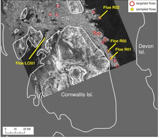
CIS specially ordered several high resolution RADARSAT-1 Standard images (25 m resolution) around Cornwallis Island in early May, about one week before the field party left for the Arctic, since the work would be conducted from PCSP in Resolute. The satellite imagery showed individual floes within a highly concentrated area of landfast multi-year ice north of Cornwallis Island (Figure 2). This band of landfast multi-year ice extended south into Pullen Strait (along the west coast of Cornwallis Island) and south into Wellington Channel (along east coast of Cornwallis Island). The presence of multi-year ice to the west, north and east of Cornwallis Island was advantageous because it allowed the field party to sample ice in different areas should there be inclement weather in one location.

Figure 2 shows the 14 multi-year floes (ranging from less than 1 km across, to 6 km across) that

were pre-selected from the 13 May Standard RADARSAT-1 image1. The targeted floes were

purposely selected to be within about 100 km of Resolute because past experience has shown that to be an acceptable distance – it minimizes time in the air (maximizes time on the ice) and facilitates the transport of personnel and equipment to the floe. Since two trips are normally required to transport personnel and the full suite of equipment to the multi-year floe, it is essential that floes be less than 100 km from base camp. The option of caching equipment along the east coast of Cornwallis Island was also examined, should it be necessary to do so.

The field work was conducted from mid-May to early June. The field party consisted of two people from National Research Council’s Canadian Hydraulics Centre (NRC-CHC) and one, or two, assistants (see Appendix A).

5.1 Sampled Floes

Four floes were sampled during the field program; three of which had been pre-selected from satellite imagery (Floes R01, R02 and R05). The fourth floe (Floe LCI01) was visited west of Cornwallis Island, in an area that had been overlooked in the satellite image because the floes were small and indistinct. Floes R01, R02 and R05 were all aggregate floes since they were comprised of sub-floes, imperceptible in the satellite image. Table 1 lists the size of the aggregate floe (estimated from satellite imagery) as well as the size of the sub-floe on which measurements were made (estimated from aerial photographs). It was extremely difficult to determine where the boundaries of one floe stopped, and another began because the ice was covered by up to one metre of snow. The rubbled perimeter of the multi-year floes was the main

(23)

feature used to estimate floe size from the aerial photographs. The estimates given in Table 1 are best guesses – aerial photographs are included in the report, so that the reader can make his or her own best guess about the size of the sampled sub-floes.

targeted floes sampled floes Floe R01 Floe R02 Floe R05 Floe LCI01 Cornwallis Isl. Devon Isl.

Figure 2 Floes pre-selected from 13 May 2008 RADARSAT Standard image (open circles). (RADARSAT-1 image courtesy of Canadian Ice Service).

Table 1 Multi-year floes sampled during 2008 field program

Floe ID date visited position (N, W) distance to floe size of aggregate floe, from satellite approx. size of sampled floe, from observations depart PCSP – return PCSP arrive floe – depart floe R01 Wellington Channel 24 May 75°17.278 93°26.014 75 km 3 x 4 km 200 m 10:00 – 18:20 10:45 – 17:45 LCI02 Pullen Strait 27 May 75°32.248 95°50.575 90 km -- 250 m 12:00 – 19:30 12:50 – 18:45 R02 Wellington Channel 30 May & 3 June 75°41.491 93°40.806 110 km 3.5 x 2.8 km 300 m 14:05 – 23:10 15:05 – 22:25 R05 Wellington Channel 5 June 75°21.891 93°26.873 82 km 1.5 x 1.7 km 200 m 9:50 – 23:40 10:20 – 22:00

(24)

Flying over Wellington Channel and Pullen Strait confirmed what was seen in the satellite imagery: multi-year floes were plentiful along the east and west coast of Cornwallis Island. The floe size, ice freeboard, hummocked surface (still evident through the snow cover) and rubbled perimeter were signs that the floes qualified as multi-year ice. It was quickly realized that finding floes on which to make detailed thickness measurements would not be a problem, but deciding which floes would be recipients of the two, 10 m long temperature chains might be. That decision had to be made before takeoff so that the proper equipment could be packed each day. Not only was it very unlikely that the field party would have the chance to visit the same floe twice, it was imperative that the amount of equipment be minimized to allow for a larger field party and to carry enough fuel to maximize the helicopter’s range. Cargo space in the 206LR helicopter was precious, and did not allow transporting unnecessary equipment. Thankfully, strapping the 2.5 m long ABS tube for housing sections of the temperature chain to the helicopter skid was permitted (Figure 3).

Figure 3 Transporting temperature chain to Floe R02. The five 2 m lengths of temperature chain were sealed in a black ABS tube and securely strapped to the helicopter skids.

5.2 2008 Field Program: Unqualified Success?

During the planning stages of the field project, it was hoped that two weeks would be sufficient to conduct detailed thickness measurements on up to 11 multi-year ice floes, and obtain additional information about the strength, temperature and salinity of the two floes on which temperature chains were installed. Due to poor weather, the field program did not proceed as planned and was, therefore, extended to three weeks. The field party arrived in Resolute on 17 May, but just barely, because poor weather nearly delayed their inbound flight from Iqaluit. And that would have put the project behind schedule by several days, at least, due to the infrequency of flights to Resolute, combined with continued weather trouble. The field party arrived in Resolute amid high winds and freezing rain. Foul weather persisted throughout the entire field program, which finally terminated on 7 June (with much hand-wringing), after

(25)

having extended the trip by almost one week. Resolute was not the only place to suffer – weather across the Arctic was extremely poor, causing significant problems at most of the remote field camps. One of the advantages of working from Resolute is that scientists can request weather reports from PCSP’s office on an hourly basis – much to the dismay of the PCSP’s office staff, to be sure!

During the three weeks spent in Resolute, the weather improved to ‘marginal’ status on just four occasions. The field party took full advantage of those four days, venturing east or west, wherever the weather was better, and spending long days on the ice to complete as many objectives as possible. While the 2008 field program certainly can’t be called an ‘unqualified success’, quite a lot was accomplished despite the frustrations met with day after day (see Appendix A).

6.0 Results from Field Study

This section discusses the four multi-year floes sampled during the field program. Ice thicknesses are discussed, along with measurements from the two temperature chains and the drift trajectories of the two instrumented floes. A close-up of the individual floes in the 13 May 2008 RADARSAT-1 image is also given because it provides an excellent view of the aggregate floe, of which the sampled floes were only a small part. Aerial photographs and on-ice photographs indicate where transects were laid; the trampled snow left an excellent record of where lines were run, as did the roughly 30 cm diameter orange circles that were sprayed on the ice (with biodegradable marking paint) to indicate where each drill hole was made.

Ice thickness was measured using the so-called ‘drill hole technique’ (Appendix B) along transects that were mapped out with flags, spaced 10 m apart. The transects included both level ice and moderately ridged or hummocked ice, to provide an accurate picture of the floe. Since the 17 m of drill auger insufficient for penetrating the full thickness of ice last year – sometimes even when the ice appeared to be in ‘level’ (Johnston, 2008-b) – this year, enough drill auger was taken to increase the drillable depth to 30 m. However, poor weather during the program limited the amount of time on the ice. As a result, it simply was not possible to spend as much time drilling the crests of hummocks or ridges as the field party would have liked. Rather, the electromagnetic (EM) induction technique, which is a surface based measurement and is therefore much faster than the drill hole technique, was used to estimate the ice thickness in areas where drilling was not possible.

The extremely deep, wet snow cover complicated (and slowed) the field program. Drudging through the snow, which was up to one meter deep in places, meant that measurements took much longer than in late summer, when walking over the floes is virtually effortless. The technique of removing the snow from a 0.5 m square surface was used initially, so that the top ice surface could be used as a reference point and the ice freeboard (distance to the waterline) could be measured. If a large enough area of snow had been removed, the freeboard could sometimes be measured by peering down the 2” drill hole to see the distance to the waterline, however often that was not possible, even after the snow cover had been removed. The uncertain success of measuring freeboard in each drill hole, combined with the time and effort required to shovel the snow, necessitated that the field party forfeit freeboard measurements.

(26)

Once that had been decided, measurements proceeded much more quickly – (1) the undisturbed snow cover was measured at each hole, (2) drill holes were made through the snow into the ice, (3) the augers were counted one-by-one as they were removed from the ice, (4) the thickness of the ice was measured to the top of the snow cover using a special purpose ice thickness tape and (4) adjustments were made later for the recorded snow depth.

6.1 Floe R01

On 24 May, after being grounded for more than one week, the weather improved enough to fly off Cornwallis Island. It was decided to visit Floe R01 because it was only about 75 km from Resolute – a nice, close run for the first-day of sampling – and the weather there looked good. By 10:00, the helicopter pilot had received a weather report from the PCSP office that showed flying to Floe R01 would be possible, after which the helicopter was loaded and the field party departed. Figure 4 shows the outbound and inbound flight paths to/from Floe R01 (75°17.278', 93°13.014'). On the outbound flight (red markers), the pilot flew across the southern part of Cornwallis Island to skirt poor weather until he reached the coast, where he turned north to parallel the coast until reaching Floe R01. The route back to Resolute was more direct (blue markers in Figure 4) because the weather had improved considerably by that time (18:20). A relatively level area of ice towards the centre of the 3.5 km diameter aggregate floe was selected for sampling (Figure 4 inset). The helicopter landed on a level area of ice, with large hummocks behind it (“H” in Figure 5–a). The upturned, rubbled edges of this sampled sub-floe suggest that it was only about 200 m across.

Three transects were mapped in level ice and rough areas of the sub-floe by placing numbered flags at 10 m intervals. A total of 35 holes were drilled along the transects. The first 40 m of Transect 1 is believed to have been outside the sub-floe proper, since the ice was only about 4 m thick (Figure 6-a). The edge of the 200 m diameter Floe R01 was crossed at a distance of 50 m, beyond which the ice was 7 to 8 m thick. Ice thicknesses along Transect 2 ranged from 5 to 15 m, with the thickest ice occurring near the floe’s rubbled perimeter at Flag 19 (Figure 6-b). Transect 3 was made on ice ranging from 5.0 to 12.3 m thick. Again, the thickest ice occurred along the floe’s upturned edge, at Flag 35 (Figure 6-c). Voids or ‘pockets’ occurred when drilling through ice at Flags 13, 25, 34 and 35 (as noted in Appendix C) which suggested the ice had deformed recently and was not well consolidated.

(27)

Floe R01

Figure 4 Flight paths taken to and from Floe R01 in Wellington Channel.

Flight path to floe shown in red; return flight path shown in blue; coast of Cornwallis Island shown in white.

(28)

H 10 7 35 19 H 1 30 11 20 21 22 23 24 26 27 28 29 25 31 12 13 14 15 16 17 18 19 32 33 34 35 36 37 38 10 9 8 7 6 5 4 3 2 Transect 1 Transect 2 Transect 3

Figure 5 Aerial views of Floe R01 (a) photo showing extent of 200 m diameter floe and (b) transects made on floe. “H” shows where helicopter landed. The thickest ice occurred at Flags

35 and 19, along the floe’s rubbled perimeter.

(a)

(29)

-16 -12 -8 -4 0 4 0 20 40 60 80 100 120 distance (m) th ic kn e ss ( m )

Transect 1, h_i drill hole Transect 1, h_i+h_s, drill hole

Flag 1 -20 -16 -12 -8 -4 0 4 -100 -80 -60 -40 -20 0 20 40 60 80 distance (m) th ic kn e ss ( m )

Transect 2, h_i drill hole Transect 2, h_i+h_s drill hole

Flag 19 -16 -12 -8 -4 0 4 -100 -80 -60 -40 -20 0 20 distance (m) th ic kn e ss ( m )

Flag 38

Figure 6 Drill hole thicknesses for Floe R01.

Drill hole thicknesses given for ice thickness (h_i) and ice plus snow thickness (h_i+h_s). Drill hole data are tabulated in Appendix C.

(30)

Figure 7 On-ice photos of Floe R01 (a) beginning of Transect 1, (b) level ice at interior of floe and (c) view from rough ice near flag 26.

(a)

(b)

(31)

6.2 Floe LCI01

Poor weather on the morning of 27 May prevented flying to Wellington Channel (in the east), Pullen Strait (in the west) and to the northern end of Cornwallis Island. By noon, the weather had improved enough in the west to allow the field party of four to make an attempt for Pullen Strait, and hope the weather would continue to improve if indeed they made it. The coordinates of a multi-year floe in Pullen Strait (75°31.50N, 95°52.84W) and a multi-year floe in Templeton Bay (75°28.70N, 96°20.66W) were quickly worked out and given to the pilot. If the field party could not reach Pullen Strait, the ice in Templeton Bay could be sampled instead. The ice in Templeton Bay was attractive should there be marginal weather because huts at the Old Polaris mine site were nearby should temporary refuge be needed.

The flight path en route to Pullen Strait shows that the field party flew right over the coordinates of the 1 km diameter floe that had been given to the pilot (floe 1, Figure 8 inset, 75°31.50N, 95°52.84W). Evidently, he felt the floe was too rough to comfortably land on – clearly, he preferred landing on very smooth ice. Minutes after the targeted floe had been passed, another prospective floe came into view, this one about 600 m across (floe 2, Figure 8 inset). The pilot then landed in an area of smooth first-year ice adjacent to the requested area (75°32.248, 95°50.575, as shown by the “H” in Figure 9-a). The landing site was, in fact, several kilometers northeast of the 1 km floe that had been targeted originally.

Once the field party was on the ice, eyes turned from the 600 m diameter ‘prospective floe’ that had been seen from the air, to a different floe that contained a sizeable hummock, about 200 m away. It was decided that measurements would focus on the area around this 3 to 4 m high hummock (Floe LCI01). The kidney-shaped Floe LCI01 was nestled between two much larger floes which made it difficult to identify in the satellite image. Thankfully, superimposing the circular flight path that was made around the perimeter of the floe was the only way of identifying Floe LCI01 in the satellite image (Figure 8 inset). Aerial photographs suggest that Floe LCI01 was about only about 250 m long and less than 100 m wide (Figure 9).

Rather than transport all the gear to the hummock and begin there, it was decided to begin the thickness measurements in the smooth ice and approach the hummock gradually. The first hole (hole 0) was drilled next to the helicopter, where the ice was only about 2 m thick, about 30 m from where Transect 1 began (Flag 1). The ice at Flag 1 was 1.93 m thick but much thicker ice was encountered 10 m away (8.65 m, Flag 2) and beyond, indicating that the rubbled perimeter of the floe ‘proper’ had been crossed.

(32)

Floe LCI01

floe 1 floe 2

Figure 8 Flight paths taken to and from Pullen Strait, where Floe LCI01 was sampled. Flight path to floe shown in red; flight path from floe shown in blue. Floe LCI01 is difficult to

see in this Standard image, due to its small size (about 250 m long).

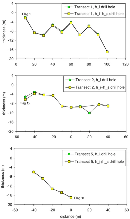
A total of 44 flags were mapped out along seven transects on Floe LCI01, as shown in Figure 9-b. Transect 1, the main line, extended from the helicopter to the crest of the 3 to 4 m high multi-year hummock. Four transects ran perpendicular to Transect 1. Transect 6 extended along the crest of the hummock and Transect 7 was made on the far side of the hummock, on a different multi-year floe. Figure 11 shows on-ice photographs along several of the transects. Drill hole measurements were made at only 23 of the 44 flags. Since arriving on the floe in the early afternoon limited the amount of time that could be spent on the ice, it was decided not to drill the crest of the hummock.

Figure 10 shows the thicknesses measured along the six transects on Floe LCI01 (excluding Transect 3, where measurements were not made). The thickest ice was drilled at Flag 10 (16.9 m thick), which was about 10 m away from the crest of the hummock where the ice would have certainly been even thicker had it been drilled. A ‘pocket’ or void in the ice at Flag 10 was encountered at a depth of about 10.4 m (as noted in Appendix C). Other pockets may have been present also, but were missed because concentration was devoted to maintaining control of the up to 19 m of drill auger in the hole. Since the ice at Flag 10 was not as ‘solid’ as ice in other holes on the floe, drilling was difficult – the drill bit did not cut through the ice as well as it should.

(33)

Thankfully, the weather in Pullen Strait held out long enough for the field party to work on Floe LCI01 for almost 8 hours. The field party departed the floe at 18:45. During the return trip to Resolute, a detour was taken to Templeton Bay (blue markers, Figure 8) to see whether one of the floes there was suitable for sampling, should the weather again dictate a change in plans. As it turned out, the floe in Templeton Bay, which looked worthy of a visit in the satellite image, was not much of a floe at all – with little freeboard and few hummocks. The field party continued on to Resolute, returning at 19:30.

39 10 3 19 B3 H 10 9 8 5 4 3 6 20 21 22 23 13 14 15 12 11 7 16 17 39 38 37 36 35 34 24 18 19 25 26 27 28 29 30 31 32 33 B1 B2 B3 B4 B5 Transect 1 Transect 2 Transect 3 Transect 4 Transect 5 Transect 6 Transect 7

Figure 9 Aerial views of Floe LCI01 (a) Flag 10 shows where the thickest ice was measured on the floe (16.9 m thick) and (b) seven transects that were mapped on floe.

(a)

(34)

-20 -16 -12 -8 -4 0 4 0 20 40 60 80 100 120 distance (m) th ickn e s s ( m )

Flag 1 -20 -16 -12 -8 -4 0 4 -60 -40 -20 0 20 40 60 distance (m) thi c k nes s ( m )

Flag 15 -20 -16 -12 -8 -4 0 4 -60 -40 -20 0 20 40 60 distance (m) th ickn e ss ( m )

Flag 10

Figure 10 Drill hole thicknesses for Floe LCI01 (transects 1, 2 and 5 – the three transects along which drill holes were made).

(35)

Figure 11 On-ice photos of Floe LCI01 (a) Transect 1 beginning where helicopter landed in level first-year ice, (b) end of Transect 1 leading up to hummock and (c) adjacent floe, on other side of hummock.

(a)

(b)

(36)

6.3 Floe R02

By 30 May the reality of not fulfilling all the project’s objectives was beginning to dawn on the field party – two weeks had passed and only two floes had been sampled; neither temperature chain had been deployed. The project was reaching a critical stage. On the morning of 30 May, PCSP indicated that the weather did not look good, but “the field party was welcome to venture out to see how far it could get”. Realizing there were only a few days left to the program, at most another week if the trip was extended, the field party decided to give Wellington Channel a try. The helicopter was packed with one of the temperature chains and the field party departed Resolute at 09:55. Ten minutes after takeoff, they met a wall of fog and were forced to turn back. The helicopter was back on the ground in Resolute at 10:20. Conditions to the east of Resolute were the same.

In the afternoon, another attempt was made to reach Wellington Channel. The field party departed Resolute at 14:05. This time the weather cooperated. The targeted floe was located at the north end of Wellington Channel, which satellite imagery suggested was about 3.5 km by 2.8 km across (Figure 12). The field party flew over Lake Elanor while en route to the floe, to explore the option of using one of the cabins at the Lake as a remote base camp (see Appendix A). Once a reconnaissance of Lake Elanor had been conducted, the field party proceeded to the pre-selected floe.

The aggregate multi-year floe was comprised of many smaller floes, with ridges in between. The sampling area selected as Floe R02 was about 500 m from the edge of the aggregate floe (Figure 12 inset). At 15:05, the helicopter pilot landed on a suitably level area on Floe R02. The satellite image shows the floe that was sampled, northeast of which another similarly shaped floe was located, with a bright linear region of rubbled ice separating the two floes (Figure 13). Evidently, this floe was a very popular spot for polar bears – since the ice was covered with bear tracks. The ‘draw’ for the bears was likely the rubbled first-year ice along the frozen lead that had formed earlier in the season, which appears to have happened when the north end of the aggregate floe pulled away from the main floe (Figure 13). The frozen lead was about 100 m wide.

The first order of business was to find a suitable location for the temperature chain, the objective being to install the 10 m long temperature chain in ice of equal thickness to make use of all the ice sensors. The first drill hole was made on a small knoll (Flag 1, Figure 14), where the ice was 7.6 m thick – not quite thick enough for the temperature chain. The second drill hole was made on a larger knoll, about 60 cm high, where the ice was 10.20 m thick (Flag 25.5, Figure 14), a suitable thickness for the temperature chain. As two of the field party began installing the temperature chain, the third person laid out 39 flags along six transects.

The aerial photograph in Figure 14 shows where the helicopter landed (as denoted by a circled “H”, 75°41.491N, 93°40.806W) and the transects that were made on Floe R02. Only a 14 holes were drilled on Floe R02 – the best the field party of three could do given the late start and the work involved in installing the temperature chain (Appendix B). Installing the temperature chain took several hours, sometimes requiring the help of all three members of the field party. Wiring the sensors to the logger was time consuming (taking one hour to complete) but since it only required one person, the other two people made most of the drill hole measurements during that time. Once the temperature chain had been fully installed, two of the field party conducted EM measurements as the third person measured snow depths.

(37)

Floe R02

Figure 12 Flight paths taken to and from Floe R02, at the north end of Wellington Channel. Flight path to floe shown in red; flight path from floe shown in blue.

Figure 16 and Figure 17 show the surface conditions on Floe R02. Transect 1 started near the helicopter (Flag 1, 7.6 m thick) and ended in ridged area of ice on the other side of the floe (Flag 10, 14.1 m thick). Most of the other drill holes were made along Transects 5 and 6, where the ice was from 6.34 to 10.42 m thick. The photographs in Figure 17 show (a) the knoll where the temperature chain was installed along Transect 1 and (b) the ridge crest along which EM measurements were made (Transect 2). Figure 15 shows the profiles from the 14 drill holes, most of which were made along Transects 5 and 6 (Appendix C). EM measurements were made at all 39 flags.

(38)

temperature chain temperature

chain

refrozen lead

instrumented floe adjacent floe

linear ridge separating two floes

Figure 13 Aerial photographs showing surface features on Floe R02.

(a) floe on which the temperature chain was installed, (b) floe adjacent to the sampled floe, beyond which smooth first-year ice extended and (c) re-frozen lead that formed at the north end

of the floe.

(a) (b)

(39)

H 21 1 25 26 27 28 29 30 31 32 3335 3637 3839 34 24 22 23 2 3 4 5 6 7 8 9 10 11 12 13 14 15 16 17 18 20 temperature chain Transect 1 Transect 2 Transect 3 Transect 4 Transect 5 Transect 6

Figure 14 Aerial view of Floe R02 showing flag positions and helicopter landing site (“H”)

-20 -16 -12 -8 -4 0 4 0 20 40 60 80 100 120 140 distance (m) thi c k nes s ( m )

Flag 1 Flag 10 -20 -16 -12 -8 -4 0 4 -140 -120 -100 -80 -60 -40 -20 0 20 distance (m) thi c k nes s ( m )

Flag 34

(40)

Figure 16 On-ice photos of Floe R02 showing (a) Transect 1 beginning near the helicopter and (b) Flag 10 where the ice was 14.1 m thick (circled flag).

(a)

(41)

Figure 17 On-ice photos of Floe R02 (a) where temperature chain was installed on Transect 5 and (b) conducting EM measurements along ridge crest at Transect 2

(a)

(42)

6.3.1 Installation of Temperature Chain on Floe R02

The 60 cm high knoll between Flags 25 and 26 was selected for installing the temperature chain because that is where the ice was 10.20 m thick (75°41.46N, 93°40.82W). The reader is referred to Appendix B for a complete description of the installation, but some of the main points will be mentioned here. Once the full thickness of ice had been drilled, the appropriate section of 2” PVC pipe was lowered into the hole (Figure 18-a), making sure to keep it moving so that it would not freeze in place before the entire assembly had been installed. Once the five sections of the temperature chain had been lowered into the hole, it was positioned level with the ice surface and fit snugly in place. Two L-brackets were mounted flush with the top ice surface to indicate where the original ice surface had been, so that a measurement of the amount of surface melt could be taken when the floe was re-visited later in the fall. The deepest ice sensor (10 m depth) was located about 0.20 m above the bottom ice.

Once the temperature chain was in place, its five bundles of lead wires were fished through a flexible metal conduit that ran from the top ice to the data acquisition system. After more than 90 wires had been connected to the data logger, a check was made to verify that all sensors functioned properly. The plywood housing for the data acquisition system and battery was assembled and then fasted to four PVC legs that were frozen two metres into the ice.

Installation was complete by 20:45, as shown in Figure 18-b. It should be noted that a considerable amount of thought went into designing a system that, while it was not necessarily bear-proof, would somewhat discourage curious bears from damaging the system. As it turns out, that was wise because Floe R02 was a favorite site for bears, given the abundance of animal tracks.

6.3.1.1 Second Trip to Floe R02

The day after the temperature chain had been installed on Floe R02, data were downloaded remotely from Ottawa and sent to the author in the field. It was soon realized that one of the sensors had been wired improperly (960 cm) and several others had malfunctioned several hours after they were installed. A few malfunctioning sensors would not normally be cause for re-visiting a floe, but the CALIB (Compact Air Launch Ice Beacon) that had been installed on Floe R02 was not working either2 and it needed to be recovered. Thankfully, a second GPS system had been incorporated into the data acquisition system for the temperature chain, to provide independent measurements of Floe R02’s position, and provide redundancy.

On June 3, a Twin Otter came available for transporting the field party and their gear to Lake Elanor (in hopes of establishing a remote base camp). Camping supplies were quickly packed, and the plane was loaded for departure. After touching down at Lake Elanor, the pilots were asked if it would be possible to make a short detour to Floe R02 so that the malfunctioning temperature sensors could be corrected and the CALIB retrieved. A radio check was made to PCSP to see if the detour was permissible: it was.

2_{In the past, the Canadian Ice Service has generously provided CALIBs to document the drift of multi-year floes.}

CALIBs have proven reliable, although they are expensive and they sometimes malfunction. In this case, there was no way of knowing about the problem when the beacon was deployed. The CALIB was recovered on June 3 and shipped back for investigation, where it was concluded that a wire had come loose during shipping.

(43)

Because the surface of Floe R02 was too rough for the Twin Otter to land, the 100 m wide frozen lead of first-year ice was used as a landing strip instead. Since the lead was only about 500 m from the temperature chain, the field party could climb to the top of a nearby hummock to spot the bright orange box. They then walked the short distance through rubbled ice to the box. As soon as they arrived, the problem with the temperature chain became clear: a bear had gnawed on the flexible metal conduit, shaking three of the sensors loose and exposing the bundled lead wires coming out of the top of the PVC pipe – all this had happened, just hours after the temperature chain had been installed. The malfunctioning sensors were reattached to the data logger, the exposed leads were again covered and the CALIB beacon was recovered.

Figure 18 Temperature chain ‘A’ on Floe R02 (a) installing temperature chain between flags 25 and 26 on Transect 5 and (b) completed installation with elevated orange box housing the data

acquisition system, GPS and Iridium phone communications.

(a)

(44)

6.3.2 Documented Changes in Floe R02

The temperature chain on Floe R02 transmitted data from 30 May to 30 July, providing a record of daily ice temperatures every 15 minutes. Figure 19 shows weekly changes in the ice temperature profile using measurements acquired every Sunday at 06:00. Temperatures are also included for 30 May (21:15), about one hour after the chain was installed, to provide an indication of the ice conditions shortly after seawater flooded the drill hole and began to freeze.

Top surface of ice: The greatest increase in temperature occurred at depths 2.0, 2.4 and 2.8 m

(increases of 9.8°C, 9.9°C and 9.6°C respectively). Had the temperature chain been installed earlier in the season, it is expected that the top ice surface would have experienced the greatest increase in temperature, since that is where the ice would have been coldest. Although the most significant changes in temperature occurred at the 2 to 3 m depth, the ice to a depth of about 8 m showed evidence of warming. Meltwater percolation may explain temperature changes below the first several metres, since solar radiation has a limited penetration depth.

Bottom surface of ice: In comparison to the dramatic changes in temperature that occurred

towards the top ice surface, the ice below a depth of about 8 m warmed to a lesser extent. From 29 June to 6 July temperatures at the 10 m depth warmed from to -1.2°C from -1.8°C (the freezing point of seawater). Increases in temperature at this depth likely resulted from warming of the seawater around the floe. During the last three weeks of July, the ice at the 9.2, 9.6 and 10.0 m depths cooled by several tenths of a degree per week. Cooling in the bottom layer of ice at that time may have been caused as the floe encountered colder water during its northward drift (Figure 20). -12 -10 -8 -6 -4 -2 0 2 -14 -12 -10 -8 -6 -4 -2 0 2 4 6 8 10 Tem perature (°C) De p th ( m ) 30 May - install Jun 1 Jun 8 Jun 15 Jun 22 Jun 30 Jul 6 Jul 13 Jul 20 Jul 27 Jul 30 Floe R02

ice bottom on 30 May

NOTES:

• communication with the ice sensors was permanently disrupted on 30 July.

• temperatures at a height of “+1.0 m” were actually measured inside the data logger box not on the temperature chain itself.

• the sensor at 0.0 m was level with the top ice surface when the chain was installed.

(45)

6.3.3 Tracking the Drift of Floe R02

The position of Floe R02 was monitored from 31 May to 20 September using the GPS that had been incorporated into the temperature chain. The bear attack that occurred at the end of July severed the temperature sensors from their data acquisition system, terminating the entire suite of ice temperature measurements, however (thankfully) the GPS system on Floe R02 continued to function until mid-September.

GPS data were only logged four times per day, to conserve battery power (10:00, 10:15, 15:00 and 15:15). The GPS data were downloaded remotely from Ottawa between 07:30 to 08:00 (i.e. the same “window” as the data from the floe’s temperature chain). Figure 20 shows the drift of Floe R02 from 31 May to 20 September. Since communication with the floe was sometimes intermittent, open circles have been used in the map to provide some indication of the floe’s position when data are not available.

Floe R02 traveled more than 1000 km. The floe first started moving on 17 July, as the landfast ice around it broke-up, traveling north until 13 August and then changing direction to drift south past Little Cornwallis Island, towards Parry Channel. By 25 August, the floe was migrating south along the coast of Bathurst Island. It then turned north into Austin Channel, after which it drifted south across Parry Channel, and into M’Clintock Channel. Communication with the floe was lost on 20 September which, unfortunately, occurred just prior to the CCGS Louis S.

St-Laurent passing through the area. Therefore all attempts to re-visit the floe with the ship’s

assistance were aborted.

Although the communication link to Floe R02 was tried every day from 7 September to late November, the only attempt that met with (partial) success occurred on 20 September. On that day, the computer in Ottawa connected to the floe’s data acquisition system long enough to make a screen capture of the data logger’s status window (indicating the date, time, GPS coordinates and battery voltage). What happened to Floe R02 after 20 September? The failed communication was not due to a lack of battery power because the battery voltage on 20 September was 11.8 V, well above the required minimum voltage of 10.5 V. Other reasons for why the system failed include (a) the data acquisition system taking on water, although it was elevated to prevent this, (b) the floe may have collided with some feature that destroyed the instrumentation, (c) the portion of the floe in which the temperature chain was installed could have severed from the floe since it was only about 500 m from the floe edge (Figure 12 inset). Even more likely, however, is that (d) the difficulty communicating with the floe resulted from snow/ice attenuating the signal from the antenna or (e) subzero temperatures causing the phone to malfunction, even though the phones are rated to -20°C.

(46)

31 May 23 Jul 1 Aug 13 Aug 17 Aug 25 Aug 2 Sep 7 Sep 20 Sep Parry Channel M’Clintock Channel Wellington Channel Austin Channel Resolute

Figure 20 Migration of Floe R02.

Drift shown from 31 May 2008 (the day after the floe was instrumented) to 20 September 2008 (when all communication with the floe was lost). Open circles show floe’s approximate position

where data are missing.

6.4 Floe R05

On 5 June the helicopter departed Resolute for Pond Inlet, where it was needed to support a different field study, leaving the Twin Otter as the only mode of accessing one last floe in Wellington Channel. Never having accessed multi-year ice by Twin Otter, but knowing that others had3, the field party decided to try it – especially if it meant sampling one more floe. On 5 June, the weather improved enough for the field party of three to access a floe in Wellington Channel by Twin Otter. The intention was to remain on the floe until late evening, when the plane would return. All agreed that the field party must take provisions and camping gear in case the weather closed in and the plane did not make it back that evening. The plan would also require transporting one of the snowmobiles, the komatik and camping gear that had been left at Lake Elanor on 3 June (in preparation for establishing a remote base camp) to the targeted floe in Wellington Channel. The Twin Otter would fly to the floe, leave two of the three people in the field party and their equipment, fly to Lake Elanor and then return to the floe with the additional supplies.

3_{Some people use Twin Otter aircraft to access multi-year ice, rather than helicopters, but usually it is because Twin}