R esear ch Ar ticle Building Ther mal , Ligh ting , and A coustics M o d eling E-mail: david.daum@epfl.ch
Assessing the saving potential of blind controller via multi-objective
optimization
David Daum( ), Nicolas Morel
Solar Energy and Building Physics Laboratory (LESO), Swiss Federal Institute of Technology Lausanne (EPFL), 1015 Lausanne, Switzerland
Abstract
This paper presents the results of computational experiments where multi-objective algorithms were used to tune a controller for blind movements in a residential building and a room of the LESO (Solar Energy and Building Physics Laboratory) experimental building. The blind controller, which is based on fuzzy logic, was optimized not only in terms of energy consumption but also in terms of thermal comfort. The goal is to show saving potential for intelligent blind controller in a real world example rather than in tailored idealized test rooms. Therefore, a state of the art simulation program with a multi-objective evolutionary algorithm was combined. It was found that with elementary control systems, like schedules for the lighting in a building, almost 40% of the energy could be saved. With the help of more advanced controllers this can be further increased. Also discussed in this paper are the results and the feasibility of implementing such a controller.
Keywords
multi-objective optimization, simulation,
smart blind controller, fuzzy logic, energy efficiency Article History Received: 26 May 2009 Revised: 19 August 2009 Accepted: 20 August 2009 © Tsinghua University Press and Springer-Verlag 2009
1 Introduction
Energy efficiency for buildings has always been a topic of interest, but with increasing energy costs the attention given to this field is growing. The main proportion of energy in the housing sector is used for space heating and cooling. Therefore, a good control of the blinds is important as they significantly influence the thermal profile of a building via heat gains. This means that in the winter period the heat is kept inside and in the summer the blinds help keep the heat outside. As the control of these and other complex systems in a building are not trivial, automatic controllers for technical equipment are used more and more. On the other hand, the accuracy of design tools and simulation software has improved in recent years, which allows proper analysis of the performance of such a controller. For assessing the saving potential we use one room of the LESO (Solar Energy and Building Physics Laboratory) experimental building that we modeled with the IDA ICE (IDA Indoor Climate and Energy) building simulation software. This allows us to test different types of blind controllers in a fast
and exact manner. To point out the influences of blinds we compared the average transmitted power with closed and opened blinds. It was then simulated at the south oriented LESO room average power, for a given week, amounts to 529 W with opened blinds, and only to 49 W with closed blinds.
For the occupants, the aspect of comfort is equally important. In fact a study showed that in the USA the direct and indirect costs due to suboptimal working conditions are estimated to 26 billion dollars per year (Leigh et al. 1997). In literature there is already a big variety on different principles for controllers including PID (proportional integral derivative), fuzzy and artificial neural networks being proposed. Particularly in the domain of HVAC (heating, ventilating, and air conditioning) control fuzzy- logic appear to be one of the main choices for developers (Dounis and Manolakis 2001; Calvino et al. 2004; Jian and Cai 2000). Fuzzy-logic was also applied successfully in the field of blind controllers. For example, in (Lah et al. 2006) a fuzzy-logic system for managing a roller blind in respect to the light inside the building has been developed. In (Guillemin and Molteni 2002) an energy efficient controller
for shading devices was proposed which is based on fuzzy logic and self-adapting to the user’s wishes. Kolokotsa (2003) analyzed the performances of different fuzzy controllers for the PMV (predicted mean vote) and CO2concentration. All fuzzy controllers were able to satisfy well their task and showed only slight differences in performances. The successful application of fuzzy-logic in connection with building controllers can be attributed to the fact that the approximate reasoning logic of the human brain, which is the decision maker in the real world, is well reflected by fuzzy-logic theory. Our system for blind automation, which we aim to optimize is also based on a fuzzy system and will be explained later in detail.
In most of the publications it is shown that their proposed controller in terms of energy consumption is superior to an on-off controlled counterpart (Galasiu et al. 2004; Kolokotsa 2003; Kolokotsa et al. 2001). Unfortunately the complete saving potential has as far as we know not been evaluated. Our goals are to optimize the energy efficiency of our controller and on the other hand to introduce as a second objective a measurement for thermal comfort. This gives us the possibility to identify the complete saving potential and furthermore establish a trade-off between user-comfort and energy-efficiency. For a more realistic simulation we introduce stochastic models to handle occupancy, internal loads and artificial lighting which influences the energy consumption directly.
2 Experimental setting
In this section we consider two different experimental settings, the first consists of the Room 002 from the LESO experimental building in Lausanne and the second is a flat located in a residential apartment building in Lucerne.
2.1 LESO experimental building
The setup of the first experiment can be seen in Fig. 1. It was modelled with IDA ICE according to its real dimensions. With regards to the window we did not model the daylighting system of LESO (Altherr and Gay 2002) with an anidolic and a normal window, instead we used just one window with the combined size of these two windows. The model room has no exterior walls except for a south oriented wall with a window. We make the hypothesis, that from the north and south there are no other buildings that, importantly, could block the sunlight. It is located in Lausanne, Switzerland at a latitude of 46.53°longitude of 6.67°and altitude of 380 m. For the simulation the 2007 weather data from Lucerne is used as the second building
Fig. 1 Floor plan of the LESObuilding
is located in Lucerne and we wanted to make the results comparable.
Blind External textile blind, total shading coefficient:
0.14, short wave shading coefficient 0.2, no influence on the U-value
Room Floor area of a room: 15.7 m2, room height: 2.8 m
External wall Facade wall (to south): 5.4 m2, light wall
(1 cm plaster panel +12 cm thermal insulation + 1 cm wood)
Internal wall Light partition wall (1 cm plaster panel +
4 cm thermal insulation +1 cm plaster panel)
Floor 15.7 m2 (1 cm rubber coating+6 cm screed +
6 cm thermal insulation +25 cm concrete slab)
Window 3.8 m2 net area (double-glazing with IR coating,
U-value: 1.4 W/(m2·K))
2.1.1 Heating system
The room is equipped with one electric radiator that is positioned below the window and has a setpoint of 21℃. The LESO building is not equipped with an air conditioning unit but we introduced one in the simulation to measure the unpleasant heat increases in terms of energy.
2.1.2 Occupation
As each human being emits heat and pollutants, her/his presence directly changes the indoor environment. In addition to that, the interaction with electrical appliances as well as the use of artificial lighting increases the internal heat accumulation and the consumption of electricity. In an office building it is mostly the computer and, for example, the coffee machine that are responsible, while in residential buildings the focus will be on the dishwasher and dryer as the biggest consumers. Additionally occupants also interact with the building to enhance their thermal and visual comfort by using the windows, doors and blinds. These interactions will in turn affect the energy consumption for the buildings HVAC unit. We use the stochastic models developed at LESO by Jessen Page (Page et al. 2008) as they include the latest development in this field of study and
are adaptable to our requirements.
In our simulation the occupant has direct influence on: Productions of internal metabolic heat gains and pollutants Use of appliances (additional heat gains)
Use of artificial lighting (additional heat gains)
The occupancy density in our office is 10 m2 net area per person with a metabolic rate of 1.2 met and heat emissions of 70 W/person. The probabilities of occupancy are given in Table 1.
2.1.3 Electric equipment
There are two kinds of appliances: the ones that operate independently of the user’s presence (for instance a refrigerator), and those that are directly driven by the occupancy (for instance, a computer or a TV set). In the latter category, some appliances are only driven by the occupancy (for instance, a computer in an office room), and some are additionally following a profile of use (for instance, a TV set, which is biased towards the evening, or a cooker, which is biased towards the one or two hours time intervals before meals). The stochastic model, which we use to simulate the load of the appliances, was developed at LESO by Jessen Page. For further information we refer to (Page et al. 2008).
2.1.4 Artificial lighting
How artificial lighting is used depends mostly on the occupant and whether there are automated schedules already installed in the building. To simulate the attitude towards the usage of artificial lighting we implemented the Lightswitch 2002 algorithm (Reinhart 2004) which simulates the switching behavior of occupants. This gives us a realistic feeling of the periods where artificial lighting is most probably used and can adapt accordingly. The installed nominal power in the LESO room is 4.5 W/m2 with an efficiency of 55.2 lm/W.
2.2 Residential apartment building
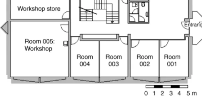
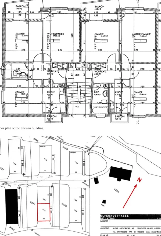
The second experiment setup consists of a flat located in a residential apartment building (see Figs. 2 and 3). The whole building was modeled with IDA ICE according to its real
dimensions but only one flat was equipped with the blind controller for optimization (see listing). The building is surrounded by other buildings which have been integrated in the computational model (see Fig. 4). It is located in Lucerne, Switzerland, at a latitude of 47.02°, longitude of 8.19°and altitude of 477 m. For simulation, the data is from the SIA climatic data collection for the station Lucerne, which is located at a latitude of 47.02°, longitude of 8.18° and altitude of 456 m.
Rolling shutters External blind, total shading coefficient:
0.17, short wave shading coefficient: 0.17, U-value coefficient: 0.9 (that means that with lowered blinds, the U-value of the window is multiplied with 0.9)
Apartment Floor area of flat: 65.4 m2, room height:
2.3 m
External wall Facade wall: 5.4 m2, light wall (1 cm plaster
panel +30 cm brick masonry +1.5 cm mineral render), U-value: 1.19 W/(m2·K)
Internal wall Light partition wall (1 cm plaster panel
+4 cm thermal insulation +1 cm plaster panel)
Floor 65.4 m2 (2 cm wood parquet +8 cm cast cement
+30 cm reinforced concrete)
Window 10.95 m2 net area (U-value: 2.9 W/(m2·K)), living
room southwest: 1.95 m×1.32 m, bedrooms northeast and southeast: 1.25 m×1.32 m, bathrooms northeast and southeast: 1.0 m×1.0 m, balcony door kitchen northeast: 1.13 m×2.23 m, balcony door bedroom southwest: 0.70 m
×2.23 m
2.2.1 Heating system
The building is equipped with three radiators per apartment which are positioned below the windows. Thermostatic valves with a set point of 21℃ control them. An oil boiler with 0.8 annual efficiency works the heat generation for heating and domestic hot water.
2.2.2 Occupation
For modelling the inhabitants the same stochastic model employed in the first setting is used (see Section 2.1.2). The occupancy density in our flat is 32 m2 net area per person with a metabolic rate of 1.2 met and heat emissions of
Table 1 Probabilities for occupancy on weekdays and weekend for the LESO office building
Time 1:00 2:00 3:00 4:00 5:00 6:00 7:00 8:00 9:00 10:00 11:00 12:00 Weekday 0.00 0.00 0.00 0.00 0.00 0.00 0.05 0.10 0.70 0.70 0.70 0.70 Weekend 0.00 0.00 0.00 0.00 0.00 0.00 0.01 0.01 0.05 0.05 0.05 0.05 Time 13:00 14:00 15:00 16:00 17:00 18:00 19:00 20:00 21:00 22:00 23:00 24:00 Weekday 0.20 0.60 0.70 0.70 0.70 0.70 0.70 0.10 0.01 0.01 0.01 0.00 Weekend 0.01 0.01 0.01 0.00 0.00 0.00 0.00 0.00 0.00 0.00 0.00 0.00
Fig. 2 Floor plan of the Elfenaubuilding
Fig. 4 3D view of the building in the IDA ICE software
70 W/person. The probabilities of occupancy are given in Table 2.
2.2.3 Electric equipment
Again the same stochastic model used in the first case is again applied and the description can be found in Section 2.1.3.
2.2.4 Artificial lighting
The installed nominal power is 9.4 W/m2 with an efficiency of 65 lm/W. An explanation of how the artificial light is switched on and off can be found in Section 2.1.4.
3 Framework of the optimizer
Optimizing a system with many parameters where the relation between them may not simply be understood proved that conventional optimization techniques are not always the best choice. As the results for the fitness function in this case are provided by an external simulation program that acts like a black box, genetic algorithms (GA) seemed well suited. Given that we will deal with two objectives, the energy consumption and the thermal comfort, a multi- objective evolutionary algorithms (MOEA) will be used for the optimization of the blind controller.
3.1 Multi-objective optimization
Like in many real world problems we deal with two objectives
that contradict each other and therefore we cannot identify “one” optimal solution. Hence for the decision making it is important to know the trade-off between the solutions by computing the pareto-optimal frontier. To best handle that task a variety of genetic strategies have been proposed in recent years (for an overview see for instance (Deb 2000; Coello Coello et al. 2002)). Let us consider a typical multi- objective optimization problem:
( ) 1 ( ) Minimize ( ( ),..., ( )), ( ) Subject to ( ) 0, L m k U f f g x ≤ ≤ ≥ x x x X x X 1,2,..., k= K (1)
here fm are the objective functions, gk the constraints and
( ) ( ) , L U
X X the bounds for the parameter vector x. For finding the reliable frontier NSGA-Ⅱ (non-dominated sorting genetic algorithm) has been applied. The used parameters of the algorithm are given in Section 5.
3.2 Layout of the optimization
To perform the optimization we combined two independent programs: the NSGA-II (Deb et al. 2002) optimization algorithm and the IDA ICE 3.0 (IDA Indoor Climate and Energy) program (Sahlin et al. 2004). IDA ICE is a dynamic building simulation program that makes simultaneous performance assessments of all parts of the building: energy consumption, light, shape, envelop glazing, HVAC, systems, controls, indoor air quality, etc. The accuracy of IDA ICE has been assessed by the IEA solar heating and cooling program, Task 22, subtask C (Achermann and Zweifel 2003). Furthermore, IDA ICE has been chosen as one of the major 20 building energy simulation programs (Crawley et al. 2005). The IDA ICE simulation tool is iteratively called by the NSGA-II via batch mode whenever there is an evaluation of the fitness function needed. The results from the optimization are given back to NSGA-II, which is evaluating the fitness functions and changing the design variables according to its crossover and mutation operators. With the new design parameters the IDA ICE is called again until termination criteria is fulfilled. The operation diagram is given in Fig. 5.
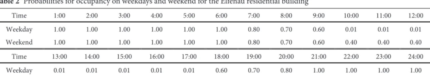
Table 2 Probabilities for occupancy on weekdays and weekend for the Elfenau residential building
Time 1:00 2:00 3:00 4:00 5:00 6:00 7:00 8:00 9:00 10:00 11:00 12:00 Weekday 1.00 1.00 1.00 1.00 1.00 1.00 0.80 0.70 0.60 0.01 0.01 0.01 Weekend 1.00 1.00 1.00 1.00 1.00 1.00 0.80 0.70 0.60 0.40 0.40 0.40 Time 13:00 14:00 15:00 16:00 17:00 18:00 19:00 20:00 21:00 22:00 23:00 24:00 Weekday 0.01 0.01 0.01 0.01 0.01 0.60 0.70 0.80 1.00 1.00 1.00 1.00 Weekend 0.40 0.40 0.40 0.40 0.40 0.60 0.70 0.80 1.00 1.00 1.00 1.00
Fig. 5 Operation diagram of NSGA-II and IDA ICE
To fit the IDA ICE software to the specific needs of the user it is possible to write your own components and connect them to the simulation process. They are written in the “neutral model format” (NMF) from which it is also possible to call functions written in C. For that reason our blind controller with the fuzzy-logic system is written in C embedded in a NMF module, which is connected to the window model of IDA ICE. To verify the functionality the fuzzy-logic controller was also implemented with MATLAB and compared to the results obtained by our algorithm.
According to (Herrera et al. 1995) there are two main ways of adapting fuzzy systems with GA’s: first by generating rule sets and second by changing parameters in the membership functions. As the fuzzy rules are based on a real world tested controller (Guillemin 2003) we apply the second possibility. Generally the parameters of the mem- bership functions are used for modification. But because we use a Sugeno (1985) type fuzzy inference and the outputs (xi) are crisply defined, only these are considered for the
adaption. Within these controller attention is mostly given to thermal aspects, and the rules are as follows:
(1) If Season is winter and Iglob is night then α=x1 (2) If Season is winter and Iglob is high then α=x2 (3) If Season is winter and Iglob is mid then α=x3 (4) If Season is winter and Iglob is low then α=x4 (5) If Season is summer and Iglob is night then α=x5 (6) If Season is summer and Iglob is high then α=x6 (7) If Season is summer and Iglob is mid then α=x7 (8) If Season is summer and Iglob is low then α=x8
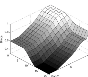
Iglob corresponds to the global vertical illuminance (lx) on the window plane and Season corresponds to the current outside temperature (℃). The output values α correlate directly with the blind setting, where α =0 means the blind is closed and α =1 stands for blind is open. The membership functions are shown in Figs. 6 and 7, and the corresponding response surface is shown in Fig. 8.
Fig. 6 Membership function of Iglob
Fig. 7 Membership function of Season
1 The predicted percentage dissatisfied (PPD) index is a quantitative measure of the thermal comfort of a group of people at a particular thermal environment. It depends on the metabolic rate (met), the cloth index (clo), air velocity (m/s), mean radiant temperature (℃), ambient air temperature (℃), and vapour pressure of water in ambient air (Pa).
Since we measure the illuminance at different positions we get different blind movements for every window. 4 Objectives of the optimization
The fuzzy-logic controller is responsible for attempting optimal use of the blinds during occupancy and without occupancy. During this time we want to optimize the energy consumption and the thermal comfort in the rooms. Of course blinds also have a strong bearing on visual comfort. To optimize a shading algorithm it is important to quantify objectively the visual discomfort. The two main causes of visual discomfort are glare and insufficient illuminance where glare is, by far, the most difficult problem of the two. To evaluate every blind position for glare is not in the scope of this work and is particularly difficult for residential buildings. The level of illuminance is included indirectly in the optimization: if the illuminance falls below 300 lx the electric lighting is switched on and we consume energy which will negatively influence the first objective.
4.1 Energy efficiency
Objective one is the cumulated energy that has been used for the HVAC and the artificial lighting:
1( ) ( H L) d T
f x =
∫
P +P t (2) where PH is the power of the HVAC, PL the power of artificial lighting and T the duration.4.2 Thermal comfort
The main purpose of installed heating and air conditioning systems is to provide an environment that does not impair performance or the health of the occupants. In finding a suitable solution it also has to be taken into account that comfort depends on the context. People who work in naturally ventilated buildings where they are able to open the windows may be able to adjust to the changing environment throughout the year. On the other hand, people that work in air-conditioned offices will feel uncomfortable with the slightest of changes to their usual environment.
The most common standards are the ISO/DIS 7733 (2003) and the ASHRAE Standard-55 (2004), which since the last revision do not greatly deviate from each other. A good overview and comparison of the international standards is given in by Olesen (2004).
The input parameters accounting for the thermal environment are: temperature (air, radiant, surface), humidity, air velocity, clothing and activity level. In our study we concentrate on satisfying the general thermal comfort so as
an objective for quantifying that the PPD1 (Fanger 1972) is, in our eyes, a suitable measure. The occupants do not change their clothing (0.5 clo) during the optimization. Although, this may not reflect real behavior, it makes the results of the simulation comparable and does not influence the procedure we present for optimization of a blind controller. For that reason, our second objective is as follows:
2 PPD d ( ) T t f x T ∫ = (3) 5 Results
For the LESO room we run the NSGA-II for 80 generations with a population size of 80. One evaluation of the fitness function in IDA ICE takes about 15 s on a 3.00 GHz Pentium PC, which resulted in an execution time of about 27 h. For the Elfenau case we run the NSGA-II for 100 generations with a population size of 60 and one evaluation takes about 180 s on a 3.00 GHz Pentium PC which caused an execution time of about 300 h. The SBX (simulated binary crossover) recombination probability is set to 0.9 and distribution index of 15, the mutation probability is 0.1 with a distribution index of 20 (Deb 2000). The simulation covers seven cold days, 14 intermediate, and five warm days. These synthetic periods are chosen to cover all kinds of climate conditions and keep the simulation time manageable. To take into account the internal heat reservoir the dynamic simulation repeats the first 24 h until all conditions have balanced out and only after this does the main simulation begin. Although this takes computational time it increases accuracy signifi- cantly. The temperature, direct radiation and diffuse radiation for the three sets of weather data are shown in Figs. 9−11. In both cases we compared the optimal solution found with our procedure with the results (Lref, Eref, for LESO and Elfenau, respectively) achieved with the originally by a human expert proposed parameters (Guillemin and Molteni 2002).
5.1 LESO room
To achieve comparable results we first analyze the parameters that have been originally proposed along with the two extreme cases: blinds are always lowered, blinds are always open (see Table 3). The pareto-front of the best population is shown in Fig. 12 together with Lref the solution with the reference setting, Lopen and Lclosed are not shown because of the scale.
In Fig. 13 we show how the optimization is advancing from population to population and converging towards the
Fig. 9 Profile of the outside temperature, direct radiation and diffuse radiation of the test data: summer
Fig. 10 Profile of the outside temperature, direct radiation and diffuse radiation of the test data: intermediate
Fig. 11 Profile of the outside temperature, direct radiation and diffuse radiation of the test data: winter
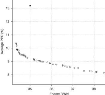
Fig. 12 Pareto-front of the LESO optimization with a population of 80 and 80 iterations. The case Lref is shown as a filled quadrat,
Lopen and Lclosed are not shown because of scale
Fig. 13 Developing of the solutions during the optimization. The initial population is shown in black, the second in blue, the third in yellow, the 10th in green and the final population in red which is also shown in Fig. 12
Table 3 Sets of x values with the results for the LESO case
Setting f1 (kWh) f2 (%) x1 x2 x3 x4 x5 x6 x7 x8 open L closed L ref L 1 best f L 2 bestf L 83.46 57.57 35.00 34.34 38.44 8.53 27.25 13.19 10.36 8.15 1.00 0.00 1.00 0.19 0.31 1.00 0.00 0.60 0.49 0.99 1.00 0.00 0.80 1.00 0.99 1.00 0.00 1.00 1.00 1.00 1.00 0.00 1.00 0.23 0.68 1.00 0.00 0.30 0.23 0.18 1.00 0.00 0.50 0.97 0.33 1.00 0.00 0.70 0.50 0.74
pareto-front. In the first generations the population is moving fast towards the optimal pareto-front, whereas at the end the movement is dramatically slowing down. With this knowledge the number of generations for future optimizations can be estimated to avoid useless iterations.
The best setting in terms of energy consumption is 1 best f
L
which consumed 34.34 kWh and has an average PPD of 10.36%. One can see that Lref is relatively close to the ideal energy consumption but is lacking average PPD. On the other hand, 2
best f
L which is the best setting for objective f2 (average PPD) does not improve average PPD that much, creating a flat trade-off between the two objectives. It is worth noting again that the occupant does not need to change his clothing in order to adapt to the changes and for that reason the PPD reaches relatively high2 but still acceptable values.
In Table 4 we show how energy consumption (objective
f1) is distributed over the periods. One can see that the minimum energy consumption for the winter can be reached with leaving the blinds open all the time. This makes sense
as the heat gains are maximized and the blinds have no influence on the insulation, which is the opposite result to the Elfenau case. The high-energy consumption during the winter period is due to low radiation and cannot be compensated by any blind controller. In the intermediate and summer cases, one can better see the impact of a good controller. The energy consumption in 1
best f
L is reduced 98% in the intermediate and 99% in the summer period compared to Lopen. By comparing
1 best f
L and Lref there is still an improvement of 39% in the intermediate and 77% in the summer period.
5.1.1 Influence of the parameters
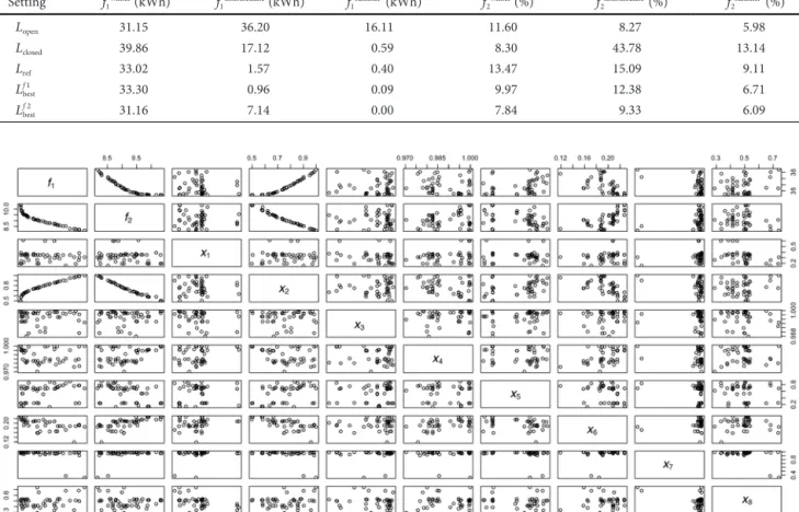
For designing fuzzy systems it is interesting to investigate the influence of the fuzzy parameters on the results. In Fig. 14 we plotted all 8 parameters and the two objectives against each other. Attention must be given to the scale that is individually adapted to the intervals. The parameters, which are strongly correlated to the objectives are x2, x3, x4 and x7,
Table 4 Results for the LESO case separated by periods Setting winter 1 f (kWh) intermediate 1 f (kWh) summer 1 f (kWh) winter 2 f (%) intermediate 2 f (%) summer 2 f (%) open L closed L ref L 1 best f L 2 best f L 31.15 39.86 33.02 33.30 31.16 36.20 17.12 1.57 0.96 7.14 16.11 0.59 0.40 0.09 0.00 11.60 8.30 13.47 9.97 7.84 8.27 43.78 15.09 12.38 9.33 5.98 13.14 9.11 6.71 6.09
Fig. 14 All 8 variables of the LESO optimization and the two objectives of the final population are plotted against each other. By doing this relations between the decision variables and the objectives can be detected and the solutions can be better understood. For example, there is a connection between f1, f2 and x2 and also f1, f2 and x7 are related. One has to take care about the scale which is adapted to each set of data
where x2 is significant as it is not close to 1.00 but rather varies according to the objectives. That means that x2 which corresponds to
If Season is winter and Iglob is high then α=x2
is a crucial parameter for adapting the objectives. On the other hand, the parameters x1, x5 seem to be more randomly distributed. The two rules for the parameters are:
If Season is winter and Iglob is night then α=x1 If Season is summer and Iglob is night then α=x5 Both parameters correspond to Iglob is night and as the textile blinds do not have any affect on the insulation of the building a change in the parameters would not change the result and so the optimization procedure finds no pressure in moving the parameters in any direction.
5.2 Residential apartment building in Elfenau
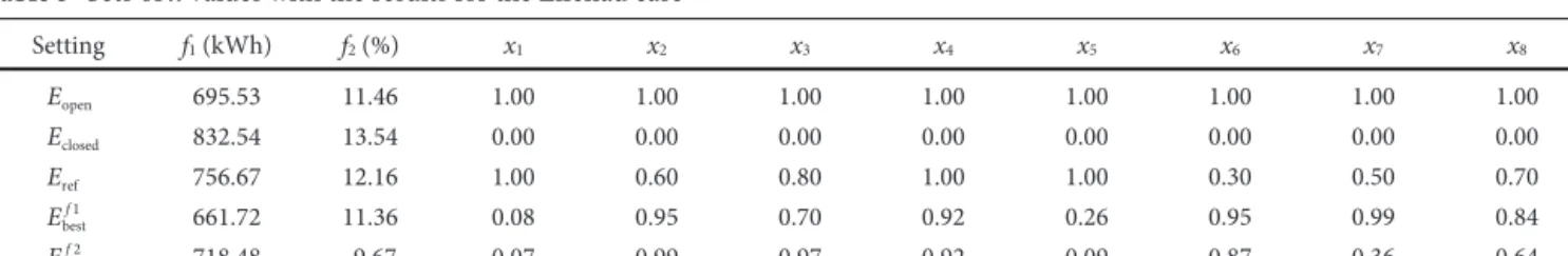
The comparable results can be found in Table 5, the pareto- front of the best population is shown in Fig. 15 together with Eref the solution with the reference setting and Eopen. In the most energy efficient solution, best1
f
E , only 661.72 kWh of energy is consumed for heating during the defined period and the average PPD was at 11.36%. The best value for the average PPD was reached at 9.67% with 2
best f
E and an energy consumption of 718.48 kWh.
The distribution of energy consumption among the three periods is shown in Table 6. Because of a U-value of 0.9 of the roller blinds it was possible to achieve less energy consumption than in the Eopen setting, this is implemented in 1 best f E and 2 best f
E . In the Elfenau case energy savings are less than in the previously discussed LESO case. By comparing
1 best
f
E with Eopen there are savings of 0.3% (winter), 0.6%
(intermediate) and 17.3% (summer) for the single periods. This may be due to the fact that the windows are not all facing the south facade which is the case at the LESO room. Furthermore, the best energy consumption for the winter period is not reached by 1
best f E rather than 2 best f E . This means, that a combination of these two controllers that would behave like 2 best f E in winter and 1 best f
E in the other two periods would be better and if possible should be found through the optimization procedure. Not finding such a solution means that the fuzzy system is not optimally adaptable to its needs and cannot utilize the full saving potential of the blinds.
Fig. 15 Pareto-front of the Elfenau optimization with a population of 60 and 100 iterations. The case Erefis shown as a filled quadrat
and Eopenas a blank one, Eclosedis not shown because of scale
Table 5 Sets of x values with the results for the Elfenau case
Setting f1 (kWh) f2 (%) x1 x2 x3 x4 x5 x6 x7 x8 open E closed E ref E 1 bestf E 2 best f E 695.53 832.54 756.67 661.72 718.48 11.46 13.54 12.16 11.36 9.67 1.00 0.00 1.00 0.08 0.07 1.00 0.00 0.60 0.95 0.99 1.00 0.00 0.80 0.70 0.97 1.00 0.00 1.00 0.92 0.92 1.00 0.00 1.00 0.26 0.09 1.00 0.00 0.30 0.95 0.87 1.00 0.00 0.50 0.99 0.36 1.00 0.00 0.70 0.84 0.64
Table 6 Results for the Elfenau case separated by periods Setting winter 1 f (kWh) intermediate 1 f (kWh) summer 1 f (kWh) winter 2 f (%) intermediate 2 f (%) summer 2 f (%) open E closed E ref E 1 best f E 2 best f E 493.37 495.85 501.09 491.88 486.87 193.91 293.51 239.51 192.74 203.83 8.24 43.17 15.97 6.81 11.83 10.57 11.28 10.55 10.32 8.67 13.27 17.30 14.94 13.41 11.64 8.73 8.27 8.21 8.29 6.73
6 Conclusions and future work
This paper proposed a combination of a high-level simulation program and an optimizer based on evolutionary algorithms. The LESO one room case and the residential apartment were the two different settings that were compared. It was then shown that for both, the combination is capable of finding solutions that are significantly better than the reference case used. Due to detailed modeling the results can be transferred directly into a real world application. The energy savings found showed the necessity for optimization in this field and the superiority of the resulting solutions in terms of energy and thermal comfort to the man made counterpart. Also the results are only suitable for that specific setup, whereas this approach is capable of assessing the saving potential while keeping in mind the comfort of the occupants. This makes it possible to benchmark different systems and make a statement about the theoretical saving potential of them. One can also compare different types of controllers and may receive a combined pareto-front consisting of the best results by different systems. Then, according to the preferences of the user, the most suitable controller can be chosen. For the design of a new controller, the data of the parameter can be used to identify the critical factors more simply.
6.1 Future work
Future work will involve the investigation of adequate objective functions for visual and thermal comfort of human beings, as this is a crucial point for the acceptance of controllers. Furthermore, specific criteria for a blind controller can also be investigated with this approach and be tested for their efficiency.
References
Achermann M, Zweifel G (2003). RADTEST radiant cooling and heating test cases. A report of Task 22, Subtask C. Building Energy Analysis Tools. Comparative Evaluation Tests, IEA International Energy Agency, Solar Heating and Cooling Programme. Altherr R, Gay J-B (2002). A low environmental impact anidolic
facade. Building and Environment, 37: 1409 − 1419.
Calvino F, La Gennusa M , Rizzo G, Scaccianoce G (2004). The control of indoor thermal comfort conditions: introducing a fuzzy adaptive controller. Energy and Buildings, 36: 97 − 102. Coello Coello CA, Van Veldhuizen DA, Lamont GB (2002).
Evolutionary Algorithms for Solving Multi-Objective Problems. Dordrecht: Kluwer Academic Publishers.
Crawley DB, Hand JW, Kummert M, Griffth, BT (2005). Contrasting the capabilities of building energy performance simulation programs. In: Proceedings of the 9th IBPSA conference, pp. 231 − 238.
Deb K (2000). Multi-Objective Optimization Using Evolutionary Algorithms. New York: Wiley.
Deb K, Pratap A, Agarwal S, Meyarivan T (2002). A fast and elitist multiobjective genetic algorithm: NSGA-II. IEEE Transactions on Evolutionary Computation, 6: 182 − 197.
Dounis AI, Manolakis DE (2001). Design of a fuzzy system for living space thermal comfort regulation. Applied Energy, 69: 119 − 144. Fanger PO (1972). Thermal Comfort. New York: McGraw-Hill. Galasiu AD, Atif MR, MacDonald RA (2004). Impact of window
blinds on daylight-linked dimming and automatic on/off lighting controls. Solar Energy, 76: 523 − 544.
Guillemin A (2003). Using genetic algorithms to take into account user wishes in an advanced building control system. Ph.D Thesis, the University of Lausanne.
Guillemin A, Molteni S (2002). An energy-efficient controller for shading devices self-adapting to the user wishes. Building and Environment, 37: 1091 − 1097.
Herrera F, Lozano M, Verdegay J (1995). Tuning fuzzy logic controllers by genetic algorithms. International Journal of Approximate Reasoning, 12: 299 − 315.
Jian W, Cai W (2000). Development of an adaptive neuro-fuzzy method for supply air pressure control in HVAC system. 2000 IEEE International Conference on Systems, Man, and Cybernetics, 5: 3806 − 3809.
Kolokotsa D (2003). Comparison of the performance of fuzzy controllers for the management of the indoor environment. Building and Environment, 38: 1439 − 1450.
Kolokotsa D, Tsiavos D, Stavrakakis GS, Kalaitzakis K, Antonidakis E (2001). Advanced fuzzy logic controllers design and evaluation for buildings, occupants thermalvisual comfort and indoor air quality satisfaction. Energy and Buildings, 33: 531 − 543. Lah MT, Zupancic B, Peternelj J, Krainer A (2006). Daylight illuminance
control with fuzzy logic. Solar Energy, 80: 307 − 321.
Leigh JP, Markowitz SB, Fahs M, Shin C, Landrigan, PJ (1997). Occupational injury and illness in the United States estimates of costs, morbidity and mortality. Archives Internal Medicine, 157: 1557 − 1568.
Olesen BW (2004). International standards for the indoor environment. Indoor Air, 14: 18 − 26.
Page J, Robinson D, Morel N, Scartezzini J-L (2008). A generalised stochastic model for the prediction of occupant presence. Energy and Buildings, 40: 83 − 98.
Reinhart C (2004). Lightswitch-2002: a model for manual and automated control of electric lighting and blinds. Solar Energy, 77: 15 − 28.
Sahlin P, Eriksson L, Grozman P, Johnsson H, Shapovalov A, Vuolle M (2004). Whole-building simulation with symbolic DAE equations and general purpose solvers. Building and Environment, 39: 949 − 958.
Sugeno M (1985). Industrial Applications of Fuzzy Control. New York: Elsevier.