Improving accuracy and efficiency of CFD predictions of propeller open water performance

Publisher’s version / Version de l'éditeur:

Vous avez des questions? Nous pouvons vous aider. Pour communiquer directement avec un auteur, consultez la première page de la revue dans laquelle son article a été publié afin de trouver ses coordonnées. Si vous n’arrivez Questions? Contact the NRC Publications Archive team at

PublicationsArchive-ArchivesPublications@nrc-cnrc.gc.ca. If you wish to email the authors directly, please see the first page of the publication for their contact information.

https://publications-cnrc.canada.ca/fra/droits

L’accès à ce site Web et l’utilisation de son contenu sont assujettis aux conditions présentées dans le site LISEZ CES CONDITIONS ATTENTIVEMENT AVANT D’UTILISER CE SITE WEB.

Journal of Naval Architecture and Marine Engineering, 16, 1, pp. 1-20,

2019-06-30

READ THESE TERMS AND CONDITIONS CAREFULLY BEFORE USING THIS WEBSITE. https://nrc-publications.canada.ca/eng/copyright

NRC Publications Archive Record / Notice des Archives des publications du CNRC :

https://nrc-publications.canada.ca/eng/view/object/?id=c5bf6612-8c63-44b7-a5b4-59cfc27a5af0

https://publications-cnrc.canada.ca/fra/voir/objet/?id=c5bf6612-8c63-44b7-a5b4-59cfc27a5af0

NRC Publications Archive

Archives des publications du CNRC

This publication could be one of several versions: author’s original, accepted manuscript or the publisher’s version. / La version de cette publication peut être l’une des suivantes : la version prépublication de l’auteur, la version acceptée du manuscrit ou la version de l’éditeur.

For the publisher’s version, please access the DOI link below./ Pour consulter la version de l’éditeur, utilisez le lien DOI ci-dessous.

https://doi.org/10.3329/jname.v16i1.34756

Access and use of this website and the material on it are subject to the Terms and Conditions set forth at

Improving accuracy and efficiency of CFD predictions of propeller open

water performance

Journal of Naval Architecture and Marine Engineering June, 2019

http://dx.doi.org/10.3329/jname.v16i1.34756

1813-8535 (Print), 2070-8998 (Online) © 2019 ANAME Publication. All rights reserved. Received on: November 2017

IMPROVING ACCURACY AND EFFICIENCY OF CFD

PREDICTIONS OF PROPELLER OPEN WATER PERFORMANCE

M. F. Islam

and F. Jahra

1

Oceanic Consulting Corporation, mfis07@gmail.com (Currently employed at the National Research Council, Canada) 2

Fleetway Inc., jahra.fatima@fleetway.ca

Abstract:

This research proposes mesh and domain optimization strategies for a popular Computational Fluid Dynamics (CFD) technique to estimate the open water propulsive characteristics of fixed pitch propellers accurately and time-efficiently based on examining the effect of various mesh and computation domain parameters. It used a Reynolds-Averaged Navier-Stokes (RANS) solver to predict the propulsive performance of a fixed pitch propeller with varied meshing, simulation domain and setup parameters. The optimized mesh and domain size parameters were selected using Design of Experiments (DoE) methods enabling simulations in a limited memory and in a timely manner without compromising the accuracy of results. The predicted thrust and torque for the propeller were compared to the corresponding measurements for determining the prediction accuracy. The authors found that the optimized meshing and setup arrangements reduced the propeller opens simulation time by at least a factor of six as compared to the generally popular CFD parameter setup. In addition, the accuracy of propulsive characteristics was improved by up to 50% as compared to published simulation results. The methodologies presented in this paper can be similarly applied to other simulations such as calm water ship resistance, ship propulsion etc. to systematically derive the optimized meshing arrangement for simulations with minimal simulation time and maximum accuracy. This investigation was carried out using a commercial CFD package; however, the findings can be applied to any RANS solver.

Keywords: CFD, RANS methods, mesh optimization, design of experiments, propulsive characteristics,

propeller thrust and torque.

NOMENCLATURE

v

u ,

uii Velocity in the ith direction β Coefficient of thermal expansion T Propeller thrust ν Kinematic viscosity

Q Propeller torque ρ Water density

n Propeller rotational speed k Turbulent kinetic energy

D Propeller diameter ω Turbulent dissipation rate

VA Propeller advance speed in the direction of

carriage motion νt Turbulent viscosity

KT Propeller thrust coefficient ηProp Propeller efficiency

1. Introduction

One of the drawbacks of any RANS solver is the huge requirements of proper mesh generation effort and consequential computational time to solve the domain. One important requirement before carrying out a CFD computation is mesh generation within a domain in which the subject geometry is present. Often, for propeller simulation, a domain size is selected arbitrarily such that the domain boundaries are sufficiently away from the propeller. In addition, multiple refinement zones are used to the domain to capture flow dynamics around the leading and trailing edges of the blades and possible flow separations. The sizes of these refinement zones are picked based on experience or using trial and error approaches. These often result in unnecessarily large domain

and refined zone sizes, hence a large number of cells. Generally, a mesh dependency/sensitivity study is carried out to understand the influence of mesh size and refinement on the simulation results. It is often very expensive and time consuming to obtain a completely mesh independent solution, particularly if the mesh size is reduced erratically. Achieving a suitable mesh density for a specific problem with acceptable computational time and numerical accuracy has remained a major research topic in the CFD.

The common practice in propulsion prediction studies is to perform local refinement near the propeller blades and along the propeller axis in the form of a cylinder with diameter slightly larger than the propeller. Nevertheless, a coarser mesh is maintained at the far field fluid domain. A mesh dependency study is generally carried out in order to ensure that the solution is independent of the mesh size. This is usually achieved through a gradual reduction in mesh size until a small difference in the thrust and / or torque coefficient predictions between two successive mesh refinements is reached. This process continues until the difference in the drag coefficient is below 0.005 or less than 5%. However, this does not necessarily confirm optimum domain and refinement zones. In addition, a steady state simulation is a common practice with 2000 to 5000 iterations. This approach often results in a numerical accuracy in the range of 2% to 10% and a simulation time in the range of 5 to 12 hours (depending on the number of CPU cores (processors) used for the simulation).

Funeno (1999 and 2002) simulated the current around a highly skewed propeller using an unstructured mesh. The results had good correspondence experiment data for steady state and unsteady flow, but this method was complicated and time consuming. Martínez-Calle (2002) simulated the propeller using a k-epsilon turbulent method in steady state open water conditions. Overall, the results were acceptable but there was approximately 30% error in prediction of torque coefficient. Takekoshi (2003) simulated the propeller using a standard k-omega turbulent method in open water and steady state conditions. For simulation of propeller geometry and its surrounding fluid, he used the propeller symmetry and simulated only one blade and compared the results of experiments with his simulated results, which resulted in a 15 percent error in the simulation results, relative to the experiments. Nasika et al. (2010) presented a methodology to predict the propeller hydrodynamic performance using a finite volume numerical modeling approach such as the commercial code ‘Fluent’. The authors claimed that the results were comparable to the experimental results with the benefits of decreased time and cost, details of the flow around the propeller with pressure and velocity contours, with no limitation in velocity flow and model size. However, it should be noted that the error in thrust and torque predictions were up to 20%. The analysis of the results from the studies above shows that there is a need for further improvement of prediction techniques for propeller characteristics.

The application of design of experiment techniques to obtain optimized domain setup parameters for propeller simulations has not been reported before. Ahmed et al. (2010) presented a mesh optimization strategy for accurately estimating the drag of a ground vehicle. This study was based on examining the effect of different mesh parameters using a Design of Experiments (DoE) method. A simplified car model at three scales was investigated and compared with results from the MIRA model wind tunnel (Ahmed et al. 2010). Scaling the optimized mesh size with the length of car model was successfully used to predict the drag of the other car sizes with reasonable accuracy. The current study was inspired by this study. Islam and Lye (2009) presented the application of DOE methodologies to obtain simplified models to predict the propulsive characteristics of a propeller.

The present study provides guidelines for generating domain and meshing arrangements for solving hydrodynamic flow over a propeller model. An optimization study has been carried out to find out the combination of domain, refinement zone and mesh sizes, which would give the least simulation time, and the most accurate results for propeller performance characteristics using modern statistical design of experiment methodologies. It recommends initial values for different mesh and domain parameters to reduce computation time and memory usage. One propeller was used in the current study termed as the “Base” propeller. The optimization study was carried out using the Base propeller and validated using a “Second” propeller to obtain the optimum domain characteristics that give the least simulation time and most accurate predictions compared to the corresponding measurements of propulsive characteristics. Parameters, named outer domain size, inlet and outlet distances, inner domain diameter and extent and base mesh size are studied. The surface growth rate, mesh type, number of prism layers and prism layer thickness were assumed constant. The commercial Reynolds-Averaged Navier Stokes (RANS) solver, Star-CCM+ (CD-Adapco 2014), was used to predict the propulsive performance of the propellers at various loading conditions.

Section 2 presents the details of the propeller models used in the research. Section 3 provides a brief overview of the mathematical formulation of various CFD models used in the research. The application of a fractional factorial design to the problem at hand is presented in Section 4. This Section presents the optimization techniques that are applied to the resulting model of the domain characteristics to obtain the least time consuming and most accurate combination of meshing parameters to predict propeller coefficients. Section 5 presents the simulation results and discussions on the validation of the optimized models. A few concluding remarks are presented in Section 6.

2. Propeller Models

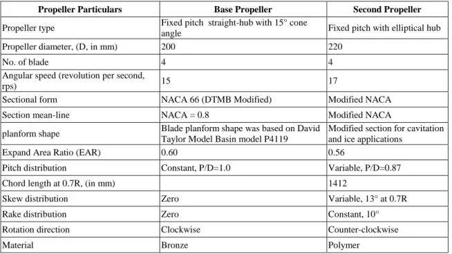
The experiments and numerical analyses included a left-handed model propeller with a hub taper angle of -15°. This propeller was used as the base propeller for the optimization of the domain characteristics and the initial validation of the optimized domain. Another stock propeller was used as a second propeller to validate the optimized domain characteristics. Table 1 presents a description of the geometric characteristics of both propellers. Islam (2009) provides details of the geometry of the propellers. Figure 1 shows the physical and rendered models of the propeller.

Table 1: Geometric characteristics of the base propeller and the second propeller used in the current study

Propeller Particulars Base Propeller Second Propeller

Propeller type Fixed pitch straight-hub with 15° cone

angle Fixed pitch with elliptical hub

Propeller diameter, (D, in mm) 200 220

No. of blade 4 4

Angular speed (revolution per second,

rps) 15 17

Sectional form NACA 66 (DTMB Modified) Modified NACA

Section mean-line NACA = 0.8 Modified NACA

planform shape Blade planform shape was based on David

Taylor Model Basin model P4119

Modified section for cavitation and ice applications

Expand Area Ratio (EAR) 0.60 0.56

Pitch distribution Constant, P/D=1.0 Variable, P/D=0.87

Chord length at 0.7R, (in mm) 1412

Skew distribution Zero Variable, 13° at 0.7R

Rake distribution Zero Constant, 10°

Rotation direction Clockwise Counter-clockwise

Material Bronze Polymer

In the physical model testing of the propellers, the performance characteristics of the propeller were measured and analyzed under different operating conditions using the ITTC recommended procedure, Podded Propulsor Tests and Extrapolation (2002). The dynamometer system measured propeller shaft thrust (T) and propeller shaft torque (Q). In addition, the shaft rotation rate and inflow speeds were also recorded. The experiments were performed in the 200m long towing tank at Ocean, Coastal and River Engineering (NRC-OCRE) facilities in St. John’s. The propeller forces are presented in the form of traditional non-dimensional coefficients as defined in Table 2 (Islam 2009).

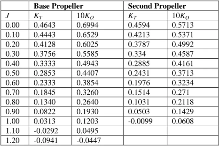
Table 3 presents the open water propulsive characteristics of the base propeller and the second propeller obtained from the open water experiments. The thrust and torque coefficient values decrease as the inflow speed increases at a constant propeller shaft rotation rate (rps). For the measurements and the simulations, the shaft rotational speed for the base propeller and the second propeller were 15 rps and 17 rps, respectively.

Figure 1: The Base and the Second propellers; Left- the physical and rendered models of the Base propeller, Right- the physical and rendered models of the Second propeller

Table 2: Data reduction equations and definitions of parameters

Performance Characteristics Data Reduction Equation KT – propeller thrust coefficient T/n2D4

10KQ – propeller torque coefficient

5 2

/ 10Q



J – propeller advance coefficient

V

/

nD

ηProp – propeller efficiency J/2





Table 3: The measured open water propulsive characteristics of the Base and the Second propellers

Base Propeller Second Propeller

J KT 10KQ KT 10KQ 0.00 0.4643 0.6994 0.4594 0.5713 0.10 0.4443 0.6529 0.4213 0.5371 0.20 0.4128 0.6025 0.3787 0.4992 0.30 0.3756 0.5585 0.334 0.4587 0.40 0.3333 0.4943 0.2885 0.4161 0.50 0.2853 0.4407 0.2431 0.3713 0.60 0.2333 0.3854 0.1976 0.3234 0.70 0.1845 0.3260 0.1514 0.271 0.80 0.1340 0.2640 0.1031 0.2118 0.90 0.0822 0.1930 0.0503 0.1429 1.00 0.0313 0.1203 -0.0099 0.0608 1.10 -0.0292 0.0495 1.20 -0.0941 -0.0447

3. Simulation Methodology

A general discussion on the mathematical background used in the RANS solver and propeller simulation method used in the current work is presented in this section.

3.1

Governing equations

The fluid is assumed to be incompressible. The governing equations are for mass and momentum conservation. Using the Reynolds averaging approach, the Navier-Stokes equations can be stated as in Equation 1 and 2:

0







x

u

 

_





























































j

u

i

u

x

u

j

x

i

x

p

j

u

i

u

j

x

i

u

t









where 



3.2

Turbulence model

The two-equation standard k-ω model, which was popularized by Wilcox (1998), incorporates modifications for low-Reynolds-number effects, compressibility, and shear flow spreading. This model is an empirical model where one equation involves the turbulence kinetic energy (k) representing the velocity scale, and the other takes the turbulent dissipation rate (ω) into account representing the length scale. The standard two-equation k-ω model turbulence model accounting for the effect on turbulence is provide in Equation 3 through 6:

 

 

 

 

where σk and σω are the turbulent Prandtl numbers for k and ω, respectively, and

𝑃𝑘≈ 𝜇𝑡(𝜕𝑢_𝜕𝑥𝑖 𝑗+ 𝜕𝑢_𝑗 𝜕𝑥_𝑖) 𝜕𝑢_𝑖 𝜕𝑥_𝑗 (5)

is the rate of production of turbulent kinetic energy. The turbulent viscosity, µt, is computed by combining k and ω as follows:    _t * k (6) The coefficient *damps the turbulent viscosity causing a low-Reynolds-number correction (Menter 1994).

3.3

Propeller simulation method

The rotation of the propeller in the fluid environment is modelled in a steady-state manner by using Moving Reference Frame (MRF) method in RANS solver. A rotating reference frame is a rotating frame of reference that can be applied to regions to generate a constant grid flux. This approach gives a solution that represents the time-averaged behavior of the flow, rather than the time-accurate behavior.

In this case, governing equations are solved with additional acceleration terms. The computational domain is divided into stationary and moving frames. For an arbitrary point in solution field, the absolute velocity, v and relative vr _{can be defined by the following relation:}

 

v

v_r  ₍₇₎

where r is the position vector from the origin of the moving frame and  is the angular velocity vector. The governing equations of fluid flow in a moving reference frame can be written in two different ways: absolute velocity formulation or relative velocity formulation. The mass and momentum equation in the relative velocity formulation can be stated as:

 





 













.

2

)

(

)

(

v







v

v







v











r





p





t

where













is the centripetal acceleration, Ferziger and Peric (2002).

All computations reported here are performed using the commercial CFD software Star-CCM+. It is based on a finite volume (FV) method and starts from the conservation equations in integral form. With appropriate initial and boundary conditions and by means of a number of discrete approximations, an algebraic equation system solvable on a computer is obtained. First, the spatial solution domain is subdivided into a finite number of contiguous control volumes (CVs) which were of an arbitrary polyhedral shape and were made smaller in regions of rapid variation of flow variables. The governing equations contain surface and volume integrals, as well as time and space derivatives. These are then approximated for each CV and time level using suitable approximations. The solvers also took into account the effects of viscosity and turbulence due to the complex flow pattern around propeller blades.

4. Optimization Methodology

The strategy to reach the optimum meshing arrangement for propeller simulation followed the six stages stated below. A further description of the steps and the outcome of the approach are provided in the following section.

(a) Stage 1: Identify the domain parameters and select the high and low values for each of the domain and mesh parameters;

(b) Stage 2: Design of Experiments using the Fractional Factorial Design and perform the simulations; (c) Stage 3: Statistical analysis of the results for the Factorial Design and screen out the insignificant

parameters;

(d) Stage 4: Mesh parameter optimization using statistical analysis;

(e) Stage 5: Perform additional simulations with the base propeller and using the optimized domain parameters for initial validation of the optimized model; and

(f) Stage 6: Perform simulation with an arbitrary propeller to validate the optimized model using the domain parameters. Note, this stage is currently being carried out, hence not presented in the paper.

4.1

Selection of domain parameters and factorial design

A literature survey showed that for the majority of propeller simulations, a cylindrical outer domain is used with a number of inner cylinders for local mesh refinements. The outer domain generally has 3D to 7D, where D is the propeller diameter. The distance between the rotating frame, which is also the propeller center, and inlet varies between 3D and 6D, while it is between 4D and 10D for the outlet and propeller center frame. For local mesh refinement, it is a recommended practice to use an axial refinement along the propeller axis spanning the length of the domain with a diameter 1.5D to 3D (Nakisa et al., 2010). Some researchers use an additional mesh refinement zone that span the diameter of the external domain and extended along the axis for 0.5D to 2D concentric to the propeller, Shamsi and Ghassemi (2013). The domain parameters typically used for a propeller is summarized in Table 4.

Table 4: The popular domain parameters for the base propeller

Domain Parameters Base Propeller

Outer Diameter (OD) 5

Inlet Distance from propeller centre (IDist) 4 Outlet Distance from propeller centre (ODist) 8 Refinement Zone I Diameter, this extends the

main domain length (ID Dia) 2

Refinement Zone II Extent, this extends the

main domain diameter (ID Ext) 1.5

Mesh Base Size 100

In the current research, a total of six input domain and meshing parameters are selected for the optimization study, namely: outer domain size, inlet and outlet distances, inner domain diameter and extent and base mesh

size. A fractional factorial design (FFD) (Islam and Lye, 2009) was used to design the experiments to minimize the runs. The factors are given in Table 5 with the corresponding low and high values to be considered in the FFD design. The ranges of each of the input variables are selected based on what has been used in predicting propeller characteristics using RANS solver in the literature. With six factors, the half- fractional two-level factorial design (26-1) requires a combination of experimental 32 runs or calculation points. The design is a Resolution V design, which means that all main effects and two-factor interactions can be estimated without ambiguity, Montgomery (2005). Note, there are other parameters such as free-stream turbulence intensity, boundary conditions, and propeller rotation rate could also be parameters in the design. Further details of design of experiment techniques and two-level fractional factorial design can be found in Montgomery (2005) and Islam and Lye (2009).

Table 5: The variables of control with their ranges (low and high values)

Factors (multiplication of Base propeller diameter) Notation Low (-1) High (+1)

A Outer/Main Domain Diameter, Cylindrical Domain OD 2 4

B Inlet Distance from Propeller Centre IDist 2 4

C Outlet Distance from Propeller Centre ODist 3 8

D Refinement Zone I Diameter, this extends the main domain

length ID Dia 1.25 2

E Refinement Zone II Extent, this extends the main domain

diameter ID Ext 0.5 1.5

F Mesh Base Size, original base size = 0.1 m Base Size 50 250

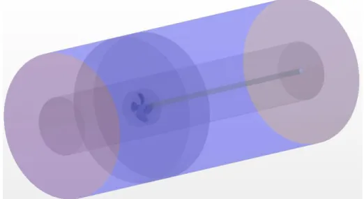
Figure 2: The popular mesh block model of simulation field for the base propeller

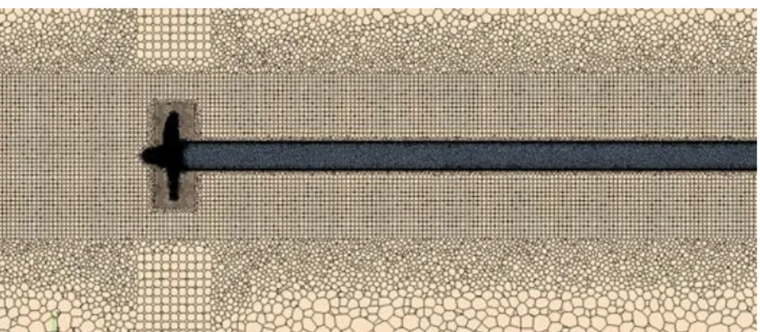
The experimental design requires that the RANS solver is used to model the base propeller in a solution domain with changed dimension parameters. The relative position of each of the sub-domains with respect to the propeller center remained the same. Figure 2 and Figure 3 show the 3D computational domain for the base propeller and for the second propeller, respectively, with the popular domain and meshing factors. Figure 4 and Figure 5 show the volume mesh for the propeller on a vertical plane through the propeller center for the base propeller and for the second propeller, respectively, in its popular setup. Unstructured grid was used, which results in a smoother discretization near the leading and trailing edge of both propellers, see Figure 6.

Figure 4: The vertical plane showing the volume mesh around the base propeller using the popular setup

Figure 5: The vertical plane showing the volume mesh around the second propeller using the popular setup

Figure 6: The fine mesh around the leading and trailing edges of the blades of the base propeller (left) and of the second propeller (right) using the popular setup

The 32 run combinations for the 26-1 design and the responses are shown in Table 6. A total of 32 simulation files were developed using the domain parameters presented in Table 5. For each case, the volumetric mesh was generated in the domain using polyhedral cells. The meshing arrangements around the base propeller in a vertical plane for the FFD combination 1 and 32 are shown in Figure 7, and in Figure 8, respectively.

For each of the simulations, the inlet boundary condition for the fixed frame is set as a velocity inlet with a constant velocity profile. The outlet boundary condition was set as a pressure outlet. The propeller blades, hub and shaft are assumed as wall boundary conditions. In each of the simulations, the governing equations are solved by the finite volume method. The SIMPLE algorithm is used to solve the pressure-velocity coupling equations. The second order upwind discretization scheme is utilized for the momentum, turbulent kinetic energy, and turbulent dissipation rate. The rotation of the propeller is modelled using moving reference frame method and turbulence is modelled by Menter’s SST k-ω method, Menter (1994). The relative meshing arrangements for each of the refinement zones were kept the same for each simulation. Also, the simulation boundary conditions and kinematics were unchanged between the simulations. All simulations in the FFD study were carried out at uniform inlet velocity of 1.5 m/s with the propeller rotating at 15 rps (J=0.5). The measured thrust and torque of the base propeller in the corresponding open water model test condition were 102.7 N and 3.17 N-m, respectively.

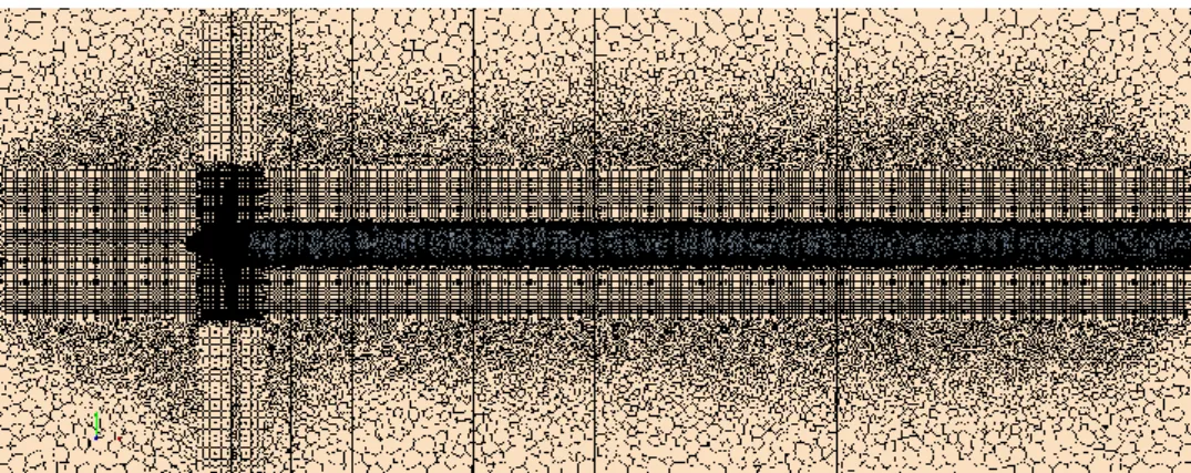
Figure 7: The vertical plane showing the volume mesh around the base propeller using the FFD domain setup 1 in Table 6

Figure 8: The vertical plane showing the volume mesh around the base propeller using the FFD domain setup 32 in Table 6

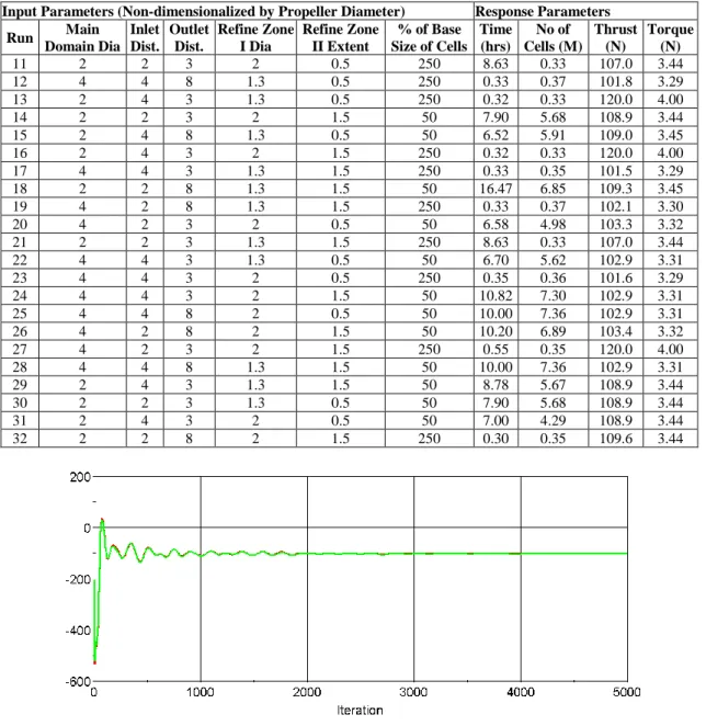
Table 6: Fractional Factorial Design (FFD) Data Sheet

Input Parameters (Non-dimensionalized by Propeller Diameter) Response Parameters Run Main Domain Dia Inlet Dist. Outlet Dist. Refine Zone I Dia Refine Zone II Extent % of Base Size of Cells Time (hrs) No of Cells (M) Thrust (N) Torque (N) 1 4 2 8 1.3 0.5 50 4.97 6.96 103.5 3.32 2 2 4 8 1.3 1.5 250 0.28 0.35 108.1 3.46 3 4 2 8 2 0.5 250 10.67 7.54 109.4 3.45 4 4 2 3 1.3 0.5 250 0.55 0.34 120.0 4.00 5 4 4 8 2 1.5 250 0.38 0.40 101.0 3.30 6 4 2 3 1.3 1.5 50 6.58 4.98 103.3 3.32 7 2 2 8 1.3 0.5 250 0.32 0.35 109.9 3.45 8 2 4 8 2 1.5 50 6.52 5.91 109.0 3.45 9 2 4 8 2 0.5 250 0.33 0.35 108.5 3.43 10 2 2 8 2 0.5 50 4.50 6.85 109.2 3.45

Input Parameters (Non-dimensionalized by Propeller Diameter) Response Parameters Run Main Domain Dia Inlet Dist. Outlet Dist. Refine Zone I Dia Refine Zone II Extent % of Base Size of Cells Time (hrs) No of Cells (M) Thrust (N) Torque (N) 11 2 2 3 2 0.5 250 8.63 0.33 107.0 3.44 12 4 4 8 1.3 0.5 250 0.33 0.37 101.8 3.29 13 2 4 3 1.3 0.5 250 0.32 0.33 120.0 4.00 14 2 2 3 2 1.5 50 7.90 5.68 108.9 3.44 15 2 4 8 1.3 0.5 50 6.52 5.91 109.0 3.45 16 2 4 3 2 1.5 250 0.32 0.33 120.0 4.00 17 4 4 3 1.3 1.5 250 0.33 0.35 101.5 3.29 18 2 2 8 1.3 1.5 50 16.47 6.85 109.3 3.45 19 4 2 8 1.3 1.5 250 0.33 0.37 102.1 3.30 20 4 2 3 2 0.5 50 6.58 4.98 103.3 3.32 21 2 2 3 1.3 1.5 250 8.63 0.33 107.0 3.44 22 4 4 3 1.3 0.5 50 6.70 5.62 102.9 3.31 23 4 4 3 2 0.5 250 0.35 0.36 101.6 3.29 24 4 4 3 2 1.5 50 10.82 7.30 102.9 3.31 25 4 4 8 2 0.5 50 10.00 7.36 102.9 3.31 26 4 2 8 2 1.5 50 10.20 6.89 103.4 3.32 27 4 2 3 2 1.5 250 0.55 0.35 120.0 4.00 28 4 4 8 1.3 1.5 50 10.00 7.36 102.9 3.31 29 2 4 3 1.3 1.5 50 8.78 5.67 108.9 3.44 30 2 2 3 1.3 0.5 50 7.90 5.68 108.9 3.44 31 2 4 3 2 0.5 50 7.00 4.29 108.9 3.44 32 2 2 8 2 1.5 250 0.30 0.35 109.6 3.44

Figure 9: The predicted thrust for the base propeller simulation at advance coefficient, J=0.5

The simulations were run using STAR-CCM+ version 11.04 and the computation was carried out on Intel Core 2 Duo 3GHz processors with 16GB RAM. At least 2000 steady state iterations were completed for each simulation. As shown in Figure 9, the predicted value converges before 2000 iterations are completed in the steady state simulations. Any further increase in the iterations does not improve the results. Also, the residuals in the simulations reach an acceptable low value after 2000 iterations are completed (see Figure 10). The thrust and torque coefficients obtained from the CFD models were validated with experimental results, see Section 6.

4.2

Statistical analysis of the FFD

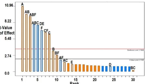
The focus of this analysis is to determine the most significant factors among the six factors in Table 5 for the simulation time and accuracy of thrust and torque of the propeller as compared to the corresponding measurements. Design Expert® 7.03 from Statease, a stand-alone software for design of experiments, was used to design the experiments and analyze the results. It was found that all six parameters were significant directly or in the form of interactions to define the response parameters, see Figure 11. This is a plot of the ordered absolute value of the effects estimates. The model for thrust obtained from the fractional factorial design in physical units is given in Equation 10. The model for the torque is given in Equation 11. This simple linear model for thrust gave a R2 value of about 96% and predicted R2 of about 90%. The torque model gave a R2 value of about 99% and predicted R2 of about 96%. The high number of R2 value means high accuracy of the predicting model, Montgomery (2005). Note these models are to predict propeller thrust and torque when the simulation domain parameters are kept within the ranges used to develop the models; see Table 5.

Figure 11: The Pareto Chart showing the significant domain setup parameters for propeller thrust prediction

Thrust (T) =+4.40373-6.42792 * OD-8.99829 * Dist- 7.09632 * ODist+8.71033 * ID Dia+15.55829 * ID Ext+0.13178 * Base Size+2.91042 * OD * IDist+2.24017 * OD * ODist-0.065826 * OD * Base Size+2.11829 * IDist * ODist-0.055337 * IDist * Base Size+5.81939E-003 * ODist * Base Size-9.24146 * ID Dia * ID Ext-0.69960 * OD * IDist * ODist+0.020486 * OD * IDist * Base Size

(10)

Torque (Q)=+9.15846-9.86346 * OD-11.36656 * IDist-8.77371 * ODist+11.93103 * ID Dia+20.14026 * ID Ext+0.15171 * Base Size+3.85251 * OD * IDist+2.82000 * OD * ODist -0.079085 * OD * Base Size+2.69254 * IDist * ODist-0.072463 * IDist * Base Size+9.03500E-003 * ODist * Base Size-12.23744 * ID Dia * ID Ext-0.91550 * OD * IDist * ODist+0.025463 * OD * IDist * Base Size

(11)

Numerical optimization is carried out using the FFD data set to obtain an optimized combination of domain setup parameters with the objective to obtain the least amount of simulation time and most accurate thrust and torque predictions. The accuracy of the thrust and torque is defined as the percentage difference between the measured and predicted values. The numerical optimization routine offered in Design Expert® 7.03 was used for this purpose. Table 7 presents the domain setup parameters for two optimized setups obtained from the analysis. Setup I was obtained using the criteria for least simulation time and setup II was obtained without setting up any time criteria. In both setup the criteria of maximum accuracy in thrust and torque prediction was

set. The meshing arrangements around the base propeller in a vertical plane for the optimized domain parameters in Setup I and Setup II are shown in Figure 12, and in Figure 13, respectively.

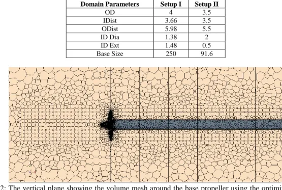
Table 7: The optimized domain parameters for the propeller simulations

Domain Parameters Setup I Setup II

OD 4 3.5 IDist 3.66 3.5 ODist 5.98 5.5 ID Dia 1.38 2 ID Ext 1.48 0.5 Base Size 250 91.6

Figure 12: The vertical plane showing the volume mesh around the base propeller using the optimized domain setup I

Figure 13: The vertical plane showing the volume mesh around the base propeller using the optimized domain setup II

5. Results and Discussion

5.1

Open water performance using traditional domain setup

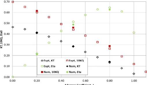
The measurements and predictions of the open water characteristics of the base propeller using the popular domain setup are presented in Figure 14 and in

Table 8. In the popular domain and meshing arrangement, the predicted thrust and torque were within 2% and 4% of the measurements, respectively. Propeller thrust is slightly under-predicted, while the propeller torque is over-predicted. In the RANS simulation, the flow is assumed fully turbulent whereas the model experiments primarily occur in transient flow conditions. This may causes higher skin friction on the blades in the prediction compared to the measurements. A similar comparison for the second propeller is presented in Figure 15 and in

Table 8. Similar to the base propeller, the thrust is slightly under-predicted, while the propeller torque is over-predicted. However, the predicted thrust and torque were within 3% and 9% of the corresponding measurements. The simulation time for each of the data points for both propellers was approximately 2 hours.

Figure 14: Measurements and predictions for open water characteristics of the Base propeller. The simulations were completed using the popular domain setup (1.85M cell, 2.05 hours for each simulation)

Figure 15: Measurements and predictions for open water characteristics of the Second propeller. The simulations were completed using the popular domain setup (2.23M cell, 2.30 hours for each simulation)

5.2

Open water performance using optimized domain setup

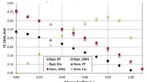
The measurements and predictions of the open water characteristics of the base propeller using the two optimized domain setups are presented in Figure 16 and in Figure 17. In both optimized domain and meshing arrangements, the predicted thrust and torque were within 2% and 3% of the measurements, respectively. In both cases, both thrust and torque were slightly over-predicted. This means an increase in prediction accuracy of approximately 10% and 25% for thrust and torque using the optimized setup I over the popular setup. The simulation time for the base propeller using the popular setup was approximately 6 times higher than using the optimized setup I. However, the simulation time was approximately the same to that using the optimized setup II.

Figure 16: Measurements and predictions for open water characteristics of the Base propeller. The simulations were completed using the optimized domain setup I (0.37M cell, 0.55 hours for each simulation)

Figure 17: Measurements and predictions for open water characteristics of the Base propeller. The simulations were completed using the optimized domain setup II (2.11M cell, 2.15 hours for each simulation)

Figure 18: Measurements and predictions for open water characteristics of the Second propeller. The simulations were completed using the optimized domain setup I (0.39M cell, 0.36 hours for each simulation)

For the Second propeller, the predicted propulsive characteristics as compared to that from the measurements for optimized setup I are presented in Figure 18 and in Table 8. The predicted thrust and torque were within 3% and 5% of the measurements, respectively. This means an increase in prediction accuracy of approximately 10% and 45% for thrust and torque using the optimized setup I over the popular setup. The thrust is under-predicted, while the propeller torque is over-predicted. Similar to the base propeller, the simulation time for the second propeller using the popular setup was approximately 6 times higher than using the optimized setup I.

Table 8: Comparison of measured and prediction propulsive characteristics of the base and the second propellers for various simulation scenarios

Simulation Scenario Predicted Propulsive Characteristics % Difference between Measurements and

Predictions Steady State Simulation Time

J KT 10KQ KT 10KQ No of

Cells

Hours M

Base Propeller, Popular Domain Setup

0.20 0.4083 0.6139 0.97% -1.62% 2.01 1.85 0.50 0.2833 0.4611 0.42% -2.92% 2.01 1.85 0.80 0.1417 0.2875 -1.64% -3.36% 2.01 1.85 Base Propeller, Optimized Domain Setup I 0.00 0.4783 0.7139 -3.02% -2.07% 0.35 0.37 0.10 0.4489 0.6417 -0.98% 1.60% 0.35 0.37 0.20 0.4094 0.5944 0.73% 1.16% 0.35 0.37 0.40 0.3375 0.5067 -0.90% -1.78% 0.35 0.37 0.50 0.2808 0.4585 0.96% -2.54% 0.35 0.37 0.60 0.2364 0.4058 -0.67% -2.92% 0.35 0.37 0.70 0.1893 0.3479 -1.03% -3.13% 0.35 0.37 0.80 0.1419 0.2840 -1.70% -2.86% 0.35 0.37 0.90 0.0886 0.2132 -1.38% -2.89% 0.35 0.37 1.00 0.0336 0.1339 -0.50% -1.94% 0.35 0.37 1.10 -0.0274 0.0444 -0.40% 0.72% 0.35 0.37 Base Propeller, Optimized Domain Setup II 0.00 0.4775 0.6986 -2.84% 0.12% 2.17 2.11 0.10 0.4542 0.6611 -2.12% -1.18% 2.17 2.11 0.30 0.3772 0.5713 -0.34% -1.82% 2.17 2.11 0.50 0.2897 0.4635 -0.96% -3.25% 2.17 2.11 0.70 0.1939 0.3521 -2.02% -3.73% 2.17 2.11 0.80 0.1436 0.2878 -2.06% -3.40% 2.17 2.11 1.00 0.0356 0.1384 -0.92% -2.59% 2.17 2.11 1.10 -0.0251 0.0486 -0.88% 0.13% 2.17 2.11 Second Propeller, Popular Domain Setup

0.20 0.3755 0.5492 0.69% -8.76% 2.3 2.23 0.50 0.2311 0.4131 2.60% -7.32% 2.3 2.23 0.60 0.1880 0.3541 2.09% -5.38% 2.3 2.23 0.80 0.0903 0.2283 2.79% -2.89% 2.3 2.23 Second Propeller, Optimized Domain Setup I 0.00 0.4610 0.6018 -0.35% -5.34% 0.36 0.39 0.10 0.4209 0.5663 0.10% -5.11% 0.36 0.39 0.20 0.3768 0.5241 0.42% -4.35% 0.36 0.39 0.30 0.3279 0.4865 1.33% -4.87% 0.36 0.39 0.40 0.2816 0.4390 1.50% -4.00% 0.36 0.39 0.50 0.2354 0.3927 1.67% -3.75% 0.36 0.39 0.60 0.1895 0.3431 1.75% -3.45% 0.36 0.39 0.70 0.1429 0.2909 1.84% -3.47% 0.36 0.39 0.80 0.0927 0.2265 2.26% -2.58% 0.36 0.39 0.90 0.0385 0.1615 2.57% -3.26% 0.36 0.39 1.00 -0.0234 0.0851 2.93% -4.26% 0.36 0.39

Figure 19, 20 and 21 present the pressure distribution on backside and face side of the base propeller at J=0.5 obtained using the popular, optimized setup I and optimized setup II, respectively. As observed in the figures that the high pressure is on the face and the low pressure is on the backside. The minimum pressures are located on the leading edge of the propeller blades, close to the tip. It is noted that for the optimized setup I, the magnitude of pressure distribution around the leading edge on the face and backsides of the blades is lower than that obtained using the popular setup. This may be attributed to the coarse mesh around the blades. The distribution between the popular setup and optimized setup II is very similar. The axial velocity distribution and

the velocity vector around the base propeller obtained using the popular and the optimized setup appears very similar, see Figure 22, Figure 23, and Figure 24.

Bladed pressure side Blade suction side

Figure 19: The pressure distribution on the blades of the Base propeller using popular domain setup at advance coefficient, J=0.5

Bladed pressure side Blade suction side

Figure 20: The pressure distribution on the blades of the Base propeller using optimized domain setup I at advance coefficient, J=0.5

Bladed pressure side Blade suction side

Figure 21: The pressure distribution on the blades of the Base propeller using optimized domain setup II at advance coefficient, J=0.5

Figure 22: The velocity distribution and velocity vectors on the propeller plane of the base propeller using popular domain setup at advance coefficient, J=0.5

Figure 23: The velocity distribution and velocity vectors on the propeller plane of the base propeller using optimized domain setup I at advance coefficient, J=0.5

Figure 24: The velocity distribution and velocity vectors on the propeller plane of the base propeller using optimized domain setup II at advance coefficient, J=0.5

Figure 25 and Figure 26 presents the pressure distribution on backside and face side of the second propeller at J=0.6 obtained using the popular and optimized setup, respectively. Similar to the base propeller, high pressure is on the face and low pressure is on the backside is observed. The magnitude of pressure distribution around the leading edge on the face and backsides of the blades is slightly lower than that obtained using the popular setup. This may be attributed to the coarse mesh around the blades. As shown in Figure 27 and in Figure 28, the axial velocity distribution and the velocity vector around the second propeller blades obtained using the popular and the optimized setups are very similar.

Blade pressure side Blade suction side

Figure 25: The pressure distribution on the blades of the second propeller using the popular domain setup at advance coefficient, J=0.6

There is a slight increase in the accuracy of thrust and torque prediction of the base propeller using the optimized setup I with significant reduction in simulation time as comparted to the popular simulation setup. For commercial numerical prediction work using CFD packages, especially in the initial design stage, the optimized meshing arrangement may provide improved prediction of the propeller open water performance in a much lower simulation time. The optimized domain setup may produce the open water performance curves within a few hours whereas it may take over a day to obtain similar curves using the popular domain setup, with both methods producing comparable prediction accuracy. However, in the advanced design stage when the pressure and velocity distributions around propeller blades are required, the popular or optimized setup II may generate the desired results.

Back of the blades Face of the blades

Figure 26: The pressure distribution on the blades of the second propeller using the optimized domain setup at advance coefficient, J=0.6

Figure 27: The velocity distribution and velocity vectors on the propeller plane of the second propeller using popular domain setup at advance coefficient, J=0.6

Figure 28: The velocity distribution and velocity vectors on the propeller plane of the second propeller using the optimized domain setup at advance coefficient, J=0.6

6. Concluding Remarks

This study demonstrated that with mesh and domain optimizations, it is possible to use a desktop computer to make accurate predictions of the propulsive characteristics of fixed pitch propellers in open water. In this study, the optimized mesh and domain size parameters were selected using Design of Experiments (DoE) methods enabling RANS simulations to be carried out in a limited memory environment, and in a timely manner; without compromising the accuracy of results.

With the optimized domain and meshing arrangements for both propellers, the predicted thrust and torque were within 2% and 3% of the measurements, respectively. For both propellers, the simulation time using the popular setup was approximately 6 times higher than using the optimized setup I. For commercial numerical prediction work, especially in the initial design stage, the optimized meshing arrangement may provide improved prediction of the propeller open water performance in a much lower simulation time. The optimized domain setup may produce the open water performance curves within a few hours whereas it may take over a day to obtain similar curves using the popular domain setup, with both methods producing comparable prediction accuracy. However, in the advanced design stage when the pressure and velocity distributions around propeller blades are required, the popular or optimized setup II may generate the desired results.

7. Acknowledgements

The authors are indebted to Oceanic Consulting Corporation to facilitate writing this paper and allow access to all relevant information.

8. References

Funeno, I. (1999): Analysis of Steady Viscous Flow around a Highly Skewed Propeller (in Japanese), Journal of Kansai Society of Naval Architects, No. 231, pp. 1-6. https://dx.doi.org/10.14856/jksna.2002.237_39.

Funeno, I. (2002): On Viscous Flow around Marine Propellers –Hub Vortex and Scale Effect, Proceedings of New S-Tech. 2002 (Third Conference for New Ship and Marine Technology), pp. 17-26.

Martínez-Calle, J. (2002): An Open Water Numerical Model for a Marine Propeller: a Comparison with Experimental Data, Proceedings of the ASME FEDSM’02 2002 Joint US-European Fluids Engineering Summer Conference Montreal, Canada, July 14-18, 9p, https://dx.doi.org/10.1115/FEDSM2002-31187.

Takekoshi, Y. (2003): Simulation of Steady and Unsteady Cavitation on a Marine Propeller Using a RANS CFD Code, Fifth International Symposium on Cavitation (CAV2003) Osaka, Japan, November 1-4.

Nakisa, M., Abbasi, M. J., Amini, A M. (2010): Assessment of Marine Propeller Hydrodynamic Performance in Open Water Via CFD, MARTEC 2010, Dhaka Bangladesh, pp. 35-44.

Ahmad, N.E., Abo-Serie, E., Gaylard, A. (2010): Mesh Optimization for Ground Vehicle Aerodynamics, CFD Letters, Vol 2(1) 2010, 12p.

Islam, M., Lye, L.M. (2009): Combined use of Dimensional Analysis and Modern Experimental Design Methodologies in Hydrodynamic Experiments, Ocean Engineering 36 (2009) 237-247,

https://dx.doi.org/10.1016/j.oceaneng.2008.11.004.

Islam, M.F. (2009): Performance study of podded propulsors with varied geometry and azimuthing conditions, Doctoral Dissertation, Memorial University of Newfoundland, St. John’s, NL, Canada, 245p, http://research.library.mun.ca/8916/.

ITTC – Recommended Procedures (2002): Propulsion, Performance - Podded Propeller Tests and Extrapolation. 7.5- 02-03-01.3, Revision 00.

Wilcox, D.C. (1998): Turbulence Modeling for CFD, 2nd edition, DCW Industries, Inc., La Canada, California,

https://dx.doi.org/10.1017/S0022112095211388

Ferziger, J.H., Peric, M. (2002): Computational Methods for Fluid Dynamics, Springer, www.springer.com/gp/book/9783540420743, https://dx.doi.org/10.1007/978-3-642-56026-2

Menter, F.R. (1994): Two-equation eddy-viscosity turbulence modeling for engineering applications, AIAA Journal, 32(8), pp. 1598-1605, https://doi.org/10.2514/3.12149.

Shamsi, R., Ghassemi, H. (2013): Hydrodynamic analysis of puller and pusher of azipod at various yaw angles, Journal Engineering for the Maritime Environment, Volume: 228, issue: 1, page(s): 55-69,

https://dx.doi.org/10.1177/1475090213481417

Montgomery, D.C. (2005): Design and Analysis of Experiments, Fifth ed. Wiley, New York.