An algorithm for rapid measurement of aberrations in pairs of out-of-focus images

An Algorithm for Rapid Measurement of

Aberrations in Pairs of Out-Of-Focus Images ACHNES

by

Ryan J. Janish

A

A

Submitted to the Department of Physics

L iBRAR E

in partial fulfillment of the requirements for the degree of

Bachelor of Science in Physics

at the

MASSACHUSETTS INSTITUTE OF TECHNOLOGY

June 2012

@ Ryan J. Janish, MMXII. All rights reserved.

The author hereby grants to MIT permission to reproduce and to

distribute publicly paper and electronic copies of this thesis document

in whole or in part in any medium now known or hereafter created.

A uthor

...

00'

...

Department of Physics

May 13, 2012

Certified by...

Paul L. Schechter

William A. M. Burden Professor of Astrophysics

Thesis Supervisor

/

Accepted by ...

Nergis Mavalvala

Thesis Coordinator, Department of Physics

An Algorithm for Rapid Measurement of Aberrations in

Pairs of Out-Of-Focus Images

by

Ryan J. Janish

Submitted to the Department of Physics on May 13, 2012, in partial fulfillment of the

requirements for the degree of Bachelor of Science in Physics

Abstract

In this thesis, I present a new technique for measuring the optical aberrations pro-duced by a telescope, with an eye towards future use of these aberration measurements to align wide-field telescopes. This method determines the aberrations by simulta-neously fitting a pair of oppositely defocused images to a mostly analytic model. I develop the model and describe its software implementation in detail, and then re-port on the results of tests with simulated and real data. This technique is able to extract the aberrations from simulated data rapidly and accurately, and it has been used with mixed success to analyze data from the VISTA telescope. With the VISTA data, the algorithm is unable to match small-scale brightness variations in the images. However, it was able to determine aberrations with median accuracies of 0.08 um for coma, 0.08 um for astigmatism, 0.9 um for tilt, and 0.3 um for defocus. It was also quite fast, with an average of 34 iterations until convergence.

Thesis Supervisor: Paul L. Schechter

Acknowledgments

I have been able to complete this thesis only by the gracious help of many people. First of all, I am deeply thankful for my incredible wife, Amanda. Without her support and help, this thesis would certainly never have come to be. I would have never survived the rigors of MIT without her by my side, nor would I have had nearly as good of a time doing so.

I want to thank my advisor, Professor Paul Schechter, who has shown me much patience and guidance during this endeavor. I have learned a lot by working with him, both about the topic of this thesis and about research in general, and by his influence I am certainly a much better scientist now than when I began this work.

I would also like to thank Nancy Savioli, Nancy Boyce, and all of the administra-tors who have helped me navigate the Physics Department, both while completing this thesis and during my entire time here as an undergraduate. It is such friendly and helpful people that make this Department such a great place to be.

Finally, this work makes extensive use of data that I did not collect. I would like to thank Thomas Szeifert, Andreas Kaufer and Magda Arnaboldi for arranging for the VISTA data used in this work to be recorded.

Contents

1 Introduction 2 Image Model

2.1 Aberrations and Imaging 2.2 Brightness . . . . 2.3 Defocus-Only Formulation . . 2.4 Background and Seeing . . . . 2.5 Zernike Coefficients . . . .

3 Algorithms

3.1 Computing Images . . . . 3.2 Fitting for Aberrations . . . . 3.3 Initial Guesses . . . .

4 Performance of the Fit Routine

4.1 Simulated Data . . . . 4.2 VISTA Data . . . .

5 Conclusion

A Formulas

A.1 Illuminated Fraction . . . . A.2 Derivative of Illuminated Fraction . . . . A.3 Hessian Matrix . . . .

6 8 8 10 12 14 15 17 17 18 18 21 21 22 37 38 38 41 43 . . . . . . . . . ... . . . . . . . . . . . . . . . . . . . . . . . . . . . .

A.4 Derivative of the Brightness . . . . 43 A.5 Derivative of the Defocus-Only Position . . . . 45 A.6 Derivative of the Hessian . . . . 47

B Software 49

B.1 Fitting Program. . . . . 49 B.2 Image Program . . . . 56

Chapter 1

Introduction

Wide field telescopes are very sensitive to misalignments and require frequent adjust-ments to ensure that the collected data is of high quality. [ ] The development of fast and accurate alignment techniques is therefore an integral part of fully utilizing the capabilities of large telescopes. This is a particularly important concern in the weak lensing community, as the errors caused by misalignments appear as a false lensing signal and the lensing signal itself is very small. [ ]

To correct a misalignment, one must first measure it. The basic strategy for de-termining misalignments has been to measure the optical aberrations of the telescope in question, which are related to the misaligning displacements and rotations of the mirrors.

[

] Until recently, the most common method for measuring aberrations has been the use of Shack-Hartmann wavefront sensors [ ] [ ], however the latest gen-eration of wide-field telescopes, such as VISTA [ ] and the upcoming LSST [

J

and DES [ ], instead rely on analyzing pairs of out-of-focus images. The VISTA collab-oration was the first to successfully realize this technique, using an image analysis algorithm based on comparing observed images to those simulated with ray-tracing methods. This is time-consuming, as it can take hundreds of iterations for such an algorithm to converge. [ ]

In this thesis, I will present an alternative method that fits out-of-focus image pairs directly to a mostly analytic model, which promises to be a much faster technique. In Chapter 2, I discuss the optical theory behind the model and develop the necessary

mathematics. Chapter 3 focuses on the software implementation of the model, where I discuss at a high level all of the principle algorithms involved. Chapter 4 discusses the results of testing the fit procedure on both simulated data and data taken with the VISTA telescope. Finally, in Appendices A and B, I give all of the practical details necessary for the reader to understand the current progress of this work and be able to develop it further. In Appendix A I derive all of the mathematical results necessary to implement the algorithms discussed in Chapter 3, and in Appendix B I discuss my implementation in more detail and at a much lower level than in Chapter 3.

Chapter 2

Image Model

The goal of this chapter is to develop a model of out-of-focus images of point sources. I begin by briefly introducing some of the theory of optical aberrations, and then use these notions to construct a description of defocused images.

2.1

Aberrations and Imaging

The propagation of light through an optical system can be described in terms of the surfaces of constant phase that lie perpendicular to the light's direction of travel, known as the wavefronts. 1 While there is a wavefront passing through any point in the light's path, of particular interest is the wavefront that passes through the center of the optical system's exit pupil. We can parameterize this wavefront surface as a function w(&,), where w( ,) denotes the distance between the wavefront surface and the plane of the exit pupil at point z, on the pupil. Now, for a perfect optical system, that is, for a system in which the light leaving the pupil is focused to a single focal point located a distance

f

away from the pupil along the optical axis, the central wavefront w(',) must be a spherical cap from a sphere of radius

f

centered on the focal point. For any real optical system, the wavefront w(',) will differ from a perfect spherical cap, and we can therefore characterize the imperfections of an optical system

'I present a very shallow treatment of wavefronts. For those interested, a thorough discussion of wavefront optics can be found in Majahan's text Optical imaging and aberrations, part I [ ]

by the deviation of its wavefront from a sphere. Define the wavefront deviation to be

() = W(',) - Wsphere(Xp) (2-1)

where Wsphere(sp) is the spherical wavefront the system would have if it focused per-fectly and w(',) is the actual wavefront. For simplicity, I will typically refer to W(s,) as just the wavefront.

Describing the imaging process in terms of W(',) is particularly useful for two reasons:

1. W(',) tells us where a ray that crosses the pupil at ', will eventually inter-sect the image plane. If the image point is denoted by si, then (in Cartesian

coordinates):

si

=

f

,W(z,) (2.2)

Rout

where V, indicates the gradient with respect to the pupil position,

f

is the focal length, and R,, is the outer pupil radius.

]

Thus, if we know the function W(',), we can use it to construct a transformation that maps pupil points to image points. Note that the choice of f

/Rt

as a pre-factor is mere convention. This allows us to both have ', be a dimensionless quantity that is normalized to 1 at the outer pupil radius and also let W(',) be measured in units of length.

2. We do know the function W(z,), approximately, and with seven free parameters. For a realistic imaging system, W(s,) is well-approximated by the following third-order polynomial:

W(x,,y

, cX

+C

cyaX

+

CyXP ± cxxpy

± (d + a,)x2 + (d - a.)y2 _{+ 2a x y,}

+ tXxP + tyyp (2.3)

optical aberrations. [ ] Specifically, c, and cy are the coma, ax and a. are the astig-matism, t, and t, are the tilt, and d is the defocus. These parameters are functions

of the physical properties of the imaging system.

Note that the above aberration parameters are not the usual Zernike coefficients. For a conversion to Zernikes, see Section 2.5. By the conventions stated above for the units of W(i,) and ',, all of the aberration parameters are measured in units of length. And in particular, since they are the only dimension-full quantities in the wavefront, we say they are measured in distance of wavefront error.

Combining Equations 2.2 and 2.3 gives an explicit transformation between the pupil and image planes:

Xi = 3c.xx + cXy2 + 2cyxpyp + 2(d + ax)xp + 2ayy + tX (2.4) yi = cYx _{+ 3cyy2 + 2c.xyp + 2ayxp + 2(d - a,)yp + ty}

This transformation completely determines the observed image, provided we know the distribution of rays across the pupil. Now, if we restrict attention to the case of imaging a distant point source, then it is reasonable to assume that the incoming light is uniformly distributed across the pupil, and therefore the aberration parameters fix the resulting image.

2.2

Brightness

In order to compare an observed image with the image specified by a given set of aberration parameters, it is necessary to know the brightness of any given pixel in an image as a function of the seven aberration parameters.

Suppose there is a pixel centered on

si

with a small area dAt. If a total power dP is being delivered to this pixel, the intensity averaged over the pixel is given by

Ii(zi) = dP/dAi, and

hi(zi)

is proportional to the observed brightness. Now, let z, be the pupil point 2 that maps to

si

via the transformation given in Equation 2.4. Since

2

While in principal there could be multiple pupil points that map to one image point, I will assume there is only one. For a physical justification of this, see Section 3.1.

this transformation is continuous, the area dAi of the pixel will map to some small area dA, surrounding the point , on the pupil plane, and we must have that a power

dP is crossing the area dA, as well. If we restrict attention to images of distant

point sources, then we can assume that the intensity across the pupil is constant. Denote this constant by F, which will depend on the physical properties of the source and imaging system, as well as weather conditions and exposure time. Now, for any realistic imaging system, only a finite area of the pupil plane is actually illuminated and it is possible that part of the area dA, lies outside the illuminated region. Suppose that a fraction

f

of the area dA, is illuminated. Then,

dP =

_FfdA,

and the intensity of the image pixel is:

I (zi)

=FfdAp

dA

Assuming that the areas dA, and dAi are small, then their ratio dAp/dA is just the inverse of the Jacobian determinant of the transformation given by Equation 2.4.

Now, the Jacobian is the matrix of first derivatives of the transformation in question, and since in this case the transformation is given by

s'i

=

$,W(s,),

the Jacobian will consist of the second derivatives of the wavefront W(',). The matrix of second derivatives of a function is called the Hessian and I will denote the Hessian of the wavefront as H(',). So we have that

=W

F

IXi) =e

(

f

(2.5)

where the right-hand side is evaluated at the the pupil point

4

that maps to

zi.

On the right-hand side of Equation 2.5, F is a constant particular to the image being recorded, H(',) will depend on , and the aberration parameters, and

f(',)

will depend on , and physical properties of the telescope, such as pupil size and pixel size. Now,

4,

can be computed from

Zi

and the aberration parameters using the

transformation in Equation 2.4. Thus, Equation 2.5 gives the brightness at

si

as a function of only i, the aberration parameters, the total flux parameter F, and physical properties of the telescope.

Equation 2.5 is the foundation of the defocused image model.

2.3

Defocus-Only Formulation

The purpose of this model is to fit for aberrations in pairs of images that have been intentionally defocused. As such, the goal is to quantify the effect that the other six aberrations, plus any additional, unintentional defocus, has on the images. The "perfect" image in this case is not a single point, but rather a uniform annulus

(assuming that the pupil is a perfect annulus) with a distribution of rays that is exactly the pupil brightness distribution scaled by 2d. This factor of 2d results from Equation 2.4, which says that the position of a ray on a perfect image with all aberrations zero except the defocus, is given by:

zg

= 2dz, (2.6)

Now, the implicit picture in Equation 2.4 is that we have some ray whose natural position is at (0, 0), but due to the presence of aberrations it is going to be displaced to some different position

zi,

given by evaluating the right-hand side. But, in our case the natural position is not (0, 0), but rather 2ds,, and so the mathematics would be more transparent if we could arrange Equation 2.4 to give the displacement from 2ds, that a ray suffers at the hands of a non-defocus aberration. To do this, eliminate

x, in Equation 2.4 using Equation 2.6 and rearrange:

3cx c C 2 cY aX ay

Xi - Xdf = 2x3 5 + ± yg ± xd5 + ±yd

+tx

(2.7)

cY C ₂ 2 3c ca ax

This is what we were after, with si representing the final ray position on the distorted image, and zaf representing its natural, unaberrated position. This equation has two advantages, the first being that it expresses more explicitly the question that we are interested in answering. The second is that, since the VISTA images we will be working with have only a few pixels of distortion (see Figure 4-1), we now know that the right-hand side of Equation 2.7 is small, on the order of a few pixel lengths. This is useful for solving Equation 2.7 (see Section 3.1), and it is also useful for justifying the assumptions made in computing the illuminated fraction

f

(see Section A.1).

Now, at this point we can (mostly) forget about the physical telescope pupil plane. The natural way to view Equation 2.7 is to say that we start with a defocus-only image, which is a uniform annular image with radii r = 2dRin and rt = 2dRt, where Rn and R,. are the radii of the physical telescope pupil. Then, each point on the defocus-only image suffers a translation given by 2.7. This completely describes the imaging process, up to the extent that the aberrations are small enough for the the wavefront to be well approximated by its third-order expansion, and so from this section on I work exclusively with the defocus-only description. Now, there still remains one more piece of the puzzle, that being the need to find the analog of Equation 2.5 in the defocus-only formulation. The same reasoning that led to Equation 2.5 clearly holds again, however in this case the image brightness will be given by the inverse Jacobian determinant of the transformation in Equation 2.7 multiplied by the brightness of the defocus-only image and the fraction of the image pixel that is illuminated if we displace it back to its original defocus-only position.

First, note that the Jacobian of the transformation in Equation 2.7 is inherently the same object as the Jacobian of the transformation in Equation 2.4. If we compute the Jacobian from Equation 2.4 and then apply the transformation in Equation 2.6 we will get the same result as if we differentiated Equation 2.7 directly. In a sense, we are still working with the same Hessian of the wavefront, but have just made a coordinate transformation X, -+ ' f/2d. Thus, I will continue to denote the Hessian by H, but include the argument H(Fd) to emphasize that I am specifically thinking of the Hessian as expressed in defocus-only coordinates.

Second, the brightness of the defocus-only image will be the brightness of the actual pupil F scaled by the ratio of the area of the pupil to the area of the defocus-only image. This ratio is 1/4d2, and so the defocus-only brightness is F/4d2. Putting

this together, the appropriate defocus-only brightness formula is:

=F 1

I

zi)

- f (2.8)

4d2 det H()df

2.4

Background and Seeing

There are two more practicalities that must be added to the model. The first is the fact that the sky has an intrinsic brightness that will apply a constant background to the images. Thus, we need to add a constant background parameter b to Equation 2.8:

Ii)=F 1

IXi) = -- _{4d2 det H(Ydf)}1 f + b (2.9)

The second effect that needs to be accounted for is atmospheric seeing. For this, apply a convolution to the unblurred model computed with Equation 2.9. For sim-plicity, we will take the convolution to be conical, so the weight factor is given by:

N1 - -L- : r< ro

K(r) ={

0 : r > ro

where ro is the seeing radius, measure in seconds of arc. N is set such that the sum of all elements in K is 1. The linear dimension of K can be chosen to be as small as possible while still giving a reliable fit, though the most accurate fit will obviously be obtained if the size of K is greater than the diameter of the weighting cone. For the VISTA data, the seeing radius varies between about 0.6" and 1.6", which is between about 2.5 and 7 pixels. A 7x7 kernel was used with good results.

2.5

Zernike Coefficients

Optical aberrations are commonly expressed not in the form of Equation 2.4, but rather in terms of the orthogonal (on the unit disk) Zernike polynomials. If we make the assumption that the aberrations are small enough that we can neglect higher order terms in Equation 2.4 and terms higher than the seventh term in a Zernike expansion, then the above seven aberration parameters can be exactly related to the coefficents of a Zernike expansion. This approximation is very likely true given the small distortion of the VISTA data (also, see Sections 2.3).

Following the convention used by Wilson,

[

the first eight Zernike polynomials are:

4.

Z4(p-') = p2cos (2p)

1.

Zi(p')

=

pcos

(4)

2. Z2(p) = p sin (#)

3. Z3(p') = 2p2 - 1

To relate these to the aberration paramete polar form:

5. Z5(p) = p2 sin (26)

6.

Z6

(p-)

= (3p2 -

2) p

cos

(4)

7. Z(p-') = (3p2 _{- 2) p sin (#)}

,rs used above, express Equation 2.3 in

W (p-) = Cp3cos (0 - 0c)

+

Ap2 cos (2q -

4.)

+

Tpcos (4 - $t)

+

dp2

where these polar aberrations are related to in the standard fashion:

the Cartesian aberrations of Equation 2.3

c =C cos$c, c, =C sinoc

ax = A cos

45,,

a. = A sin

4a

tx = Tcos $t , t, = Tsint

Using the above definitions of the polar aberration parameters, one can verify by 0. Zo(A' = 1

straightforward but tedious arithmetic that Equations 2.3 and Equations 2.10 are indeed identical. From the above list of Zernike polynomials, we can express the spacial-dependent factors in Equation 2.10 as:

1 2 Z P) 31 2

p3 cos

(#)

= Z6 p) - 3Z1Op), p3sin (#) = 2Z7 (p3 - (p

p2 = (Z3(P) + 1)

22

p2 cos (2#) = Z4(p, p2 sin (2#) = Z5 (p)

p cos (#) = Z1(p-), p sin (#) = Z2(p)

Using these relations in Equations 2.10 gives:

W(p= Z6(p + SZ,(p) +a.Z 4(p-) +ayZ 5 (p) +dZ 3(p-) (2.11)

3 3

t - c Z1(p)+ - c, Z2(p)+ d

Thus, for Zernike coefficients z; defined by W(p) = _j_ ziZi(p-), we have the following relations: d zo = -z4 =a 2 z1 = t -c = ay Z2 = ty - c z6 =3 3z 7 = 2= d C37

Chapter 3

Algorithms

3.1

Computing Images

To compute an image from a set of aberration parameters I've used to following algorithm, looping over all pixels:

1. Starting with a set of aberration parameters and an image point

zi,

compute the associated defocus-only point by solving the set of Equations 2.7 using the Newton's method routine published in Numerical Recipes.

[ ]

Since the distortion in the images we are concerned with is small, the initial guess can be taken to simply be the image point i. Equations 2.7 can, in principle, have 0, 1, 2, 3, or 4 solutions. But, since the aberration parameters are small, the conic sections in Equations 2.7 are predominately linear and we can reliably assume that we will only have either zero or one solution. Thus, if the solver fails to converge, it is because no solution exists and the image pixel is non-illuminated, so its brightness is simply set to zero. If the solver does converges, assume that it is the only solution and continue.

2. Use

zg

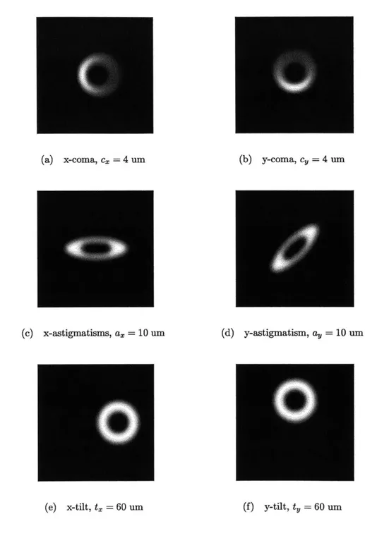
to evaluate Equation 2.9. The two main components of this computa-tion are the illuminated fraccomputa-tion f(zgdJ) and the inverse Hessian determinant, formulas for which can be found in Appendix A.

Six examples computed with this routine are given in Figure 3-1.

3.2

Fitting for Aberrations

The pairs of defocused images are fit using a Levenberg-Marquardt modified from

Numerical Recipes'

published version.

[]

In order to maximize speed, all of the derivatives are computed analytically using the formulas given in Appendix A. The fit contains fifteen total parameters: x-coma, y-coma, x-astigmatism, y-astigmatism, and the seeing radius are fit simultaneously using both images, while x-tilt, y-tilt, de-focus, total flux, and the background level are fit separately for each image in the pair. These five latter parameters are fit separately since, as the images in an out-of-focus pair are recorded on different detectors,

[ ] their tilts, total fluxes, and background

levels are likely different. Further, the defocus parameters are certainly different, as the detectors have been intentionally defocused to opposite sides of the focal plane.

The fit proceeds as follows:

1. Initial guesses are computed, as described in Section 3.3.

2. The Levenberg-Marquardt routine fits the images without fitting for the seeing radius.

3. The results of the previous fit are used as initial guesses for another Levenberg-Marquardt fit, this time with the-seeing radius included. This gives the final parameter values.

3.3

Initial Guesses

Initial guesses are generated for the fitting routine by first making the assumption that the coma and astigmatism parameters are zero. This is a reasonable assumption, as the maximum coma or astigmatism in the VISTA data is about 10 microns of wavefront error. Assuming only defocus and tilt are present, the aberrations can be estimated by iterating several image moments.

(b) y-coma, cy = 4 um

(c) x-astigmatisms, a. = 10 um (d) y-astigmatism, ay = 10 um

(e) x-tilt, tG = 60 um (f) y-tilt, ty = 60 um

Figure 3-1: Defocused images exhibiting d ~ 600 pm and exactly one of the other aberration parameters nonzero, with 1 arcsec blurring. The aberration parameters in these images are very large so as to clearly exhibit the types of distortion that they produce. In practice, the images analyzed by the fitting routine are much less distorted.

Suppose that we have estimates for the centroid of the image t2, and ty,n, the constant background value bn, and the radial size of the star An, we can then update these estimates by computing the following moments:

=yn~ (Y - ty,n) An,bn

2+1 = ((x - +x,n (y - ty,n

(I(x, y) - bn) (I - e_2n

bn+1~

~

(1 -

r/,n

where = X- ,,, = y-tV,, f = y 2 , and the moment (f (x, y))Ab is defined to be:

f

(x, y) (I(x, y) - b) e~(X2+Y2)/A2

(fxy))L~b =

E

(I(x, y) -b)

e-(X2+y2)/A2

This procedure is iterated until the change in the centroid values and the change in A is less than one pixel. Denoting the final values of this iteration with a subscript

f,

the initial guesses for defocus and total flux are set to be:

d

- ((X

-_

t,f)2 + (y - ty,f)2)Afbf

2

(R0

+

RL)

F

EZ(I(x,

y) - b) L

2

r ( - Ri)

where Rou and R., are the telescope pupil radii and L is the pixel width. Finally, the tilt and background values are simply set to be the final values of the above iteration, and the coma and astigmatism guesses are set to zero.

Chapter 4

Performance of the Fit Routine

4.1

Simulated Data

Producing Simulated Data

Simulated data was produced using the algorithm given in Section 3.1. This data exactly follows our model, and so there should be rapid convergence to the exact parameter values. The images measure 120 by 120 pixels and were produced using values for the pixel width, telescope radii and defocus parameter to match those of the VISTA low-order wavefront sensor, with a focal length of 12.072 m, inner and outer pupil radii of 0.8251 m and 1.85 m, respectively, and a defocus of about 280 microns of wavefront error, which corresponds to a 1.0 mm displacement from the focal plane. [.] Test images were generated with all possible combinations of zero and nonzero aberration parameters, with the values of the nonzero parameters chosen randomly from a predetermined range of values. The range of values for each aberration parameter was chosen empirically such that aberration values within the range produced roughly one or two pixels of distortion in the image, which is what is

Fits to Simulated Data

The fitting algorithm described in Section 3.2 was tested on simulated data, and the resulting fits converged rapidly and accurately. Initial guesses were generated using the routine in Section 3.3. After fitting a random sample of 500 simulated images, the longest convergence time was 20 iterations with an average of 14.53 iterations, which was about 520 ms, to convergence. The relative error between the randomly generated parameter values and the best fit values was on average 9.17- 10-7, and the worst-case fit value from the entire set of images had a relative error of 4.83 - 10-6.

4.2

VISTA Data

Fit Speed and Quality

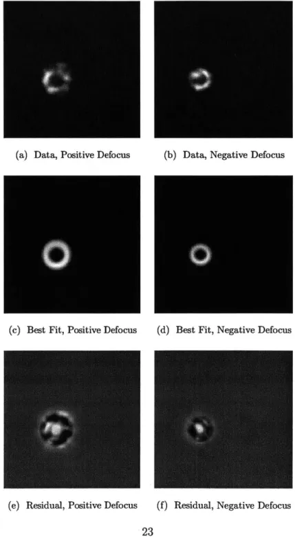
The fitting procedure was tested on 10 nights worth of VISTA wavefront-sensing data provided by the European Southern Observatory. 1 An example image from this dataset, as well as a best-fit image and residual, is given in Figure 4-1. This image and the resulting fit are very typical for the VISTA dataset. The fit routine has matched the large-scale size and shape of the image well, however there remains small-scale variations in the brightness internal to the star. This is likely due to the presence of unaccounted for higher-order terms in Equation 2.3. This causes a poor reduced chi-squared, Xrea = 8.57. The fit was rapid, however, converging in 26 total iterations, with 21 belonging to the initial unblurred fit and 5 to the blurred fit. These are typical values; over the entire dataset, the average reduced chi-squared was 5.73 and the average total number of iterations was 34. The best-fit values of the aberration parameters for one day (about 70 images) of the full ten day dataset (700 images) are given in the following plots, and any notable features of the data are discussed in the captions.

'We thank Thomas Szeifert, Andreas Kaufer and Magda Arnaboldi for arranging for the VISTA data to be recorded on our behalf.

Figure 4-1: An example fit to VISTA data. While the large-scale fit matches the im-ages overall shape and size well, there are clear higher-order variations in the residual that the model does not account for. Also, note the very high intensity in the "hole" of the annulus on the residual image; the cause of this is currently unknown. This drives up the Xed value to 8.6. The Xed was computed using the square root of the photon count as the error. For this fit, the number of iterations before convergence was 26. The fit was taken over the entire 120x120 image, all of which is pictured.

(a) Data, Positive Defocus (b) Data, Negative Defocus

(c) Best Fit, Positive Defocus (d) Best Fit, Negative Defocus

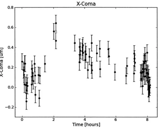
X-Coma

4

Time [hours]

Figure 4-2: This This time period bars are taken to

is the best fit x-coma, plotted over time for 1 night of observing. correspond to about t = 4.6 days on the 10-day plots. The error be the median discrepancy taken from Table 4.2.

0.8 0.6 0.4

-E

E

0

U

>k

0.2 -

0.01-I

I

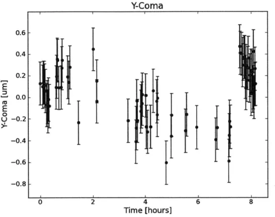
-0.2 V 0 2 6 8

Y-Coma

0.6 0.4 0.2-0.0

E

U -0.2 ---0.4 -0.6--0.8 0 2 4 6 8

Time [hours]

Figure 4-3: This is the best fit y-coma, plotted over time for 1 night of observing.

This time period correspond to about t

=

4.6 days on the 10-day plots. The error

bars are taken to be the median discrepancy taken from Table 4.2.

0.4 0.2

[

0.0-E

. -

x

V) Ifl

x

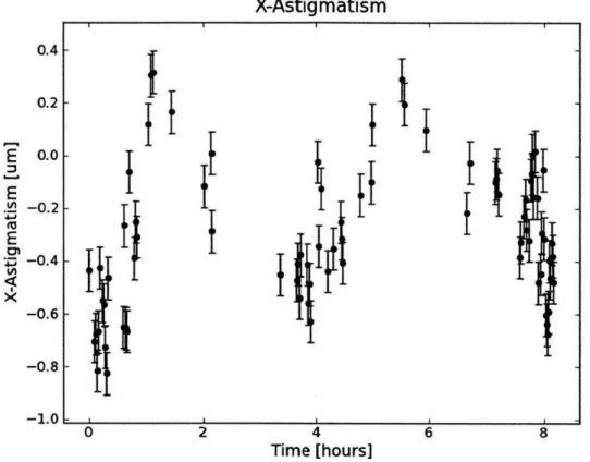
-0.2 -0.4 -0.6--0.8 -1.0

X-Astigmatism

0 2 4

Time [hours]

6 8

Figure 4-4: This is the best fit x-astigmatism, plotted over time for 1 night of ob-serving. This time period correspond to about t = 4.6 days on the 10-day plots. The error bars are taken to be the median discrepancy taken from Table 4.2.

E

E

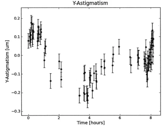
0.2 0.1 0.0 -0.1 -0.2 -0.3

Y-Astigmatism

'k-0 2 4

Time

[hours]

6 8

Figure 4-5: This is the best fit y-astigmatism, plotted over time for 1 night of

ob-serving. This time period correspond to about t

=

4.6 days on the 10-day plots. The

error bars are taken to be the median discrepancy taken from Table 4.2.

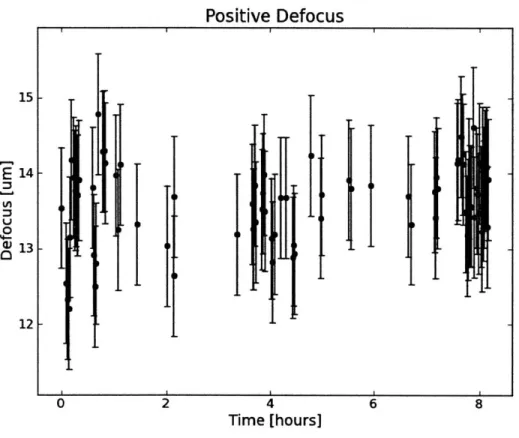
15 k E 14 LA 13 12

Positive Defocus

0 2 4 Time [hours] 6 8

Figure 4-6: This is the best fit defocus for the pre-focal image, plotted over time for 1 night of observing. This time period correspond to about t = 4.6 days on the 10-day plots. The error bars are taken to be the median discrepancy taken from Table 4.2.

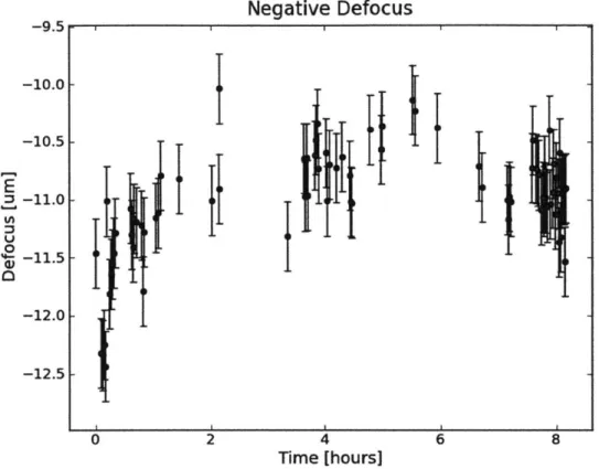
Negative Defocus

2 4

Time [hours]

Figure 4-7: This is the best fit defocus for the post-focal image, plotted over time for

1 night of observing. This time period correspond to about t

=

4.6 days on the 10-day

plots. The error bars are taken to be the median discrepancy taken from Table

4.2.

-9.5-. -10.0--10.5 F 11.0

11.5-E

U 0 -) --12.0 1 -12.5 -0 6 8

1500 1000 -500 I-0 -500 1000 --1500 --2000

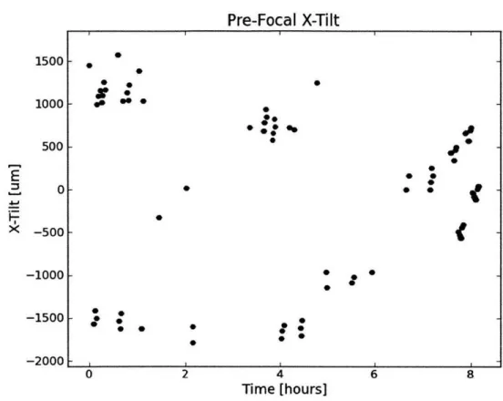
Pre-Focal X-Tilt

0 2 4

Time

[hours]

6 8

Figure 4-8: This is the best fit x-tilt for the pre-focal image, plotted over time for 1 night of observing. This time period correspond to about t = 4.6 days on the 10-day plots. The error bars are taken to be the median discrepancy taken from Table 4.2. Note the clumping of the data; this corresponds to the 6 dithers used by VISTA for a given pointing.

[

E

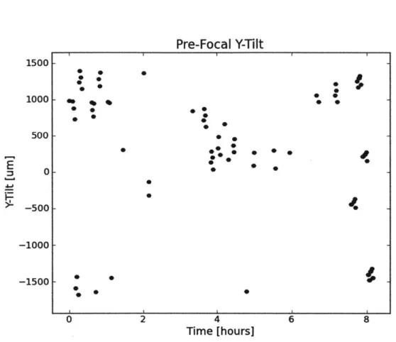
0 e ** ** * 0 0@e * 0 * 0* * * 0 . e e

1500 1000 1- 500-0 -500 --1000 --1500 -0

Pre-Focal Y-Tilt

2 4

Time [hours]

6 8

Figure 4-9: This is the best fit y-tilt for the pre-focal image, plotted over time for 1

night of observing. This time period correspond to about t

=

4.6 days on the 10-day

plots. The error bars are taken to be the median discrepancy taken from Table 4.2.

Note the clumping of the data; this corresponds to the 6 dithers used by VISTA for

a given pointing.

_[

]

1

E

* *, . 0e . * 0 0 *

Fit Errors

Since the X 2 values for these fits are poor, the error estimates produced by the

fit routine are not reliable and underestimate the error by a factor of 4 to 8, when compared to the errors given in Table 4.2. Instead, I will estimate the error by looking at the variation in the fit values extracted from very similar images. The VISTA data consists of 120x120 pixel pieces taken from a 2Kx2K detector, and the header includes the pixel coordinates of the lower-left pixel of the 120x120 image. From the dataset, I selected images for which this pixel was located in exactly the same spot on the full detector, and further, from this set I selected all of the pairs of images that were observed consecutively. Generally, these consecutive observations were separated by an interval of about 50 seconds, and had an integration time of 25.0 seconds. Since these images were taken at nearly the same time, and the star did not change positions on the detector between the images, it is reasonable to assume that the star in both images is the same, and that the telescope did not move appreciably between the images. Thus, the difference in aberrations should be very small and any discrepancy between the fitted aberration values for these images can be attributed to the fitting routine. The maximum and median of the magnitude of this discrepancy, taken over all such pairs of images, is reported in Table 4.2 and Table 4.2. The median values can be taken to give a typical uncertainty and the maximum values give the worst-case uncertainty.

Another way to estimate the fitting errors is to consider the variation in time of combinations of parameters that should be constant. The defocus parameter for each image in a pair consists of a component due to the alignment state of the telescope and another component due to the position of the wavefront sensor. The wavefront sensor components for the VISTA images should be nearly equal in magnitude but of opposite sign and it should remain fixed in time, whereas the telescope components will be equal for each image and varying with time. Thus, the difference of these two values will be constant. Any variation in this quantity, which is plotted in Figure 4.2, should be attributable to the uncertainties of our measurement. From the figure, it is

Table 4.1: This table gives statistics of the magnitudes of the discrepancies of fit values extracted from very similar images. Aberration units are in microns of wavefront error, flux and background are given in photon counts, and the seeing diameter is in arc seconds. The median value gives a typical error bound, and the maximum values an upper error bound. Note the very small discrepancies for the total flux parameters, seeing diameters, and background level (the absolute scale of the background is about 750 photon counts), which affirms that we are looking at the same star in both images. Also, the values for y-coma are about 3 times larger than the other coma and astigmatism parameters.

warns that the reported error astigmatism parameters differ understood.

The cause of this is not yet understood, however it for x-coma is likely too small. Finally, note that the by a factor of 2; the cause of this is also not currently

Parameter Minimum Median Maximum Coma x 0.0009207 0.07955 0.523 Coma y 0.001261 0.179 1.413 Astig x 0.01432 0.08325 0.4041 Astig y 0.002016 0.04104 0.1978 Seeing Diameter 0.00669 0.1539 1.37 Tilt x+ 0.007977 0.6695 4.725 Tilt y+ 0.07267 0.5656 2.57 Defocus+ 0.0102 0.2826 2.286

Flux+ 2.487e-08 4.168e-07 2.865e-06 Bkgnd+ 0.0494 4.688 43.53

Tilt x- 0.02365 0.8693 5.39 Tilt y- 0.01017 0.7276 2.593 Defocus- 0.02416 - 0.2809 2.286

Flux- 2.723e-08 4.176e-07 2.147e-06 Bkgnd- 0.2406 5.331 48.72

clear that the scatter is consistent with the uncertainty estimates given above, which lends more credibility to the estimates given in Table 4.2. The same reasoning applies to the x and y components of tilt, whose difference is plotted in Figures 4.2 and 4.2. These plots are less consistent than the defocus difference, but not alarming so.

Difference in Defocus of the Pre and Post Focal Images

28 C 0 27 -26 -25 -24 -23 -0 2 4 Time [days] 6 8

Figure 4-10: A plot of the defocus difference, which in principle should be constant in time. I have plotted this data with error bars set the median discrepancy taken from Table 4.2, in order to show that the scatter over time in the defocus difference is consistent with the median errors from Table 4.2. While there are a few obvious outliers, the data is clearly consistent with a constant function. The units of defocus are given in microns of wavefront error.

Table 4.2: These are the same results as in Table 4.2,

errors in the Zernike coefficients using the conversions in are given in microns of wavefront error.

but have been converted to Section 2.5. All of the values

Zernike Number Minimum Median Maximum

1 0.04304 0.7554 2.675 2 0.07267 0.6947 2.574 3 0.02416 0.2809 2.286 4 0.01432 0.08325 0.4041 5 0.002016 0.04104 0.1978 6 0.0003069 0.02652 0.1743 7 0.0004204 0.05968 0.4709

Difference in X-Tilt of the Pre and Post Focal Images

-I

0 2 4

Time

[days]

6 8

Figure 4-11: A plot of the x-tilt difference, which in principle should be constant in time. I have plotted this data with error bars set the median discrepancy taken from Table 4.2. While the the data is not rigorously consistent with a constant function, it is very close. The units of defocus are given in microns of wavefront error.

4086[ C 4084 4082 4080 4078 4076

0)" E U 5 4 3 2 1 0 -1 -2 -3

Difference in Y-Tilt of the Pre and Post Focal Images

* jiit

0 2 4

Time [days]

6 8

Figure 4-12: A plot of the y-tilt difference, which in principle should be constant in time. I have plotted this data with error bars set the median discrepancy taken from Table 4.2. As with the x-tilt difference (Figure 4.2), the the data is not rigorously consistent with a constant, it is very close The units of defocus are given in microns of wavefront error.

Chapter 5

Conclusion

In this work I have described a new algorithm for extracting measurements of optical aberrations from a pair of oppositely defocused images. The model was verified using simulated data, and also applied with some success to VISTA data. The VISTA fits were able to fit the data rapidly and provided a consistent estimate of the fitting errors, at a reasonable scale of 0.08 um for coma, 0.08 um for astigmatism, 0.9 um for tilt, and 0.3 um for defocus. However, but the model is also clearly unable to account for higher-order aberrations, and probably other effects as well, that are present in the VISTA data. As such, there is certainly room for improvement, and expanding the model from its present state to account for at least some subset of these currently un-modeled effects will likely result in a much more accurate determination of the

Appendix A

Formulas

In this section I will give the exact formulas that are used in the software implementa-tions of the algorithms given in Chapter 3. In most cases, these results follow directly from the definitions in Chapter 2 and some tedious but straight-forward computation, in which case I will simply report the final result. However, there is some subtlety in a few of these computations, and for those cases I provide a derivation.

A.1

Illuminated Fraction

To find the illuminated fraction of a defocus-only pixel, we need to solve the following problem: Given a square pixel of length 1 centered on the point (xdf, yg), what fraction

#

of its area is enclosed by a circle of radius R centered on the origin? The illuminated fraction

f

is given by the enclosed fraction $(zdf, R) as:

{$(,

2dRou) |rg - 2dRoti <

f (Z

i)

= 1 - #(zg, 2dRin) |rd - 2dRin| < ' (A.1)

0 Otherwise

where rdf = zf yj. In this formula, I have assumed that the three cases are mutually exclusive, which will be true in any realistic telescope.

frac-tion of the pixel will be invariant if we reflect the pixel across any line through the origin. Thus, I will restrict attention to pixels with coordinates 0 xdf 5 ydf, which significantly reduces the number of special cases that we need to consider. Second, in any realistic telescope we will have that R

>

1, and so I will approximate the circle by its tangent line in the vicinity of (xv, ydf). The tangent is given by

y

= - x + L

R

(A.2)

Ydf Ydf

There are five special cases to consider, two of which are trivial:

1. The pixel is inside the circle:

4

= 1. 2. The pixel is outside the circle:

4

= 0.

3. The circle crosses the left side and the bottom of the pixel. 4. The circle crosses both the left and right sides of the pixel.

5. The circle crosses the top and right side of the pixel.

We need a computational way of differentiating between these cases. To do this, consider the quantity y, which gives the y-coordinate at which the tangent line intersects the vertical line coincident with the right edge of the pixel:

y,= ±(xg + 1/2) + R (A.3)

Ydf Ydf

This expression can be made easier to work with by defining a dimensionless quantity -y, which gives the distance between the top of the pixel and the intersection point y, in units of the pixel length:

1

(

7 Ydf - Y,) (A.4)

Then the above conditions become:

2. The pixel is outside the circle: 7 > 1

+

xdf/Ydf

3. The circle crosses the left side and the bottom of the pixel: 1 < -Y < 1 +xdf/Ydf

4. The circle crosses both the left and right sides of the pixel: xdf/Ydf < 7 < 1

5. The circle crosses the top and right side of the pixel: 0 <7 < xdf/ydf

All that remains is to calculate the fractional area of the pixel that lies below the tangent line. This is straightforward geometry, and the results are:

1. The pixel is inside the circle:

2. The pixel is outside the circle:

# =0

3. The circle crosses the left side and the bottom of the pixel:

)2

4. The circle crosses both the left and right sides of the pixel:

S= + Xdf 2yg

5. The circle crosses the top and right side of the pixel:

1 Ydf

-#=1- -- 72

A.2

Derivative of Illuminated Fraction

Directly from Equation A.1, the derivative of the illuminated fraction with respect to some parameter a is:

df

Ird -

2dRot <

df d 2

da = O

Irr

- 2dRin| <

0 Otherwise

The enclosed fraction

#

is a function of three variables: the defocus-only pixel coordinates xdf and ydg, and the radius of the circle. The derivative with respect to

a is therefore:

do_ _ o aqxdf &ao ftdf co~7 MR(A

-+ -+- (A.5)

da Ox4 aa 0ydf aa

OR Oa

The defocus-only position partials are computed in Section A.5. The three partial derivatives of

p

appearing in Equation A.5 are given by simply differentiating the expressions for

p

derived in Section A. 1. These are most clearly expressed as functions of xd, yg, and partial derivatives of the parameter -y with respect to defocus-only-positions. This gives the formulas:

1. The pixel is inside the circle:

= -_- - -0

oxdf -ydf OR

Oa

2. The pixel is outside the circle:

--

d

= -- =-- =0

3. The circle crosses the left side and the bottom of the pixel: ___ = _{1 1} 1 i-I

axdf

2 ydf

o

- Xdf1 9 Ydf 2y 2 0 R 5a,d 1 - ( x 12 x - 1) (7-1)df Xdf

4. The circle crosses both the left and right sides of the pixel:

&4 O9Xdf o OYdf 005

OR

OpR Ra

_ 1 fry 2_{ydf Oxgf}

2yg 2yf 2y OYdf rdf R -

ocnd

_d

5. The circle crosses the top and right side of the pixel:

OXdf OYdf

Ob OR

fry

1

9 Xdf Ydf .ry. . 1 aYdf _df = Ydf Xdf

(

fY aXdf Ydf (ry

Kd

'9

Ydf±

rdf R

-d ond

1

₊₍

_x

₍₂

]

R

2

1

rg) S)2 2y ) 1

1

(2

rdfR) dxdf (i)df)

ary

Xdf ) Ydf where:

A.3

Hessian Matrix

The Hessian matrix H is the Jacobian of the transformation in Equation 2.7. This is given by:

H ( 2d C Xdf + = Y Ydf Ax40y d ±1 +1 jXdf±+ Cxq+ 21yf yg + I xd +±Ydf + ±Xd5 + Vys - + 1

It is useful to have an expression for det H', for use in computing H-' and for computing the brightness. As a polynomial in the pupil position, it is given by:

1

3Cx

- C2 3C2 _ C2

2CxC,

det H 4d2 _{df + 4d}2 _{Yf+ Xdf Ydf}

1 'F

A ,

CA

l 1

A,

CA,]

1 d dJ

A.4

Derivative of the Brightness

In order to use this model to rapidly fit for the aberration parameters of an image, it is necessary to have an analytic expression for the gradient of a given pixel's brightness with respect to the set of aberration parameters and the total flux

F.

The brightness of a pixel is given by Equation 2.9:

F

1

Ix(z2)- Xf ₎₊

4d2 _det(H(2))|

Differentiating this with respect to a parameter a gives four terms:

I b F p l s g1

-. =f - -q - +b

Ba 4d2| det(H)I Ia 4d2 Ba det(H)|

F 1 1 1

The determinant derivative is:

a

(

iI

_{a_(I|det}

_(H))

I

1 det (H)

(det(H))

Idet(H)12 det(H) a(e

_ 1

Idet(H)|

'Tr H = -etH det(H) Tr H-1 H

I|det (H)|12 det(H)

a

_ 1 _H = 1 Tr H-1 a

Idet(H)|

da and so the full brightness derivative is:

aI

F 1

Of

F 1 H1

H\

a 4d2 Idet(H)Ia 4d2|det

Tr

H

f

(A.6)

F 1 1 1

2d3

I

det(H)|

I

det(H) I

1 1

f

/

H

2

det(H

L

F

- Tr H-1 F

f

- , +6,FJ + Ea,bcFf

4d2 de(H 18 \ a} dF ± I

Now, if

f

is zero then the last two terms vanish. The term af/Ba will also vanish (see Equation A.2). This makes sense, as

f

= 0 corresponds to an unilluminated background pixel. In addition, F represents the total flux through the pupil, and so for any image it must be nonzero. Since we will therefore only evaluate the above expression when

f

0 0 and F =, 0, it does no harm to factor out a factor of

f

and F to give the final formula:

0I

rH

1__ 2 1 ]

a

= I -Tr

+

+ 2,

-H-1 + a,b (A.7)

This is the form of the derivative that will be used by the fitting routine. Note that while there are five terms, it is rarely necessary to evaluate all of them. Of the four bracketed terms, the first encodes the change in brightness of an interior pixel and is always nonzero for illuminated pixels. The second accounts for the large change in brightness that occurs near the edge of the image due to the shifting boundaries of the illuminated region, and it is only nonzero for border pixels. The third and fourth

terms include the overall change in brightness that occurs when the defocus or total flux is varied, respectively. These terms come from the fact that the brightness of the defocus-only image changes when the total flux or defocus is varied.

A.5

Derivative of the Defocus-Only Position

To compute the derivative of the brightness of a pixel with respect to an aberration parameter, we need to know how the defocus-only position changes if we fix the image position and vary an aberration parameter. The defocus-only position and the image position are related by Equation 2.7. I will rewrite this in the more compact form:

Xi= V fW(zd) (A.8)

Since the image coordinates x and yi are fixed, differentiating with respect to an aberration parameter a gives zero on the left-hand side. Applying the chain rule to the right-hand side gives:

d

0 = - [V+ W(z)} (A.9)

= [VdW(')] ±

2

-Jdf (VdfW(zd))

(A.10)

where Jd(f('d)) denotes the Jacobian matrix of

f(Zg)

with respect to

4.

But,

Jdf (VdfW(zgd))

is just the Hessian

H(zg),

so:

0= [VdfW(g)]+ -H(zg)

Thus the derivative of the defocus-only position with respect to a is:

taxdf

a

d -1()

Let d = (VdW(zdf)]. This vector is given by:

xf5 ±t - y25 + IXdfYdf + 5Xdf

yd + x5 ± jy5 + 2XdfYdf + Xd

Working this out, the defocus-only position derivative is:

d5df =

_g

_{- H -1(zaf} + Ay5+T ± Ydf Tx -d Ydf ±

Ti']

where: 3 x2 _1 Y2 42df 4T ydf 1 -jxdfyd5 -X yg3 -$72 -f

Nd

Ydf Xdf d

(

1df)

(

d!

d Xdf) (0i 0

-1)

24y + y Xdfyd +^ x + y Ydf

+(

±fx :+±

Yf

+

Xdf Ydf+^Xdf+ydf) if a = Cx if a _{= C,} if a=A, if a=AY if a=Tx if a =Ty if a=d

A.6

Derivative of the Hessian

The Hessian matrix is:

T ldfXdf + -- y-Ydf 2d2 A, d CV Xdf + C' 2d2 2d2 Ydf + I d2CY X df + 2 d-z2C -Ydf + 'd CT + 3Cy AT, + 2d Xdf 2d2 Ydf

Differentiating this is straightforward. Note that the derivative matrix will contain some terms that will be present for any differentiation parameter a and some terms that depend on a. It is useful to separate these two pieces, as the term that is constant in a only needs to be evaluated once per pixel, and so I express the derivative as:

dH C + C dydf

H

22 da 2 da da C dxdf C dy_ 2 da 2 da C dxd_ ±CT dYdf 2 da 2d2 da C dxad 3C da / 22 da 2 da)

1 1 Qxdf MXdf 1 3

(

pyXdf

gYdf/

if a= Ay

if a E{TX7,Ty,

(- Xd -- Ydf -~ -yXdf ~ :Ydf - 4 C 3C A -- Xdf - 7KYdf ± t where: 3

(2Xdf

1 =2d Ydf 1 27IYdf 1 2Xdf if a=C,

if a= A

d

o

-1

r/a = < 0 1_d o 0

0

0

0

0)

if a=d

Appendix B

Software

B.1

Fitting Program

The program abr_fit-image, written in C++, will sequentially fit any number of .FITS whose filenames are passed as command-line arguments. The results of the fit will be printed to stdout in the following order:

1. filename of target .FITS file

2. the initial guesses used by the routine

3. best fit parameter values

4. covariance matrix entires, starting with the upper left entry and working down to the lower right entry

5. total number of iterations before convergence 6. final chi-squared value

7. total degrees of freedom

8. final value of the Levenberg-Marquardt damping factor

The convention for ordering the parameters is: c2, cy, ax, ay, s, t2+, ty+, d+, F+, b+, t2-, ty -, d-, F-, b-, where the

+

and - symbols indicate a parameter that is