Analysis and control of contagion processes on networks

Analysis and Control of Contagion Processes on

Networks

by

Kimon Drakopoulos

Submitted to the Department of Electrical Engineering and Computer

Science

in partial fulfillment of the requirements for the degree of

Doctor of Philosophy in Computer Science and Engineering

at the C

MASSACHUSETTS INSTITUTE OF TECHNOLOGY

F

June 2016

_L

Massachusetts Institute of Technology 2016. All rights reserved.

Author ..

E S I$ TUTE IFTECHNOLGY

UL 12 2016

IBRARIES

ARHIVES

Signature redacted

Department of Electrical Engineering and Computer Science

A

May 20, 2016

Certified by...

Signature redacted

...

Asuman 6zdaglar

Professor

Al ---- A AT-kesis

Supervisor

Certified by...

Signature

redacted...

I

Accepted by ...

A1

jonn N. Tsitsiklis

Professor

Thesis Supervisor

Signature redacted

_....

Les1Q W. Kolodziejski

Professor

Chair, Department Committee on Graduate Students

Analysis and Control of Contagion Processes on Networks

by

Kimon Drakopoulos

Submitted to the Department of Electrical Engineering and Computer Science on May 20, 2016, in partial fulfillment of the

requirements for the degree of

Doctor of Philosophy in Computer Science and Engineering

Abstract

We consider the propagation of a contagion process ("epidemic") on a network and study the problem of dynamically allocating a fixed curing budget to the nodes of the graph, at each time instant. We provide a dynamic policy for the rapid containment of a contagion process modeled as an SIS epidemic on a bounded degree undirected graph with n nodes. We show that if the budget r of curing resources available at each time is Q(W), where

W is the CutWidth of the graph, and also of order Q(log n), then the expected time until the extinction of the epidemic is of order O(n/r), which is within a constant factor from optimal, as well as sublinear in the number of nodes. Furthermore, if the CutWidth increases sublinearly with n, a sublinear expected time to extinction is possible with only a sublinearly increasing budget r.

In contrast, we provide a lower bound on the expected time to extinction under any such dynamic allocation policy, for bounded degree graphs, in terms of a combinatorial quantity that we call the resistance of the set of initially infected nodes, the available budget, and the number of nodes n. Specifically, we consider the case of bounded degree graphs, with the resistance growing linearly in n. We show that if the curing budget is less than a certain multiple of the resistance, then the expected time to extinction grows exponentially with

n. As a corollary, if all nodes are initially infected and the CutWidth of the graph grows

linearly in n, while the curing budget is less than a certain multiple of the CutWidth, then the expected time to extinction grows exponentially in n.

The combination of these two results establishes a fairly sharp phase transition on the expected time to extinction (sublinear versus exponential) based on the relation between the CutWidth and the curing budget.

Finally, in the empirical part of the thesis, we analyze data on the evolution and prop-agation of influenza across the United States and discover that compartmental epidemic models enriched with environment dependent terms have fair prediction accuracy, and that the effect of inter-state traveling is negligible compared to the effect of intra-state contacts. Thesis Supervisor: Asuman Ozdaglar

Title: Professor

Thesis Supervisor: John N. Tsitsiklis Title: Professor

Acknowledgments

In the clearing stands a boxer, and a fighter by his trade, And he carries the reminders of every glove that laid him down And cut him till he cried out, in his anger and his shame,

"I am leaving, I am leaving." But the fighter still remains

Paul Simon

On the first year of my PhD, I met with an alumnus from the Laboratory for

Information and Decision Systems (LIDS) who argued that his years at MIT had

been the best years of his life. At that point, that statement sounded absurd. Seven years after this conversation, I can now relate to his experience. Being a person who seeks adventure, I admit that the past years have been the most challenging, life-changing and exciting adventure so far. There are several people who made this adventure more didactic, more enlightening and definitely more enjoyable.

First and foremost, I would like to express my gratitude to my phenomenal ad-visors, Asu Ozdaglar and John Tsitsiklis as well as my committee member Daron

Acemoglu. Their guidance throughout my graduate studies made me a better

re-searcher but most importantly a better person. I will always be indebted to them for

their support, their ideas and admittedly their patience.

Asu, I do not have enough words to describe how much I owe you. Thank you

for nurturing me since my first day at MIT, thank you for exposing me to exciting

problems and research directions, thank you for teaching me how to look at the

big picture of things, thank you for your enthusiasm, the bright outlook and the

"pep talks" in your office that was always open regardless of your busy schedule and countless responsibilities.

John, you have been one of the most influential people in my life. Thank you for introducing me to the magical powers of simplicity, thank you teaching me how

to structure my thoughts and my approach to problems. I should even thank you

(and I never thought I would say this) for your comments, edits and the suspense of sending you drafts of my work. Interacting with you has been invaluable both for my

academic and my personal maturation.

Daron, there is no need to praise your academic ingenuity or your incredible mentorship, as at this point these are widely recognized. I should thank you, though, for finding the time for me to discuss research problems and life decisions.

During my graduate studies at MIT, I was privileged to serve as a TA for John Tsitsiklis, Patrick Jaillet, Asu Ozdaglar, Polina Goland, Itai Ashlagi and as an instruc-tor for the Leaders for Global Operations. I would like to thank both the instrucinstruc-tors and the students for helping me mature as a lecturer and for introducing me to one of the most rewarding aspects of academic life, teaching.

Moreover, I would like to extend my gratitude to the LIDS staff, and in particular Roxana Hernandez, Jennifer Donovan, Lynne Dell, Petra Aliberti and Brian Jones for their help with various administrative tasks as well as for letting me in my office on an almost daily basis. Furthermore, I would like to thank the funding sources of this thesis: Draper Laboratories and the Army Research Office's Multidisciplinary University Research Initiative .

I was extremely fortunate to be part of the stimulating and energetic LIDS

com-munity and in particular the Optimization and Network Game Theory, and Systems, Networks and Decisions groups. I would like to thank all members of LIDS and in particular Kostas Bimpikis, Ozan Candogan, Alireza Salehi, Mihalis Markakis, Ali Makhdoumi, Elie Adam, Spyros Zoumpoulis, Paul Njoroge, Ermin Wei, Mert Giir-biizbalaban for being incredible collaborators, friends and coffee-drinking partners.

The past several years would not have been as enjoyable or even bearable if it was not for the company of my dear friends, Ampelale, the Greeks of Boston, and in particular Georgios Angelopoulos with whom we started and ended the PhD journey, my dear friend and roommate Dimitris Chatzigeorgiou, and Yola Katsargyri who was a supporting companion during the emotionally challenging and stressful last PhD years.

Concluding, throughout my life and my PhD studies in particular, I have been spoiled by the support, kindness and generosity of two extraordinary individuals. Mom and Dad, this thesis is dedicated to you.

Contents

1 Introduction

1.1 Problem and Motivation ...

1.2 Related literature . . . .

1.3 Simple examples . . . .

1.3.1 Example I: the line graph . . . .

1.3.2 Example II: the two dimensional grid 1.4 Contributions of this thesis . . . .

1.5 Structure of the thesis . . . . 2 Model and Graph Theoretic Preliminaries

2.1 Controlled Contact Process . . . . 2.2 Main Problem . . . .

2.3 Discussion on the Model . . . . 2.4 Graph Theoretic Preliminaries . . . . 2.4.1 Notation and Terminology. . . . . 2.4.2 Cuts, CutWidth, and Resistance. . . 2.4.3 Properties of the resistance. . . . . . 2.4.4 Relating cuts to the resistance. . . . 2.4.5 Properties of the impedance . . . . . 2.4.6 Resistance and Impedance . . . .

3 An Efficient and Optimal Curing Policy 3.1 Description of the CURE policy . . . .

19 . . . . 19 . . . . 22 . . . . 24 . . . . 25 . . . . 25 . . . . 26 . . . . 28 29 . . . . 29 . . . . 31 . . . . 32 . . . . 33 . . . . 34 . . . . 35 . . . . 37 . . . . 39 . . . . 40 . . . . 41 49 49

3.2 Performance Analysis . . . . 51

3.2.1 Segment analysis . . . . 52

3.3 Corollaries and near-optimality of the CURE policy . . . . 55

3.4 Performance of the CURE Policy under arbitrary initial infections . . 57

3.5 Simulation Results . . . . 60

3.6 Discussion and Conclusions . . . . 63

4 A lower bound for graphs with very large CutWidth: a special case 65 4.1 More properties of optimal crusades and implications . . . . 67

4.1.1 Characterization of optimal crusades and some implications . 69 4.2 Exponential Lower Bound . . . . 74

5 A lower bound for graphs with linear CutWidth: the general case 79 5.1 The main result and the core of its proof . . . . 79

5.2 Proof of Lemma 15 . . . . 82

5.3 Proof of Lemma 17 . . . . 84

5.4 Proof of Lemma 16 . . . . 86

5.4.1 Decomposing the event of interest . . . . 88

5.4.2 Bounding P(Bi) . . . . 89

5.4.3 Completing the proof of Lemma 16. . . . . 93

5.5 Conclusions . . . . 93

6 Summary of Theoretical Results and Open Questions 95 6.1 Case I: All nodes initially infected . . . . 95

6.2 Case II: Some nodes initially infected . . . . 97

6.3 Conclusions of the theoretical part of the thesis . . . . 98

7 Modeling Infectious Diseases: Influenza in the United States 101 7.1 Networked Compartmental Models . . . . 102

7.2 Connections between Compartmental and Stochastic models . . . . . 105

7.3 D ata . . . . 107

7.5 Estim ation . . . . 117

7.5.1 Identifiability of network effect z . . . . 117

7.5.2 Learning dependence on humidity and mixing rates . . . . 120

7.6 A preliminary approach to identifying network effects . . . . 129

7.7 Summary and Conclusions . . . . 131

List of Figures

1-1 An efficient dynamic curing policy for the line graph would allocate all curing resources to the right-most infected node. . . . . 25

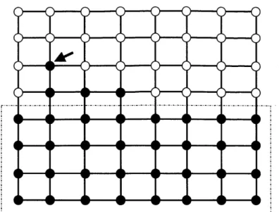
1-2 An efficient dynamic curing policy for the grid graph would allocate all curing resources to the top-right infected node. . . . . 26

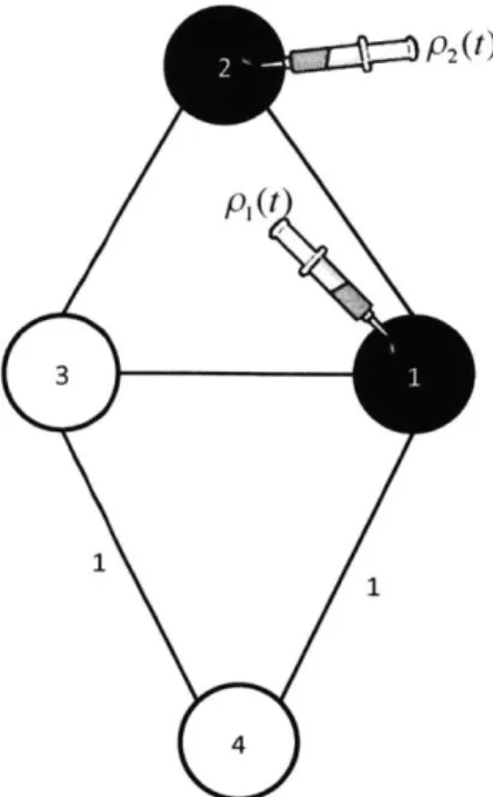
2-1 The controlled contact process: each node can be either infected (black) or healthy (white). Infected nodes infect their healthy neighbors ac-cording to a Poisson process with rate 1. Infected nodes get cured according to a Poisson process with rate pv(t) that is determined by the network controller. . . . . 30

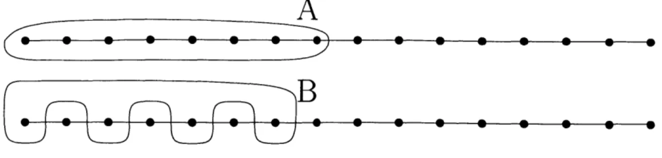
2-2 A line graph with n nodes (n is a multiple of 4). Bag A consists of

n/2 nodes. Bag B consists of the odd numbered n/4 nodes of bag A.

The impedance and the resistance of bag A coincide and are equal to

1. However, the impedance of bag B is equal to n/2 - 1 while the resistance of bag B is equal to 1. . . . . 42

3-1 Performance of three policies on a star graph with 51 nodes. . . . . . 62 3-2 Performance of three policies on a 5 x 10 mesh graph. . . . . 62

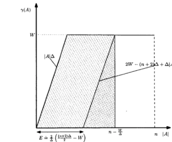
4-1 Admissible region for the pair (-y(A),I A). If -y(A) < W, Lemma 11 im-plies that (-y(A), AI) belongs to the parallelogram shown in the figure. On the other hand, there is no restriction on the size JAI of bags with y(A) = W, and so the admissible region also includes the horizontal

5-1 Case 1: In the first case, c(It) remains at least -y/4 throughout the

interval [0, T]. Moreover, since the resistance drops from -y to y/2, at least -y/2 recoveries must occur. Case 2: In the second case, c(It) drops below -y/4. The last time that it does so (time T'), the resistance is above y/2 and needs to drop to a value below y/2. Therefore, c(It) needs to grow above (roughly) -y/2. In principle, this increase may happen through infections and not only through recoveries. This is why we define the auxiliary process

E8,

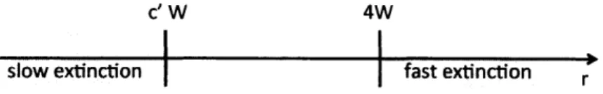
whose cut also needs to increase to 'y/ 2 _{but can only increase through recoveries, implying that at least}

(roughly) 7/4A recoveries occur. . . . . 87 6-1 Slow vs. fast extinction for graphs with large CutWidth. The ratio

of the curing resources to the CutWidth is the key factor that distin-guishes between slow and fast extinction. . . . . 96 6-2 Slow vs. fast extinction for graphs with small CutWidth. If the curing

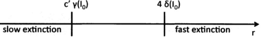
budget is larger than the CutWidth of the graph, then fast extinc-tion is achieved. Otherwise, we conjecture that fast extincextinc-tion is not achievable. . . . . 97 6-3 If the curing budget is larger than the the impedance of the set of

initial infections, then fast extinction is achieved. On the other hand, fast extinction is achievable if the curing budget is smaller than the resistance of the set of initial infections. . . . . 98 7-1 The metapopulation model for the United States . . . . 107 7-2 Number of influenza related infections in Arizona for the 2008-2009

season. The single peaked shape of the time series is typical in the dataset. . . . .111

7-3 Relation between number of infections and absolute humidity of the

preceding week in Arizona, for the 2008-2009 season. We plotted the logarithm of each quantity for illustration purposes. The slope for this case is equal to -0.37. . . . 113

7-4 Travel intensities (normalized) as calculated using data from the Na-tional Household Travel Survey (NHTS). . . . . 115 7-5 Normalized infections within the state of Colorado as well as traveling

infections into the state for the season 2011-2012. Identifying network effect z is impossible due to collinearity. . . . . 118 7-6 Normalized infections within the state of Kentucky as well as traveling

infections into the state for the season 2011-2012. Identifying network effect z possible due to orthogonality. . . . . 119 7-7 Orthogonality between the vectors of in-state infections and traveling

infections, for each state i e

{1,

50} and each season s E {1, ... , 8}. . 120

7-8 In blue: season-state pairs where identification of network effect is

im-possible. In yellow: season-state pairs where identification of network effect is possible. . . . . 121

7-9 Non linear regression: The fitted model is accurate. Prediction using the estimated model is not. . . . . 122

7-10 One step vs Long term prediction . . . . 123 7-11 Different shapes of logistic functions . . . 127 7-12 Example of fit: simulated vs. real infection time series for a

state-season pair in the training set T. . . . 128 7-13 Dependence of effective contact rate on absolute humidity for different

seasons... ... .... ... .. .. .. . . 129

7-14 Example of prediction: predicted vs. real infection time series for a state-season pair in the validation set T. Prediction error for this case is 0.503, which is the smallest prediction error achieved within the whole validation set. . . . . 130

7-15 Example of prediction: predicted vs. real infection time series for a

state-season pair in the validation set

T.

Prediction error for this case is 1.471, which is one of the largest prediction errors achieved within the whole validation set. For this particular state-season pair, and for those with large prediction error, the absolute humidity does not seem to correlate negatively with the increase of the number of infections. Such pairs are an exception both in the training and the validation set. 130

List of Tables

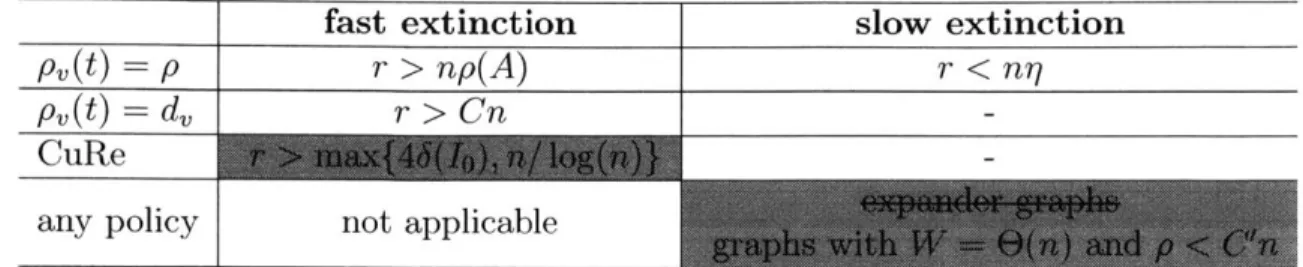
1.1 Existing Results: Conditions for fast and slow extinction under differ-ent curing policies, assuming all nodes initially infected. . . . . 24

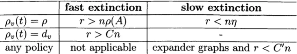
6.1 Existing and New Results: Conditions for fast and slow extinction

under different curing policies, assuming all nodes initially infected. . 97 7.1 Results of linear regression to identify network effects. . . . . 131

Chapter 1

Introduction

1.1

Problem and Motivation

With infectious diseases frequently dominating news headlines, public health and pharmaceutical industry professionals, policy makers, and infectious disease researchers increasingly need to understand their transmission dynamics, make better predictions, and design effective intervention policies.

Clearly, such contagion processes (processes spreading over contact networks) do not only apply in the context of infectious diseases but also in the context of propaga-tion of informapropaga-tion

[21,

viral marketing

[37],

spread of computer viruses

[231,

diffusion of innovations

[541

or financial contagion

111.

The theoretical part of this thesis (cf. Chapters 2-6) is concerned with efficient dynamic intervention for the control of such contagion processes, under limited curing resources. Our main motivation comes from infectious disease epidemics, although without aiming at a faithful representation of the details of real-world situations.

A relevant example is the recent outbreak of the Ebola virus which causes an

acute and serious illness [67]. Ebola was associated with a high fatality rate in the rural forest communities of Guinea in December 2013 which spiraled into an epi-demic that ravaged West Africa and evoke fear around the globe

15].

The virus spreads through human-to-human transmission via direct contact (through broken skin or mucous membranes) with the blood, secretions, organs or other bodily fluids

of infected people, and with surfaces and materials (e.g., bedding, clothing) contam-inated with these fluids

[67].

However, supplies of experimental medicines, e.g., the prototype drug ZMapp, are limited and "will not be sufficient for several months to come," as stated in

[69].

_{In view of the limited availability of treatment for the virus,}

[501 poses the following question: "Ebola Drug Could Save a Few Lives. But Whose?".

There are many other examples of communicable diseases including measles, in-fluenza, and tuberculosis. The mechanism of transmission of infections is now known for most diseases and generally they can be split in two categories: (i) diseases trans-mitted by viral agents, such as influenza, measles, rubella (German measles), and chicken pox which confer immunity against reinfection and (ii) diseases transmitted

by bacteria, such as tuberculosis, meningitis, and gonorrhea which do not confer

immunity against reinfection.

The wide applicability and major significance of contagion processes has led to extensive work on modeling their evolution and understanding the resulting dynamics

[32, 14]. Many models have been proposed in the field of mathematical epidemiology

to describe and study infectious diseases

[3].

The main characteristic of these models is the presence of an underlying contact network. Depending on the context, the network may represent contacts between individuals [311, influence among them ([361, [41), or influence among different blogs in the blogspace ([21, [371, [261). Given the network, there are two main approaches to modeling epidemics 1.

(i) SIR type models where agents can be in one of three states: susceptible to

infection, infected or removed from the system (recovered). These models are used to describe situations where reinfection is not possible.

(ii) SIS type models where agents can be in one of two states: susceptible to (re)infection or infected. These models are used to describe situations where reinfection is possible.

For each agent, transitions between these states depend on the details of the model and may happen deterministically or stochastically. The analysis of these

'Many extensions of these models have been proposed in the literature, including more states for agents, such as exposed but asymptomatic, quarantined etc.

models in the literature has been pursued through three different routes of increasing mathematical difficulty and modeling granularity:

(i) Approximations using a single differential equation: This approach has been used in the literature to study simplistic deterministic versions of SIR and SIS models. This is the most traditional approach and takes a macroscopic view of the system by focusing on aggregate metrics of infections. The paper [28] provides an excellent survey of this approach.

(ii) Approximations using systems of differential equations: This approach has been used in the literature to approximate stochastic versions of SIR and SIS models. Such approaches focus more on the details of the infection state of the system thus providing greater modeling flexibility. See

[631

and references therein for a concrete study on the application and accuracy of such Mean Field

Approxi-mations.

(iii) Stochastic Analysis of Exact Dynamics: Results for the general case of stochas-tic infections and recoveries on arbitrary underlying networks are scarce, mostly due to the complex structure of the problem. See [21, 401 and references therein for main results. The theoretical part of this thesis (cf. Chapters 2-6) provides results using these exact models on arbitrary graphs.

The different models for studying evolution and propagation of epidemics de-scribed above have been widely used in the literature due to their tractability and/or insightful interpretation. However, limited work

[461

has been done to understand the effectiveness of these models in describing real phenomena.

On the other hand, forecasting of epidemics is an extremely active research area and the approaches that have been developed to predict the spread fall into two categories: time-series modeling [61, 53, 12] and non parametric forecasting ([65] and references therein).

In the empirical part of this thesis (cf. Chapter 7), we use real data on the propagation of influenza related infections in the United States in order to evaluate

these more traditional models by testing their predictive accuracy. Clearly, the scope and purpose of this study is not to improve on the benchmark for epidemic prediction. Instead, we seek to understand whether the traditional epidemiological models are rich enough to fairly describe real contagion phenomena such as influenza propagation and we investigate the effect of inter-state traveling.

1.2

Related literature

Several approaches to the problem of optimal intervention have been proposed, in which the curing rate allocation is static (open-loop) ([13, 27, 11, 52]), and the pro-posed methods were either heuristic or based on mean-field approximations of the evolution process; see [45] for a survey.

In this thesis, we study the dynamic control of contagion processes (from now on called epidemics) under limited curing resources. Specifically, we study dynamic allocation policies that use information on the underlying structure of contacts and on the infection state of individuals, and we evaluate performance in terms of the expected time until the epidemic becomes extinct.

Specifically, our work involves an extension of the canonical SIS epidemic model: the epidemic spreads on the underlying network from an initial set of infected nodes to

healthy nodes and at the same time, infected nodes can be cured. Healthy nodes get

infected at a constant and common infection rate (that we assume equal to 1) by each of their infected neighbors. In contrast to the standard SIS model, which assumes a common curing rate for all infected nodes at all times, we assume instead a node and time-specific curing rate. A curing policy, to be applied by a central controller, is a choice, at each time instant, of the curing rates at each node, taking into account the history of the epidemic and the network structure, subject to a budget constraint on the sum of the curing rates applied at each time. We denote the available budget by

r. The resulting process is a controlled finite Markov chain with a unique absorbing

state: the state where all nodes are healthy. We say that the epidemic becomes extinct when that absorbing state is reached. Under mild assumptions (positive total budget

on infected nodes) on the curing budget and given any set of initially infected nodes, the epidemic becomes extinct in a random but finite amount of time. The goal of the network planner is to minimize the expected extinction time subject to the budget constraint.

Several approaches to studying this problem have been proposed in the literature, and below we describe the main contributions.

Static and node-independent policies

Traditionally, the literature has focused on the uncontrolled version of the contact process where the curing rate is equal to a constant, i.e., the case where all infected nodes receive the same, constant amount of curing. The latter can be considered as a special case of a dynamic curing policy. Several papers and books, such as [401,

[49],

[20] focus on analyzing the behavior of the expected extinction time for special cases of graphs such as line graphs, star graphs and lattices. The seminal paper

1221,

on the other hand, obtains strong results on the effect of network topology on the behavior of the expected extinction time, assuming that all nodes are initially infected:

(a) if r > np(A), where p(A) is the spectral radius of the graph Laplacian, then the

expected extinction time is O(log n).

(b) If r < nj, where 77 is the isoperimetric constant of the graph, then the expected extinction time is exponential in the number of nodes.

More intuitively, all these papers identify two regimes: depending on the param-eters and the underlying graph properties, extinction can be fast, in which case ex-pected extinction time scales sublinearly with the number of nodes, or slow, in which case the expected extinction time scales exponentially with the number of nodes.

Static and node-specific

As a first approach to node-specific (but still static) policies, the authors of

19]

let the curing rates be proportional to the degree of each node and independent of the current state of the network, which may however result in having curing resources wasted

fast extinction slow extinction

p(t) = p r > np(A) r < nr

p (t) = dv r > Cn

any policy not applicable expander graphs and r < C'n

Table 1.1: Existing Results: Conditions for fast and slow extinction under different curing policies, assuming all nodes initially infected.

on healthy nodes. For bounded degree graphs, the policy in [9] achieves sublinear

expected time to extinction (small), but requires a curing budget that is proportional to the number of nodes (large). More precisely, under this more sophisticated control

policy, for which pv(t) = d,, where dv denotes the degree of node v the authors obtain

significant improvement in the performance:

(a) if r > Cn, where C is an appropriately chosen constant, then the expected extinction time is O(log n).

(b) If r < C'n, where C' is an appropriately chosen constant and the graph is an expander, then, for any curing policy, the expected extinction time is exponential in the number of nodes.

Intuitively, this more sophisticated policy achieves fast extinction using total curing

resources that scale linearly with the number of nodes. Moreover, they argue that if the underlying graph is an expander, then the curing resources required to achieve fast extinction scale linearly with the number of nodes.

The main question addressed in this thesis is whether better performance is

achiev-able by applying dynamic and node-specific curing policies. Specifically, we identify conditions and the corresponding dynamic curing policies under which both extinction

time and curing budget is small (sublinear).

1.3

Simple examples

In this section we discuss two examples where intuitive dynamic curing policies per-form better than the existing policies in terms of required curing budget for fast

Figure 1-1: An efficient dynamic curing policy for the line graph would allocate all curing resources to the right-most infected node.

extinction. Specifically, we will go over two examples: the line graph and the two dimensional square grid.

1.3.1

Example I: the line graph

As discussed in the previous subsection both the constant rate curing as well as the degree based curing (which are almost identical in this case) require total curing budget that scales linearly in the number of nodes to achieve fast extinction.

In contrast, consider a policy which allocates all curing resources to the right-most infected node. In this case the number of infected nodes increases at a rate equal to one (since there is only one edge connecting infected and healthy nodes) and decreases at a rate that is equal to r, the curing budget. Therefore, as long as the curing budget is larger than 1 the expected extinction time can be made linear (compared to exponential for the constant rate curing). Moreover, as long as the curing budget is larger than n/log n + 1 (compared to linear for the degree based curing) the expected extinction time can be made log n.

1.3.2

Example II: the two dimensional grid

As discussed in the previous subsection both the constant rate curing as well as the degree based curing (which are almost identical in this case) require total curing budget that scales linearly in the number of nodes to achieve fast extinction.

In contrast, consider a policy which allocates all curing resources to the first (in the lexicographic order) infected node and assume that the budget is equal to 1OV/ri + n/ log(n). Consider a situation where the set of infected nodes is a rectangle, similar to the one depicted in Figure 1-2. In this case the number of infected nodes increases at a rate equal to \/ni (since there are only v//i edges connecting infected and

Figure 1-2: An efficient dynamic curing policy for the grid graph would allocate all curing resources to the top-right infected node.

healthy nodes) and decreases at a rate equal to r, the curing budget. If there were no infections, the time until the height of the rectangle decreases by one is equal to Vji/r. Assuming that there are some infections that are changing the shape of the rectangle

(such as the nodes outside the rectangle in Figure 1-2), then all the curing budget is allocated to these nodes. If there is a small number of such infections the number of infected nodes still increases at a rate roughly equal to d. Therefore, since the budget is chosen sufficiently high (equal to 1OV/n + n/ log(n)), the process returns with high probability to the rectangle-shape and the time to decrease the height of the rectangle by one is indeed (roughly) equal to a multiple of #/r. Therefore the total extinction time is (roughly) equal to V - V//r and hence is O(log n).

1.4

Contributions of this thesis

The main results of this thesis can be categorized in the following two categories:

I. Theoretical contributions

(i) In Chapter 2 we introduce novel graph theoretic quantities that capture the "hardness to cure" for a given subset of nodes.

A**

... ...

T

---

---

...

...

...

14 P, 14 P,

(ii) In Chapter 3 we propose a dynamic policy which achieves order-optimal perfor-mance (expected extinction time) when the curing budget is sufficiently higher than the CutWidth of the underlying graph. Our results have originally ap-peared in [151.

(iii) We use this result to show that for bounded degree graphs with small CutWidth (sublinear in the size of the graph), efficient performance (sublinear extinction time) can be achieved economically, i.e., by properly allocating a sublinear cur-ing budget, hence demonstratcur-ing the increased effectiveness of dynamic policies. (iv) In Chapters 4 and 5 we establish a converse result for graphs with large CutWidth,

namely, for graphs whose CutWidth scales linearly in the number of nodes. In particular, we show that if r < crW, where c, > 0 is an absolute constant

(depending only on the degree bound and on c(), then, for some initial states, the expected time to extinction is at least exponential, under any curing policy.

Our results have originally appeared in [16 and

117].

(v) Using these results we draw an important qualitative distinction between net-works in which (i) the spread of the epidemic is hard to stop with the given curing budget, so that the expected time to extinction grows exponentially with the number of nodes, and (ii) the curing resources are adequate, so that the ex-pected time to extinction grows slowly (sublinearly) with the number of nodes.

II. Empirical contributions

(i) We enrich traditional epidemiological models with environment-dependent pa-rameters. Specifically, we include an unknown dependence on absolute humidity to improve existing models and allow for better predictions.

(ii) We develop a recurrent neural network approach to estimate these models. The estimated models have fair predictive accuracy although they are extremely dependent on absolute humidity.

(iii) We use our estimates to evaluate the effect of interstate traveling and discover that the latter is negligible compared to intra-state contacts.

1.5

Structure of the thesis

This thesis is organized as follows. In Chapter 2 we introduce our model and the main problem under consideration. Moreover, we present several combinatorial graph theoretic results that will be widely used throughout the thesis. In Chapter 3 we describe and analyze our dynamic curing policy and obtain performance guarantees. In Chapter 4 we provide a lower bound on the performance of all dynamic policies for graphs with very large CutWidth while in Chapter 5 we obtain a similar result but in the general case of linear CutWidth. In Chapter 6 we summarize our theoretical findings and pose an open problem for future research. Finally, in Chapter 7 we describe the empirical part of the thesis and present our findings.

Chapter 2

Model and Graph Theoretic

Preliminaries

In this chapter we introduce our model as well as several important concepts and quantities that will be widely used in the rest of this thesis.

2.1

Controlled Contact Process

We consider a network, represented by an undirected graph G = (V, E), where V

denotes the set of nodes and E denotes the set of edges. We use n to denote the number of nodes. Two nodes u, v

E

V are neighbors if (u, v) E E. We restrict to

graphs for which the node degrees are upper bounded by A, which we take to be a given constant throughout the thesis.

We let Io; V be a set of intially infected nodes, and assume that the infection spreads according to a controlled contact (or SIS) process, where the rate at which infected nodes get cured is determined by a network controller. Specifically, each node can be in one of two states: infected or healthy. The controlled contact process is a right-continuous, continuous-time, controlled Markov process {It}t>o on the state space

{0,

1}V, where It stands for the set of infected nodes at time t. We refer to

It as the infection process. We will sometimes use It- as a short-hand for the value

4

Figure 2-1: The controlled contact process: each node can be either infected (black) or healthy (white). Infected nodes infect their healthy neighbors according to a Poisson process with rate 1. Infected nodes get cured according to a Poisson process with rate p,,(t) that is deterinined by the network controller.

At any point in time, state transitions at each node occur independently, according to the following rates. (These rates essentially define the generator matrix of the continuous-time Markov process under consideration.)

a) The process is initialized at the given initial state I.

b) If a node v is healthy, i.e., if v It, the transition rate associated with a change

of the state of that node to being infected is equal to a positive infection rate 1 times the number of infected neighbors of v, that is,

/ - {(u, v) E E : u E It}

where we use _{to denote the cardinality of a set. Any transition of this type}

will be referred to as an infection. By rescaling time, we can and will assume throughout the thesis that 3 = 1.

c) If a node v is infected, i.e., if v

C

It, the transition rate associated with a change

of the state of that node to being healthy is equal to a curing rate pv(t) that is determined by the network controller, as a function of the current and past states of the process. We are assuming here that the network controller has access to the entire history of the process. Any transition of this type will be referred to as a

recovery.

2.2

Main Problem

So far we discussed the dynamics of infection and curing events. In this section we discuss the problem that the network controller is facing. Specifically, we impose a

budget constraint of the form

Epv(t) r, (2.1)

v6V

for each time instant t, reflecting the fact that curing is costly.

A curing policy is a mapping which at any time t maps the past history of the

process to a curing vector p(t) = {pv(t)}vv that satisfies (2.1).

We define the time to extinction as the first time when the process first reaches the absorbing state where all nodes are healthy:

r = min{t > 0 : It = 01.

In this thesis, we focus on the expected time to extinction (the expected value of r), as the performance measure of interest. At a high level, the network planer is interested in solving the following optimization problem with respect to all curing policies p(t).

minimize _{E10 [T]}

P(.)

subject to pv(t) < r, for all t.

vEV

Without loss of generality, we can and will restrict to policies that at any point in time allocate the entire budget to a single infected node, if one exists. We can do

this because it is not hard to show that there exist optimal policies (i.e., policies that

minimize the expected time to extinction) with this property.1

Under this restriction,

the empty set (all nodes being healthy) is a unique absorbing state, and therefore the time to extinction is finite, with probability 1.

Finally, the aforementioned optimization problem is a Dynamic Program with

a state space that scales exponentially in the number of nodes. Specifically, since each node at every time instant can be either infected or healthy and because of the

Markovian nature of the dynamics, the state space of the problem is {0, 1}". Hence, the resulting problem is inherently combinatorial and obtaining the optimal solution

is hard.

Instead, in this thesis, we focus on

(a) Obtaining an order-optimal policy (Chapter 3).

(b) Understanding the fundamental limits of this problem with respect to the struc-ture of the underlying graph (Chapters 4 and 5)

2.3

Discussion on the Model

The model described above is an extension of the canonical SIS model. Several of the

modeling assumptions that are made both in this work as well as the prior literature

are noteworthy and are discussed in this section.

(i) Re-infections: The canonical SIS model assumes that nodes after recovering

from the infection are susceptible to re-infection. This assumption, although

realistic in some situations (as explained in Section 1.1) is not natural in many other applications, such as most infectious diseases where agents develop

immu-nity after recovery.

'A formal proof of this statement (which we only outline) goes as follows. We write down the

Bellman equation for the problem of minimizing the expected time to extinction and observe that the right-hand side of Bellman's equation is linear in p(t). We then recall that p(t) is constrained to lie in a certain simplex, and conclude that we can restrict, without loss of optimality, to the vertices of that simplex. Any such vertex corresponds to allocating the entire budget to a single infected node.

(ii) Intervention: In this thesis, we assume that the network planner intervenes to

the evolution through (stochastically) curing a subset of the infected nodes. In practice, several other intervention actions can be considered such as removing nodes from the network, quarantining subset of the network or reducing the contact rates on a subset of edges of the graph. Our work focuses on curing, mostly due to tractability but extending this work to other intervention actions is an extremely interesting and important research direction.

(iii) Curing budget: In this work, we assume that the budget constraint takes the

form of a constant amount of curing resources R at each time instant. With this assumption, we aim to model situations where due to production or logistical constraints, the network planner has access to a specific and limited amount of resources per time unit (day, week etc.). In many situations, budget constraints take different forms, such as a total curing budget available at the beginning to be allocated over time, or a time-varying capacity over time to be determined

by the network-planner according in a static or dynamic manner.

(iv) Objective function: In this thesis, the network planner seeks to minimize the

expected time extinction time. This objective, although natural for applications were the goal is to return the system to normal operation (such as financial networks) may seem unnatural for other applications (such as infectious diseases) where the total number of infections would be the main concern. We chose to work with this specific objective function due to tractability as well as the ability to compare and benchmark our results against the existing literature.

2.4

Graph Theoretic Preliminaries

In the remainder of this chapter, after giving some elementary definitions and nota-tion, we introduce and examine a deterministic version of the problem under consid-eration. Variants of such deterministic problems have been studied in the literature 134, 471 and involve the concept of the Cut Width of a graph. Loosely speaking, the

CutWidth is the maximum cut encountered during the deterministic extinction of an epidemic on a graph, starting from all nodes infected, in the absence of any reinfec-tions of nodes that have become healthy, and under the best possible sequence with which nodes are cured. (A formal definition will be given shortly.)

We also introduce and study two natural extensions of the concept of the CutWidth, for the more general case where only a subset of the nodes is initially infected; we refer to them as the resistance and the impedance of the subset. These objects turn out to contain important information about the evolution of an epidemic, starting from the corresponding subset, and will serve as a low-dimensional summary of the state of an infection process.

2.4.1

Notation and Terminology.

For convenience, we use the term bag to refer to a "subset of V." For any bags A, B, we define

A \ B = {v c A: v B},

which is the set of nodes that belong in A but not in B, and

AAB = (A\ B) U (B\ A),

which is the set of nodes at which A and B differ. Finally, for any node v, we write

A +v = A U {v}, A -v = A\{v}.

We next define the concept of a crusade from A to B as a sequence of bags that starts at A and ends at B, with the restriction that at each step of this sequence, arbitrarily 'many nodes may be added to the previous bag, but at most one can be removed. The formal definition follows.

Definition 1. For any two bags A and B, an (A-B)-crusade w is a sequence

(i) WO = A,

(ii) Wk = B, and

(iii) 1wi \ i+1 < 1, for i = 0,..., k - 1.

We use the notation Q(A) to refer to the set of all (A-0)-crusades, i.e., crusades that start with a bag A and eventually end up with the empty set.

Property (iii) states that at each step of a crusade, arbitrarily many nodes can be added to, but at most one node can be removed from the current bag. Note that the definition of a crusade allows for non-monotone changes, since a bag at any step can be a subset, a superset, or not comparable to the preceding bag.

We also consider a special case of crusades, the monotone crusades for which only removal of nodes is allowed at each step, as defined below.

Definition 2. For any two bags A and B, A, B C V, an (A

4

B)-monotone

crusade w is an (A - B)-crusade (WO, W1 .... Wk) with the additional property:

for i C

{0,...

, k - 1}. We denote by Q(A

4

B) the set of all (A

4 B)-crusades.

2.4.2

Cuts, CutWidth, and Resistance.

The number of edges connecting a bag A with its complement will be called the cut of the bag. Its importance lies in that it is equal to the total rate at which new infections occur, when the set of currently infected nodes is A.

Definition 3. For any bag A, its cut, c(A), is defined as the cardinality of the set of

edges

{(uv)

: u E A, v Ac.

In Lemma 1 below, we record, without proof, some elementary properties of cuts.

(i)

|c(A)

- c(B)| I A - I AAB|.

(ii) If A C B, and v E A, then

c(A - v) - c(A) _ c(B - v) - c(B).

Note that Lemma 1(ii) states the well-known submodularity property of the func-tion c(.) (1191), and thus of the infecfunc-tion rate.

We now define the width of a crusade as the maximum cut that it encounters.

Definition 4. The width z(w) of an (A-B)-crusade w = (w0, ... ,Wk) is defined by

z(w) = max{c(wj)}.

1<i<k

Note that in the above definition, the maximization starts at the first step of the crusade, i.e., we exclude wo from consideration. The reason is the important Monotonicity property in Lemma 2(i), in the next subsection, which would otherwise fail to hold.

We next define the resistance of a bag A as the minimum crusade width, over all (A-0)-crusades. Intuitively, this is the maximum cut encountered after the first step, during a crusade that "cures" all nodes in A in an "optimal" manner.

Definition 5. The resistance -y(A) of a bag A is defined by

-y(A) = min z(w).

WEP(A)

We finally define the impedance a bag A as the minimum crusade width, over all (A J 0)-crusades. Intuitively, this is the maximum cut encountered including the first step, during a monotone crusade that "cures" all nodes in A in an "optimal" manner.

Definition 6. The impedance J(A) of a bag A is defined by

6m(A) min max{z(w), c(A)}. (2.2)

We say that a (monotone) crusade (A 4 B)-crusade w = (wO, ... , w_) is optimal

if it attains the minimum in Eq. (2.2).

The Cut Width W of the graph is the impedance of the set of all nodes V, i.e., W = 6(V).

In other words, the problem of finding the CutWidth of a graph is the problem of deterministically curing one node at a time, starting from all nodes infected, so that the maximum cut (or the width) encountered during the curing process is minimized. Note that traditionally, the CutWidth of a graph is defined in terms of monotone crusades, but 181 and [341 prove that even if general crusades are considered, the minimum width is the same, as the following theorem illustrates.

Theorem 1 ([8, 341). For any graph G = (V, E),

(V) = -y(V)

We close this section by observing that the resistance of a bag A satisfies the Bellman equation

-y(A) = min

{

max{c(B), y(B)}}, (2.3)

IA\Bl<1

while the impedance of a bag satisfies the Bellman equation

6(A) = max

{c(A),

min{(B) : B C A,

IA\B|

= 1}}. (2.4)

Note that along an optimal crusade, we have J(wai+) < 6(wi), for i = 0,1,... , k - 1.

2.4.3

Properties of the resistance.

This section develops some properties of the resistance. Lemma 2(i) states that if A and B are two bags with A C B, then y(A) < y(B). Intuitively, this is because

then continues to the first bag encountered by a B-optimal crusade wB, and then

follows wB. The constructed crusade and wB are the same except for the respective

initial bags. By the definition of the resistance, the initial bag does not affect the maximization and thus the width of the new crusade is equal to 'y(B). An optimal crusade from A can do no worse.

Lemma 2(ii) states that if two bags A and B differ by only m nodes, then the corresponding resistances are at most mA apart. Intuitively, this is because if m = 1 and A/NB = {v}, one can attach node v to the optimal crusade for the smaller of the two bags, thus obtaining a crusade that starts at the larger bag and encounters a maximum cut which is at most A different from the original. The result for general

m is obtained by moving from A to B by adding or removing one node at a time.

Lemma 2. Let A and B be two bags.

(i) /Monotonicityj If A C B, then y(A) < 'y(B).

(ii) [Smoothness] We have that

|1y(A)

- -y(B) I < -

|

ALB|.

Proof. Recall that Q(A) stands for the set of all (A-0)-crusades. Let also QA be the set of all such crusades that achieve the minimum in the definition of the resistance, i.e.,

QA = {w E Q(A) : z(w) = 7(A)}.

(i) Suppose that A C B. Let wB = (wo, ...

,

wg) E B. Consider the sequence

w = (C4,). .. ,Ck) of bags with c2,O = A, and cZ' = wB, for i = 1, ... , k. We claim

that Co is a crusade Co

C

Q (A). Indeed,

(a) co = A;

(b) C=k =

0;

(c)

VZ'o

\ c01I =

IA

\ c0i 1 1B \ w'BI = JwI \ wBI 1 1, where the first inequality

follows from A C B and Co= 1 w. Moreover, for i = 0, . . . , k - 1, we have

Clearly,

z(c) = max {cQ2)} = max {c(w B)} = 7(B).

1<i<k 1<i<k

Using the definition of -y(A), and the fact that C E Q(A), we conclude that

y(A) = min z(w) < z() = y(B). weQ(A)

(ii) If AAB = _{m, we can go from bag A to bag B in a sequence of m steps, where} at each step, we add or remove a single node. It thus suffices to show that each one of these steps can change the resistance by at most A. Accordingly, we only need to conside the case where B = A + v, for some v ( A.

Let wA = (P ,... WA) E QA. Consider the sequence c2 = (o,. .. , c2+1) of bags

with 2 =) 2 + v, for i = 0, . . . , k, and Ok+

=

0. Clearly, C2 is a crusade in Q(B) and, therefore,

y(B) < z(cZ)= max{c(wl + v)} max{c(w1)} + A =(A) + A 1<i<k 1<i<k

where the second inequality follows because the addition of one node can change the cut by at most A (Lemma 1(i)).

An immediate corollary of Lemma 2(i) is that for any bag A, we have 7(A) < W.

2.4.4 Relating cuts to the resistance.

This section explores a connection between cuts and resistances at the times that the resistance is reduced. It shows that, whenever the resistance is high and gets reduced, the total infection rate is also high. This observation will play a central role in the proof of our main results.

Lemma 3. Let A be a bag and suppose that y(A - v) < y(A), for some v E A. Then,

Proof. Let B = A - v. Since IA \ BI = 1, Eq. (2.3) implies that

-y(A) < max{c(B), y(B)}. (2.5)

Having assumed that -y(B) < -y(A), Eq. (2.5) implies that y(A) < c(B). EJ We call a bag for which y(A - v) < y(A) for some v E A, an improvement bag and denote by C the set of all improvement bags, i.e.,

C = {A C V: 3v E A, y(A - v) < -y(A)}. (2.6)

2.4.5

Properties of the impedance

In this subsection we discuss two important properties of the impedance of a bag. First, it follows from the definition that the impedance of a bag A is at least c(A), which in general may be much larger than the CutWidth. This is a concern because the stochastic nature of the infections can always bring the process to a bag with high impedance, and therefore high subsequent infection rates. The next lemma provides an upper bound on the impedance of a bag A in terms of the CutWidth W of the graph and the cut of A. Its proof is given in the Appendix.

Lemma 4. For any bag A, we have

(i) 6(A) > c(A), (ii) J(A) < W + c(A).

Proof. (i) Follows from Definition 6

(ii) Consider a monotone crusade w

E

C(V

4

0) whose width is equal to the CutWidth

W. This crusade starts with V and removes nodes one at a time, until the empty set

is obtained. Let v1, v2, ... , v,, be the nodes in V, arranged in the order in which they are removed.

Let us now fix a bag A. We construct a monotone crusade c.^ E C(A

4

0) as

prescribed by w. For example, if n = 4, and A = {v₂, v4}, the monotone crusade that

starts from A first removes node v2 and then removes node v4.

At any intermediate step during the crusade &', the current bag is of the form

An {Vk, ... , vn}, for some k. It only remains to show that the cut of this bag is upper bounded by c(A)

+

W. Let R = {vi, .. . , Vk1}. Note that

c(R) < W,

because of the definition of the width and the assumption that the width of w is W. Note also that the current bag is simply A

n

R'.

For any two sets S, and S2, let e(Si, S2) be the number of edges that join them.

We have that c(AnRe) = e(AfnRc,(AfnR)c) = e(A n Rc, Ac U R) " e(A n RC , A)+e(A n R, R) " e(A, A)+e(Rc ,R) = c(A)+c(R) < c(A)+W.

We conclude that the cut associated with any intermediate bag in the crusade CO is upper bounded by c(A) + W. It follows that the width of c', and therefore 6(A) as

well, is also upper bounded by that same quantity. L

2.4.6

Resistance and Impedance

In the preceding subsections, we defined two different concepts for a subset of nodes A, the resistance 'y(A) and the impedance 6(A). The definitions of these two concepts are related but their behavior can differ significantly.

Intuitively, the impedance of a bag is useful for the curing problem. Specifically, when designing a dynamic curing policy, the network planner may decide to allocate

A

p~9f pf p p p p fp

Figure 2-2: A line graph with n nodes (n is a multiple of 4). Bag A consists of n/2 nodes. Bag B consists of the odd numbered n/4 nodes of bag A. The impedance and the resistance of bag A coincide and are equal to 1. However, the impedance of bag

B is equal to n/2 - 1 while the resistance of bag B is equal to 1.

curing resources to any node of the bag. The definition of impedance involves mono-tone crusades and hence provides a recipe for the order of these curing decisions. On the other hand, the resistance of a bag involves non-monotone crusades, and hence al-lows for new "infections" during the curing process. Allowing for non-monotonicities during the process, resistance is useful when studying the evolution of the process without restricting the network planner to a specific dynamic curing policy. In other words, the resistance of a bag is a crucial concept when studying the behavior of the contagion process under arbitrary curing policies and hence, when exploring lower bounds on the performance of the optimal dynamic curing policy.

Hence, in order to obtain meaningful upper and lower bounds on the performance of dynamic curing policies, we should be able to relate these two central concepts, impedance and resistance. The rest of this section explores the connection between the two, starting with two examples.

Example 1 For the case of V, impedance and resistance coincide, as Theorem 1

suggests.

Example 2 Consider a line graph with n nodes, where n is a multiple of 4. Its

CutWidth is easily seen to be equal to 1: if all nodes are initially infected, we can cure them one at a time, starting from the left; the cuts encountered along the way are all equal to 1. Consider a bag with n/2 nodes such as bag A of Figure 2-2. The impedance of A is equal to 1 since an optimal monotone crusade consists of curing