HAL Id: inria-00519864
https://hal.inria.fr/inria-00519864
Submitted on 21 Sep 2010HAL is a multi-disciplinary open access
archive for the deposit and dissemination of sci-entific research documents, whether they are pub-lished or not. The documents may come from teaching and research institutions in France or abroad, or from public or private research centers.
L’archive ouverte pluridisciplinaire HAL, est destinée au dépôt et à la diffusion de documents scientifiques de niveau recherche, publiés ou non, émanant des établissements d’enseignement et de recherche français ou étrangers, des laboratoires publics ou privés.
Cristian Klein, Christian Pérez
To cite this version:
Cristian Klein, Christian Pérez. Untying RMS from Application Scheduling. [Research Report] RR-7389, INRIA. 2010. �inria-00519864�
a p p o r t
d e r e c h e r c h e
0249-6399 ISRN INRIA/RR--7389--FR+ENG Domaine 3Untying RMS from Application Scheduling
Cristian KLEIN — Christian PÉREZ
N° 7389
Centre de recherche INRIA Grenoble – Rhône-Alpes 655, avenue de l’Europe, 38334 Montbonnot Saint Ismier
Téléphone : +33 4 76 61 52 00 — Télécopie +33 4 76 61 52 52
Cristian KLEIN, Christian PÉREZ
Domaine : R´eseaux, syst`emes et services, calcul distribu´e ´
Equipe-Projet GRAAL
Rapport de recherche n° 7389 — 20 Septembre 2010 — 27 pages
Abstract: As both resources and applications are becoming more complex, resource
manage-ment also becomes a more challenging task. For example, scheduling code-coupling applications on federations of clusters such as Grids results in complex resource selection algorithms. The abstractions provided by current Resource Management Systems (RMS)—usually rigid jobs or advance reservations—are insufficient to enable such applications to efficiently select resources. This paper studies an RMS architecture that delegates resource selection to applications while the RMS still keeps control over the resources. The proposed architecture is evaluated using a simulator which is then validated with a proof-of-concept implementation. Results show that such a system is feasible and performs well with respect to fairness and scalability.
gestionnaires de ressources
R´esum´e : Comme les ressources ainsi que les applications deviennent de plus en plus com-plexes, la gestion des ressources devient également plus complexe. Par exemple, l’ordonnancement d’application à base de couplage de code sur une fédération des grappes, comme par exemples les grilles, demande des algorithmes complexes pour la sélection de ressources. Les abstractions offertes par les gestionnaires de ressources (RMS—Resource Management Systems)—les tâches rigide ou les réservations en avance—sont insuffisantes pour que de telles applications puissent sélectionner les ressources d’une manière efficace. Cet article s’intéresse à une architecture RMS qui délègue la sélection des ressources aux lanceurs d’applications mais qui continue de garder le contrôle des ressources. L’architecture proposée est évaluée avec des simulations, qui sont validées avec un prototype. Les résultats montrent qu’un tel système est faisable et qu’il se comporte bien vis à vis de l’extensibilité et de l’équité.
Mots-cl´es : Gestionnaire de ressources; ordonnancement; sélection des ressources; fédérations
Contents
1 Introduction 4 2 Related Work 4 3 Problem Statement 5 4 Abstract Architecture 6 4.1 Rationale . . . 6 4.2 Protocol . . . 6 4.3 Discussion . . . 8 5 Blueprint 8 5.1 Data Types . . . 8 5.2 Application-side Scheduling . . . 9 5.2.1 Simple-moldable Applications . . . 9 5.2.2 Rigid Applications . . . 9 5.2.3 Complex-moldable Applications . . . 9 5.3 RMS-side Scheduling . . . 10 5.3.1 Interaction . . . 10 5.3.2 Scheduling . . . 11 5.4 Discussion . . . 11 6 Evaluation 12 6.1 Scalability . . . 126.1.1 Comparison between OAR and NDRMSbp . . . 13
6.1.2 Delegating Scheduling of Complex Applications . . . 15
6.2 Fairness . . . 17 6.2.1 Maintaining Fairness . . . 17 6.2.2 Resource Waste . . . 18 6.3 Discussion . . . 19 7 Validation 19 7.1 Description . . . 19
7.2 Comparison between NDRMSsim and NDRMSi . . . . 19
8 Conclusion 20 9 Acknowledgement 20 A Application-side Scheduling 23 A.1 Operations with COPs . . . 23
A.2 Scheduling a Moldable Application . . . 23
A.3 Scheduling a CEM Application . . . 25
B Miscellaneous 27 B.1 Measuring the Amount of Communication . . . 27
1 Introduction
High-performance computing has fueled a wide spectrum of scientific applications. The usual way of executing these applications is to submit them to a Resource Management System (RMS) as rigid jobs. Then, the RMS selects the appropriate resources and launches applications. How-ever, most applications are at least moldable, that is to say they are able to change their structure before being launched. For example, an MPI-like application might run on few processors for a long time, potentially reducing its waiting time, or on many processors for a short time, thus finishing quickly provided enough resources are available.
Properly supporting moldability in RMS has been shown to improve performance [1]. A solution supported by some RMS such as TORQUE [2] is to submit an application with a list of configurations, each specifying for a number of processors the maximum execution time (wall-time). The RMS then chooses a configuration according to its scheduling algorithm. However, such a solution is not satisfactory for heterogeneous resources—such as federations of clusters, grids, IaaS clouds or cloud federations [3]—as the number of required configurations can explode. Fortunately, to optimize a given criterion, all configurations do not need to be listed and a spe-cialized algorithm can be used instead. For example, scheduling a multi-cluster Computational Electromagnetic Application (CEM) on a federation of clusters can be efficiently achieved by a specific scheduling algorithm [4] based on the performance models of the application and the resources, including inter-cluster network metrics.
This paper presents and evaluates an RMS architecture that delegates resource selection to applications. From the user’s perspective, this architecture allows applications to employ their own scheduling algorithms. From the system perspective, this architecture deals with issues such as fairness and scalability.
The remaining of this paper is organized as follows. Section 2 discusses the related work. Section 3 more accurately describes the goals of the present work while Section 4 provides the rationale of the system and proposes an abstract architecture. Section 5 goes deeper into the details, providing a blueprint both for a simulator and a proof-of-concept implementation. Section 6 evaluates the blueprint using simulations, while Section 7 validates the simulations using the proof-of-concept implementation. Section 8 concludes the paper.
2 Related Work
High-performance computing systems—such as clusters, federation of clusters, supercomputers or grids—are managed by an RMS which offers the user the same basic functionality. In order to execute an application on these resources, the user has two choices: i) a rigid job is submitted to an RMS that launches the application once the requested resources are available; ii) an advance reservation is made, in which case the application is started at a fixed time. For each job or reservation, the resource requirements are described using a Resource Specification Language (RSL). The task of choosing the resource instances (i.e. hosts, processors) is left to the RMS.
Let us review some RSLs in increasing order of their expressiveness. Globus’ RSL [5] specifies requirements like the number of hosts, minimum scratch space, minimum per-host RAM and wall-time. OGF’s JSDL [6] improves on this, allowing ranges (minimum and maximum) to be used for host count, thus allowing better control over resource selection. However there is a single wall-time, which cannot be described as a function of the allocated resources. This reduces back-filling opportunities, as an application cannot express the fact that it frees resources earlier if more hosts are allocated to it.
Improving on the above, some RMSs support enumerating multiple moldable configurations. The user gives a list of number of hosts and wall-times, then the RMS choses the configuration which minimizes an internal criterion. TORQUE [2] attempts to reduce the job’s finish time while maximizing effective system utilization, while OAR [7] only minimizes the job’s finish
time. This approach allows more flexibility in describing the resources that an application can run on. However exhaustively describing the whole set of configurations (limited to the resources available to the RMS) may be very expensive.
As a workaround to the limited options that current RMSs offer, brokers have been created [8,
9]. They gather information about the system then use advance reservations or redundant requests. Advance reservations are used as they offer a solution to the co-allocation problem [10]. However, excessively using advance reservations limits the ability of the RMS to do back-filling and creates resource fragmentation [11].
Redundant requests aim at optimizing application start times by submitting multiple jobs targeted at individual clusters. When one of these jobs starts, the others are cancelled. Redun-dant requests have been shown to be harmful as they worsen estimated start times and create unfairness towards applications which cannot use them, as they hinder back-filling opportuni-ties [12]. The cited paper does not study the impact of using redundant requests for emulating moldable jobs; however we expect them to be at least as harmful.
A popular paradigm to overcome the grid middleware’s limitation is the pilot job [13]: one or more container jobs are submitted, inside which the actual tasks are executed, allowing better scheduling decisions by postponing them to the moment when resources are available. However, pilot jobs may waste resources when container jobs are idling in the system, waiting for tasks to arrive.
The AppLeS project [14] offers an infrastructure for application-side scheduling. Each appli-cation develops its own Appliappli-cation-Level Scheduler (AppLeS), which uses performance predic-tion to improve resource selecpredic-tion. The AppLeS for moldable jobs selects a job size at submit-time. This approach has been shown to be inefficient and schedule-time job size selection is proposed in [15] and [16]. However, these papers assume a performance model valid only for applications with simple structure.
For applications with a more complex structure, a Resource Topology Graph (RTG) can be used to describe the application’s requirements [17]. An RTG is composed of a fixed number of Process Groups (PGs), each having associated resource constraints. The processes of a PG are assumed to run on the machines of a single cluster. Combined with a run-time, it is the task of the RMS to do the mapping of the application on target resources. Although this eases the launching of multi-cluster applications on grids, it does not allow applications to express the fact that they can run on a variable number of clusters.
Hence, an improved mechanism between applications and RMS is desirable. The next section defines the problem statement and the goal of this work.
3 Problem Statement
The aim of this paper is to look for an architecture that enables the scheduling of moldable applications with specialized resource selection algorithms on heterogeneous resources. The high-level goals for such an architecture are scalability, fairness, flexibility and authoritativeness. The targeted architecture should scale well with both the complexity and number of both resources and applications in the system. Moreover, it should be fair, that is, it should not discriminate applications with reasonable lengthy resource selection algorithms. It should also be flexible by not imposing any resource/programming model. Resources and programming models should be able to evolve independently and not in lock-step. As a consequence, an RMS should not assume anything about the application’s structure. Last, the solution should be authoritative, allowing an RMS to keep control over the resources. For example, an RMS should be able to favor high-priority jobs, or enforce certain policies like not running applications between certain hours, etc.
This paper studies how computational resources should be scheduled, without focusing on networking or storage. The targets are federations of up to a dozen clusters, that can be found
in enterprise or academic grids. For now, it is assumed that all resources are managed by a single, central RMS and the problem of splitting this responsibility to a global RMS and local RMS (as is the case in today’s grids) is left as a future work.
4 Abstract Architecture
This section proposes NDRMSaa an abstract architecture for delegating resource selection to applications. First, the rationale of the architecture is explained. Second, the protocol between applications’ launchers and the RMS is described. Finally, how the architecture achieves the set goals is discussed.
4.1 Rationale
NDRMSaa is inspired by a batch-like paradigm, where the RMS executes one application after the other as resources become available. Batch systems work by periodically running a scheduling algorithm which loops through the list of applications and computes for each one a start time based on their resource requests. In NDRMSaa, applications hooks inside this algorithm and are able to actively participate in the decisions taken by the RMS. More precisely, the resource requests are no longer static, submit-time chosen values, but rather application-provided functions of the system’s state. This hook is handled by the application’s launcher, similarly to the way some MPI implementations communicate with the RMS to get the list of hosts.
The (possibly lengthy) application-provided functions are called outside the scheduling loop, since having them called inside the scheduling loop, would provide a serialization point, which might block the whole system. Therefore, the RMS computes for each application a view con-taining all the information available during scheduling. Besides static information about the resources, a view also contains resource occupation, i.e. at each moment of time, what are the resources that an application is not allow to chose from, either because they have been allocated to another, higher-priority application, or because of policy-specific decisions (e.g. unavailable resources during night). Using their views, applications can compute resource requests, which are then sent to the RMS and used during the next scheduling cycle.
When an event occurs (e.g. an application finishes earlier), the views of applications might change and previously computed requests might be sub-optimal. For example, if a new resource appears, an application might want to take advantage of it and its request might need to be updated. The RMS keeps the applications informed when its view has changed, so that, if necessary, a new resource request can be submitted.
An application that updates its resource request might change the views of the other appli-cations in the system, which acts as an internal event, thus potentially causing an event cycle. A well-designed application-RMS interaction should converge, i.e. after an external event is triggered the system should arrive in a stable state, where there are no more internal events to consume.
4.2 Protocol
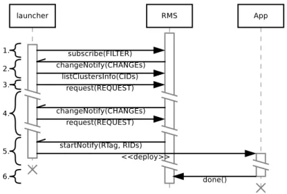
NDRMSaa consists of one or more applications, their launchers and the RMS. Since the interac-tion between the launcher and the applicainterac-tion itself is programming-model dependent and does not involve the RMS, we focus on the protocol between the launcher and the RMS (Figure 1). Let us first define some abstract data types:
• FILTER is a JSDL-like filter to select candidate clusters. It specifies the minimum number of hosts, per-host RAM, total RAM, scratch space etc.
Figure 1: Relationships between application launchers and RMS.
Figure 2: Example of interactions between the RMS, an application and its launcher. • CINFO (cluster info) is a structure containing information regarding a cluster, for example
the number of hosts, the number of CPUs per host, number of cores per CPU, size of RAM, size of scratch space, access to secondary storage facilities etc.
• ICINFO (inter-cluster info) stores information about the interconnection of one or more clusters, for example network topology, bandwidth and latency. This information can either be manually entered by the administrator or could be computed by a Network Weather Service [18]. In very complex networks Vivaldi coordinates [19] can be provided. • COP (Cluster Occupation Profile) represents the occupation of a cluster as a function of
absolute time.
• REQUEST describes a resource request, i.e. which resources the application wants and for how long. For example, a REQUEST might specify the number of hosts on each cluster and a wall-time.
• RID (resource ID) uniquely identifies a resource, e.g. a hostname.
• RTag (request tag) is an opaque type, allowing the RMS to inform the application which resource request has been granted.
• CHANGE represents a change event for a cluster. It is composed of the tuple { CID, type, COP }, where type specifies whether cluster information, inter-cluster information and/or the occupation profile has changed. In the first two cases, the application shall pull the information it requires using the interface provided by the RMS. In the latter case, the new COP is contained in the message.
In addition, plurals are used to denote “set of” (e.g. CIDs means “set of CID”).
A typical communication example of how a single application (through its launcher) interacts with the RMS is displayed in Figure 2: 1) The launcher subscribes to the resources it is
interested in. Depending on the input of the application, the launcher might use the filter to eliminate unfit resources like hosts with too little memory or unsupported architectures. 2) The RMS registers the application in its database and sends a changeNotify message with the relevant clusters and their COPs. Since the launcher has no previous knowledge about the clusters, it has to pull the CINFOs by calling listClustersInfo. 3) Using this information, the launcher computes a resource request and sends it to the RMS. 4) Until these resources become available and the application can start, the RMS keeps the application informed by sending changeNotify messages every time information regarding the resources or the occupation of resources change. The launcher recomputes the request of the application, if necessary. 5) When the requested resources become available, the RMS sends a startNotify message, containing the RIDs that the application may use. 6) Finally, when the application has finished, it informs the RMS that the resources are freed by sending a done message.
For multiple applications, each launcher creates a separate communication session with the RMS. No communication occurs between the launchers. It is the task of the RMS to compute for each of them a view, so that the goals of the system are met.
4.3 Discussion
This section has presented NDRMSaa, an abstract architecture for delegating scheduling to applications. Regarding the targeted features in Subsection 3, flexibility has been obtained by allowing resource selection to be done by the application. The RMS still keeps control of the resources, as it grants access to resources and decides what view to present to each application. The abstract architecture does not guarantee that the other criteria are satisfied. In order to insure that the system is scalable and fair, a more concrete design has to be devised.
5 Blueprint
This section presents NDRMSbp a blueprint for the NDRMSaa abstract architecture. First, more concrete data types are described. Second, the support for three types of application is studied, which are later used for the evaluation. Third, the core of the RMS is detailed, and particularly its scheduling algorithm. Four, how the targeted criteria are satisfied is discussed. 5.1 Data Types
This subsection gives more precise definitions for the abstract data types introduced in Subsec-tion 4.2.
Resources are allocated at the host granularity, so that applications do not share network and memory bandwidth, and are better isolated. This simplifies resource management, by allowing resource occupation to be represented as the number of busy hosts on each cluster. A COP is stored as a sequence of steps, each step storing a duration and a number of hosts. To avoid problems related to delays in distributed systems, a COP uses absolute time coordinated, e.g. expressed as a Unix time-stamp.
With this simplification, hosts inside a cluster are equivalent. Therefore, REQUEST shall contain the number of requested hosts on each cluster. The RMS is responsible for choosing the host IDs, which are sent to the application as RIDs in the startNotify message.
The exact information which has to be provided in CINFO and ICINFO is outside the scope of this paper. However various sources of inspiration could be used, such as GLUE [20], Grid’5000 API [21] or Adage [22]. This paper assumes that they contain enough information so that an application can select resources appropriately.
(a) (b) (c) (d) (e)
Figure 3: Scheduling example for a single-cluster moldable application. 5.2 Application-side Scheduling
Let us study some examples of how applications—rigid, simple-moldable and complex-moldable (CEM)—can use the RMS-provided information to compute a resource request which minimizes their response time. For all applications, the changeNotify handler has to read the information sent by the RMS and update the locally stored view of the resources. Then each application runs a specific algorithm to send a new request. Rigid applications are treated as a particular case of simple-moldable applications, as a result the latter are presented first.
5.2.1 Simple-moldable Applications
Let us consider a single-cluster moldable application model similar to [23], which is described by the minimum (nHmin) / maximum (nHmax) number of hosts, the proportion of the program that can be parallelized (P ∈ [0, 1]) and the single-host duration on the ith cluster (d(i)
1 ). Given
a cluster i and the number of hosts (nH), its wall-time (d(i)nH) can be computed according to
Amdahl’s law:
d(i)nH = (1− P + P /nH)· d(i)1
Let us give an example, inspired by [1], of how the launcher of such an application may use its view to compute a resource request. Assume there is a single cluster with 5 hosts with the COP presented in Figure 3(a) and a simple-moldable application with P = 1, nHmin = 1,
nHmax =∞ and d(1)1 = 5. For each cluster in the view, the launcher shall iterate through the list
of steps (which start at 0, 1 and 2). For the first step at 0, there are 4 free hosts; however, these 4 hosts will not be available during the whole length of the computed wall-time (Figure 3(b)). For the same step at 0, the launcher will retry, with the minimum number of free hosts it has previously found (1 host) and obtains an end-time of 5 (Figure 3(c)). For the step at 1, it has 1 free host and obtains an end-time of 6. For the step at 2, there are 5 free hosts and the end-time is 3, which is the best that can be obtained: the launcher chooses to request 5 hosts.
The detailed pseudo-code of this algorithm is presented in Appendix A.2.
5.2.2 Rigid Applications
Let us consider a single-cluster rigid application, which is characterized by a fixed number of hosts nHr and a wall-time d(i)r for each cluster i it can run on. Scheduling such an application is
done using the same simple-moldable application launcher, using parameter P = 1, d(i)1 = d(i)r ·nH
and nHmin= nHmax = nHr.
5.2.3 Complex-moldable Applications
Let us consider a multi-cluster iterative application like the CEM application presented in [4], which has its own, specialized resource selection algorithm. Scheduling this type of application
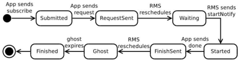
Figure 4: Application states inside the RMS in NDRMSbp.
can be done similarly to the moldable application, except that the COPs of all the clusters have to be simultaneously considered. The pseudo-code is given in Appendix A.3.
5.3 RMS-side Scheduling
This section describes the blueprint of the RMS. First, the behavior of the RMS during its interaction with an application is described. Some of the steps trigger the scheduling algorithm, which is presented next.
Fairness is maintained by delaying the deallocation of resources, so that applications with lengthy resource selection algorithms have a chance (if necessary) to send a new request. Appli-cation launchers need to know about these resources which are artificially kept busy, otherwise they might take suboptimal decisions. Maintaining a consistent view for application launchers is achieved using “ghosts” which are described below.
5.3.1 Interaction
During the interaction with the application launchers (Figure 2), the RMS has to accomplish two tasks: update the view of each application and schedule them based on their current resource requests.
Figure 4 presents the state diagram of an application inside the RMS. An application is considered to enter in the system when it calls subscribe for the first time, its initial state being Submitted. The RMS then sends it the current resource occupation (we shall call this the last view), which associates to each CID a COP with the number of hosts that are occupied as a function of time. The last view is either empty or has been previously computed.
Once the application sent its first request, it is transitioned to the RequestSent state, where it awaits scheduling. The RMS runs its scheduling algorithm and computes the estimated start time of the application. The scheduling algorithm also updates the views of all applications and marks for each application the set of “dirty clusters”, i.e. the set of clusters whose COPs have changed. After this step, the application is transitioned to the Waiting state.
If, after running the scheduling algorithm, the estimated start time of the application is the current time, this means that enough resources are available. The application is transitioned to the Started state and a startNotify message is sent to it. The message contains the set of allocated hosts, which is generated by arbitrarily choosing hosts from the list of each cluster’s free hosts.
When the application finishes, as a result of a done message, it is first transitioned to the Ghost state, where it still uses up resources. We chose this solution to improve fairness (Sec-tion 3). Without this state, the scheduling algorithm would immediately start the next applica-tion that requested the newly freed resources, without allowing any higher-priority applicaapplica-tion to adapt and possibly request the resources which are about to be freed.
The ghost is kept in the system for a fair-start amount of time. After the ghost has ex-pired, the application is transitioned to the Finished state, where all its associated resources are deallocated and returned to the list of each cluster’s free hosts.
1. Check whether there are applications which sent done and mark them as ghosts. 2. Check whether there are ghosts which have expired and mark them as finished. 3. Generate the initial last view by adding the Started applications and Ghosts to it.
4. For all RequestSent and Waiting applications, taken in the order of their submission time: (a) Set the application’s view to the last view;
(b) Compute the application’s estimated start time, i.e. the first hole in the last view, where its request would fit for the specified wall-time;
(c) Add its request to the last view; (d) Mark the application as Waiting.
5. Send changeNotify messages to applications whose view has changed because of the previous steps.
Figure 5: Scheduling algorithm of the RMS in NDRMSbp.
5.3.2 Scheduling
The scheduling algorithm of the RMS (Figure 5) is run every time a request message is received or when a ghost expires. However, to coalesce multiple such events and reduce overhead, a re-scheduling timer has to expire before the next re-re-scheduling.
The scheduling algorithm is inspired by the one used in OAR, which is first-come-first-serve (FCFS) with repeated back-filling [24]. Note that this is different from the algorithm commonly known as Conservative Back-Filling (CBF) as it does not guarantee start times. The algorithm was specifically chosen for two reasons. First, events always propagate from high-priority applications to low-priority ones (priority being given based on the time the first resource request was sent). Therefore the system eventually converges. This has the potential to reduce message exchanges between the RMS and applications, which is good for scalability. Second, this paper does not insist on scheduling issues, but on a better collaboration between the RMS and applications. Therefore, it makes sense to “imitate” an existing RMS as a basis for the evaluation. Other scheduling algorithms could be implemented (e.g. [16]), provided they enable the system to converge.
5.4 Discussion
Section 4 showed that the architecture itself guarantees flexibility and authoritativeness. Let us discuss the other two criteria: scalability and fairness.
By construction, NDRMSbp guarantees that the system converges. While this is a de-sired property, it does not guarantee that the system scales. The communications might be prohibitive, or the cost of the schedules that have to be computed might be too expensive. NDRMSbp has two parameters which could reduce the load of the system: the re-scheduling timer and the number of applications considered during scheduling.
Increasing the re-scheduling timer lowers the reactivity of the system. However it also lowers the number of times the scheduling algorithm is invoked. Since the views of the applications are changed only after re-scheduling, communication is also decreased. Limiting the number of applications considered during scheduling also limits the system load as it reduces the number of applications the RMS negotiates with (e.g. it takes only the first 200 applications in the queue). However, this would worsen resource utilization as fewer applications can back-fill the resources. The next section evaluates the scalability of NDRMSbp from both computation and communication point-of-view to see if these parameters need to be tuned.
Regarding fairness, the “ghost” mechanism ensures that in a loaded system, applications have some time to adapt and to request the resources which are about to be freed. However, in
Figure 6: Metrics measured in the experiments.
a lightly loaded system there are no ghosts and unfairness might appear. For example, let an application A arrive at t = 0 and B arrive at t = 1. If A requires 2 s to compute a request and B can instantly send a request, B could be started on the resources that A would have requested, thus penalizing A for having a lengthy resource selection. This limitation of NDRMSbp and the small unfairness it introduces is deliberately tolerated, as the alternative—blocking all resources of the platform, even for a short time—seems worse. Note that, the “ghost” mechanism only blocks resources which are used by an application, which is a smaller subset of all the resources. For example, the ghost of a single-cluster application blocks only a single cluster which is only a fraction of a dozen clusters. Fairness is controlled using the fair-start delay parameter. The higher the value, the more time applications have to adapt (and thus fairness is increased). However resources are wasted as the size of the “ghosts” in the system increases. The trade-off between fairness and resource efficiency is also studied in the next section.
6 Evaluation
This section evaluates NDRMSbp using a Python home-made simulator called NDRMSsim. It first focuses on scalability and then on fairness.
6.1 Scalability
Let us first introduce some metrics and highlight their importance for scalability. Next, these metrics are measured for two sets of experiments: one which compares NDRMSbp to an OAR-like RMS using applications with simple resource selection, and one which studies NDRMSbp when complex applications are included.
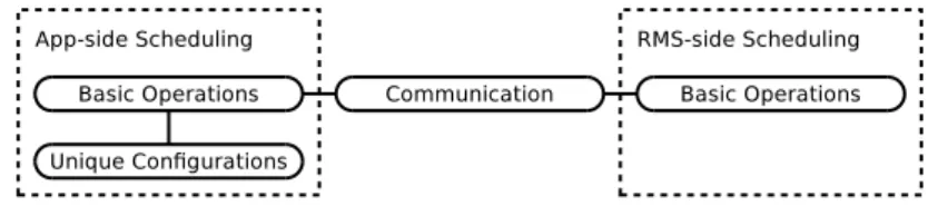
Metrics Figure 6 shows the main metrics that are measured and their relationship to the
actors of the mentioned systems. Basic operations is a measure of the complexity of the involved scheduling algorithms; it is defined as the number of COP steps that have been iterated. The more basic operations, the higher the underlying processor usage will be. Since a real implementation might choose to run the launchers and the RMS on different processors, the application-side, RMS-side and sum of the two are shown. Reducing the number of RMS-side operations seems more important as the RMS is a bottleneck.
Since it is difficult to tie the number of basic operations to the CPU usage of a real-life implementation, the simulation time1is given. This metric indicates how much CPU time it takes
to schedule a workload, assuming the whole system runs on a single core. Since the simulator is written in Python, this metric should only be taken as a hint, as a real implementation should be a lot faster.
Unique configurations represents how many configurations the applications had to compute, assuming that a caching mechanism avoids duplicate configurations. This metric is important for applications with lengthy resource selection algorithms.
Both OAR and NDRMSbp require the launchers and the RMS to communicate. If the launchers reside on different machines than the RMS, a large amount of communication might
turn the front-end’s network into a bottleneck. This is less of a concern if the RMS and the launchers run on the same machine, as they could use shared memory for efficient communica-tion. To measure bytes, messages are encoded similarly to CORBA’s CDR [25], using long for wall-times and host-counts, and byte for CIDs. Detail can be found in Appendix B.1.
All the above metrics are computed as total over an experiment, instead of averaging over time, as we feel that it makes the results more meaningful and less dependent on the chosen workload. Indeed, multiplying the execution/wall-times of the applications of a workload by a large number (e.g. 100) would not change the totals, but the averages would be significantly reduced.
Experiments The first set of experiments focuses on how NDRMSbp scales with the
com-plexity of the resources. Rigid and simple-moldable applications are selected, which can be scheduled both by exhaustively enumerating their moldable configurations (having a limited number of configurations) and by delegating scheduling to them. Both an OAR-like RMS and NDRMSbp are used to obtain equivalent schedules. Hence, by comparing these two systems, the overhead that scheduling delegation adds can be characterized.
The second set of experiments studies how NDRMSbp scales with the number of complex applications, by introducing complex-moldable (CEM) applications in the workload. The com-parison with OAR is dropped as the required number of configurations for these applications becomes too large.
In both sets of experiments, the fair-start timer of NDRMSbp is set to 5 seconds. Its influence is studied later. The re-scheduling timer has been set to 1 second, as this is a good starting value for a very reactive RMS.
6.1.1 Comparison between OAR and NDRMSbp
NDRMSbp is compared to an OAR-like RMS, since, to our knowledge, it is the only RMS with support for moldable applications, which can also be used in a multi-cluster environment2. We implemented an OAR simulator (OARsim), in which the applications submit all their configura-tions and the RMS greedily choses the configuration which leads to the earliest completion-time, similarly to OAR’s core scheduling algorithm.
Resource Model Resources are made of nC clusters, each having 128 hosts. The ith cluster
(i∈ [2, nC]) is considered 1 + 0.1· (i − 1) times faster than cluster 1.
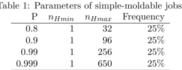
Application Model To generate a workload, we used the first 200 jobs of the LLNL-Atlas-2006-1.1-cln
trace from the parallel workload archive [26]. We took the number of processors and the execution-time of these jobs and generated rigid jobs with probability 1 − pmo. The other pmo are considered simple-moldable with the parameters shown in Table 1. The single-host
execution-time of a simple-moldable application on the first cluster is computed according to Amdahl’s law: d(1)1 = d/(1− P + P /nH), where d, nH are the values of the run-time and
processor-count found in the traces.
In NDRMSaa, the launcher is aimed to choose a (more-or-less precise) wall-time. Therefore, we chose not to use the wall-times provided with the original traces, as they are mostly set to the system’s default wall-time. For all the above applications, the wall-time is equal to the execution-time multiplied by a uniform random number in [1.1, 2].3 The job arrival rate is of 1
application per second, as we want to test the system when the load is high. 2http://oar.imag.fr/users/user_documentation.html
3Experiments have been done using the default wall-times. While NDRMSsim performed a little worse, the results remain within the same order of magnitude.
Table 1: Parameters of simple-moldable jobs. P nHmin nHmax Frequency
0.8 1 32 25%
0.9 1 96 25%
0.99 1 256 25%
0.999 1 650 25%
Analysis for a Single Cluster We first analyze the single-cluster case (nC = 1) where the
number of simple-moldable jobs varies according to the pmo parameter.
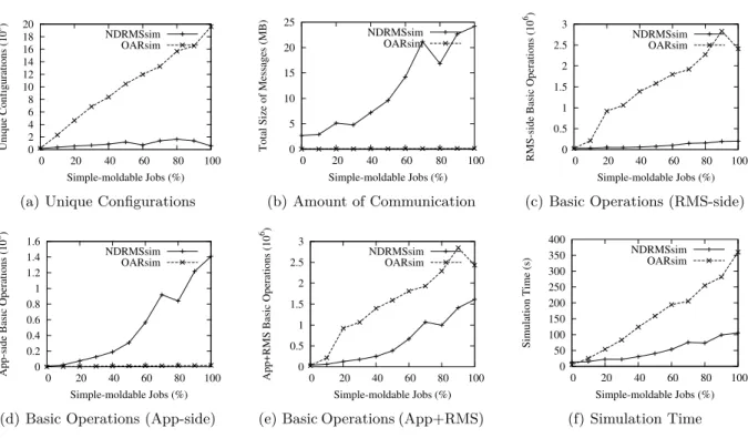
Figure 7(a) shows that NDRMSbp reduces the number of unique configurations the appli-cations have to compute. The more simple-moldable appliappli-cations are in the system, the higher the benefit is. This happens because launchers only need to compute configurations which are encountered during scheduling and do not have to exhaustively enumerate them. While it is not very important for the Amdahl law based moldable application of the experiments, since computing one Amdahl formula is not costly, it becomes more important for applications which employ complex algorithms to compute their configurations, such as the CEM application.
If the launchers and the RMS are run on the same machine, NDRMSbp is able to reduce the total number of basic operations (Figure 7(e)), thus potentially reducing the CPU usage. We observe this metric is strongly correlated to the simulation time (Figure 7(f)) in which NDRMSbp also outperforms the OAR-like RMS. NDRMSbp required up to 100 s to schedule 200 applications (less than 1 s per application), which suggests an efficient behavior.
Figure 7(c) and 7(d) show that in comparison to OAR, NDRMSbp makes fewer operations on the RMS’s side, but more operations on the applications’ side, as a result of delegating scheduling decisions to the applications. If the launchers are run on a separate machine than the RMS, NDRMSbp reduces the congestion on the front-end, while the communication is more demanding than in the case of OAR (Figure 7(b)). In the worst case, a total of 25 MB of data have to be exchanged by NDRMSbp to fulfill its task (an average of 125 KB per application). While it is more that one would usually expect, it is our opinion that with today’s networks this is hardly an issue.
When there are only rigid applications in the system, all metrics (except the number of App-side basic operations and communication) are similar for the two systems. It stems from the fact that, on one cluster, rigid applications have only one single configuration, thus they do not adapt.
To sum up, results show that NDRMSbp is at least as good as an existing system to support both legacy applications and somewhat more complex applications, on homogeneous resources. Delegating application scheduling turns out not to degrade system performance.
Analysis for Multiple Clusters Let us now focus on how OAR and NDRMSbp behave
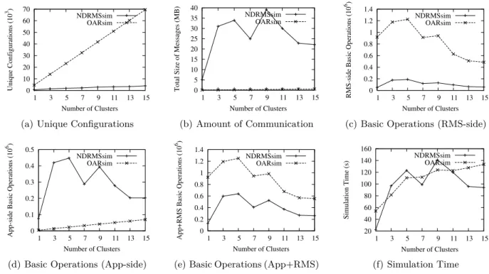
when the complexity of the resources (i.e. the number of clusters) increases. The case pmo= 20, which is representative for the data we gathered, is analyzed.
For both rigid and simple-moldable applications, the number of unique configurations they have to submit to OAR is linear in the number of clusters (Figure 8(a)). NDRMSbp scales better and the number of unique configurations increases linearly with a smaller slope.
For the number of basic operations (Figure 8(c), 8(d), 8(e)) and communication (Figure 8(b)), the same observations apply as in the single-cluster case. As the number of clusters increases, NDRMSbp scales better than an OAR-like RMS, thus potentially reducing the front-end’s CPU usage, especially when the launchers are run on separate hosts. In that case, NDRMSbp would have to exchange up to 40 MB of data (an average of 200 KB per application), which, as we previously concluded, should not be a concern for today’s systems.
0 2 4 6 8 10 12 14 16 18 20 0 20 40 60 80 100 Unique Configurations (10 3) Simple-moldable Jobs (%) NDRMSsim OARsim
(a) Unique Configurations
0 5 10 15 20 25 0 20 40 60 80 100
Total Size of Messages (MB)
Simple-moldable Jobs (%) NDRMSsim OARsim (b) Amount of Communication 0 0.5 1 1.5 2 2.5 3 0 20 40 60 80 100
RMS-side Basic Operations (10
6)
Simple-moldable Jobs (%) NDRMSsim
OARsim
(c) Basic Operations (RMS-side)
0 0.2 0.4 0.6 0.8 1 1.2 1.4 1.6 0 20 40 60 80 100
App-side Basic Operations (10
6)
Simple-moldable Jobs (%) NDRMSsim
OARsim
(d) Basic Operations (App-side)
0 0.5 1 1.5 2 2.5 3 0 20 40 60 80 100
App+RMS Basic Operations (10
6)
Simple-moldable Jobs (%) NDRMSsim
OARsim
(e) Basic Operations (App+RMS)
0 50 100 150 200 250 300 350 400 0 20 40 60 80 100 Simulation Time (s) Simple-moldable Jobs (%) NDRMSsim OARsim (f) Simulation Time Figure 7: Simulation results for a single cluster.
The number of basic operations and the communication increase up to a certain point, but seems to remain constant after that, as we are in the case of weak scalability and the number of applications is constant.
Regarding simulation time (Figure 8(f)), for NDRMSbp it is still well correlated to the total number of basic operations. However, in OAR’s case we observe a much weaker correlation. The two systems end up having similar simulation times, which suggests that they would equally load the CPU of the front-end, if the launchers ran on the same machine. 150 s were required to schedule 200 applications (less than 1 s per application) which, as we previously stated, is an acceptable value.
To conclude, NDRMSbp also scales well with the complexity of the resources and is a good choice to schedule simpler application on them.
6.1.2 Delegating Scheduling of Complex Applications
The second set of experiments studies whether NDRMSbp scales with the number of complex applications in the system. The comparison with an OAR-like RMS is completely dropped, as the number of possible configurations for a multi-cluster application is 129nC (one can choose
between 0 to 128 hosts independently on each cluster), which even for a few clusters is imprac-tical.
Application Model We started from the application model used in the previous set of
ex-periments. We fixed pmo = 20, since we have already studied the influence of this parameter.
Let W 0 be this workload.
Two workloads (W 1 and W 2) are derived from W 0: in W 1, a CEM application is inserted at position nCEM for testing how NDRMSbp behaves in a somewhat realistic workload: 79.6%
rigid, 19.9% simple-moldable, 0.5% (1 out of 201) complex-moldable applications. In W 2, some applications are replaced (with a certain probability) by CEM applications, to observe how NDRMSbp scales with the number of complex applications.
0 10 20 30 40 50 60 70 1 3 5 7 9 11 13 15 Unique Configurations (10 3) Number of Clusters NDRMSsim OARsim
(a) Unique Configurations
0 5 10 15 20 25 30 35 40 1 3 5 7 9 11 13 15
Total Size of Messages (MB)
Number of Clusters NDRMSsim OARsim (b) Amount of Communication 0 0.2 0.4 0.6 0.8 1 1.2 1.4 1 3 5 7 9 11 13 15
RMS-side Basic Operations (10
6)
Number of Clusters NDRMSsim
OARsim
(c) Basic Operations (RMS-side)
0 0.1 0.2 0.3 0.4 0.5 1 3 5 7 9 11 13 15
App-side Basic Operations (10
6)
Number of Clusters NDRMSsim
OARsim
(d) Basic Operations (App-side)
0 0.2 0.4 0.6 0.8 1 1.2 1.4 1 3 5 7 9 11 13 15
App+RMS Basic Operations (10
6)
Number of Clusters NDRMSsim
OARsim
(e) Basic Operations (App+RMS)
20 40 60 80 100 120 140 160 1 3 5 7 9 11 13 15 Simulation Time (s) Number of Clusters NDRMSsim OARsim (f) Simulation Time Figure 8: Simulation results for multiple clusters with pmo = 20.
Resource Model In addition to the resource model used for our previous set of experiments, a model for the network that interconnects the clusters is also needed. We chose to group every two clusters in a “city” and every two “cities” in a “country”. The latency between two clusters is 5 ms if they are in the same city, 10 ms if they are in the same country, and 50 ms otherwise. While running CEM applications on Grid’5000, the latency was the main factor limiting scalability [4]. Thus, we assume all clusters have infinite bandwidth, to reduce simulation time.
Analysis For W 1, we ran experiments for nCEM = 1, . . . , 200. Since the results of these
experiments are similar, this paper only analyzes those for nCEM = 40. For W 2, we ran simulations for pCEM = 0.1, 0.2, . . . , 1. Similarly, only significant experiments are reported, i.e
for pCEM ∈ {0.2, 0.5, 0.8, 1}.
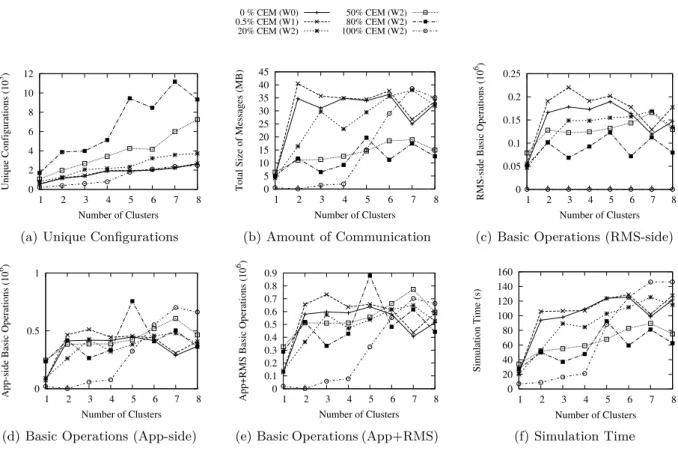
The most important observation is that the total number of unique configurations scales well, both with the number of complex applications and the complexity of the resources (Figure 9(a)). Computing a CEM configuration can take up to 200 ms. To run a single CEM application on an OAR-like system, one would need to enumerated 129nC unique configurations. Even for
three clusters, this value would be equal to 2, 146, 689, which is a lot greater than 12, 000, the maximum number of unique configurations obtained with NDRMSbp for nC = 8.
The total number of unique configurations, computed by all applications, is increasing until there are 80% of CEM applications in the system. After 80%, the number of unique configura-tions decreases and reaches a relatively low level when 100% of the applicaconfigura-tions are CEM. This is due to the fact that the CEM launchers try to request as many hosts from a cluster as pos-sible. So when the number of rigid and simple-moldable applications is decreasing, scheduling CEM applications is reduced to selecting entire clusters for them, which reduces the number of configurations which have to be calculated. Note that this behavior is very specific to this workload and other applications (for example those that do not select whole clusters) might not make the system exhibit this behavior.
The number of RMS-side, application-side and total basic operations (Figures 9(c), 9(d) and 9(e)) slightly increase when a complex application is introduced in the system (W 1 vs. W 0).
0 % CEM (W0) 0.5% CEM (W1) 20% CEM (W2) 50% CEM (W2) 80% CEM (W2) 100% CEM (W2) 0 2 4 6 8 10 12 1 2 3 4 5 6 7 8 Unique Configurations (10 3) Number of Clusters
(a) Unique Configurations
0 5 10 15 20 25 30 35 40 45 1 2 3 4 5 6 7 8
Total Size of Messages (MB)
Number of Clusters (b) Amount of Communication 0 0.05 0.1 0.15 0.2 0.25 1 2 3 4 5 6 7 8
RMS-side Basic Operations (10
6)
Number of Clusters
(c) Basic Operations (RMS-side)
0 0.5 1
1 2 3 4 5 6 7 8
App-side Basic Operations (10
6)
Number of Clusters
(d) Basic Operations (App-side)
0 0.1 0.2 0.3 0.4 0.5 0.6 0.7 0.8 0.9 1 2 3 4 5 6 7 8
App+RMS Basic Operations (10
6)
Number of Clusters
(e) Basic Operations (App+RMS)
0 20 40 60 80 100 120 140 160 1 2 3 4 5 6 7 8 Simulation Time (s) Number of Clusters (f) Simulation Time Figure 9: Simulation results for NDRMSbp including complex-moldable applications. However when adding more such complex applications, these metrics tend to decrease due to the previously described workload characteristic.
The simulation time (Figure 9(f)) suggests that even if all launchers run on the front-end, the system should be able to deal with the load even as resources are increasingly complex. At most 150 s were required to schedule the 200/201 applications, which is quite small, considering that the CEM resource selection algorithm is included.
Assuming launchers are run on separate hosts, the RMS does not need to execute more basic operations as the complexity of the workload increases (Figure 9(c)). This means that applica-tions with complex resource requirements can be supported with a simple RMS-side scheduling algorithm. In such a configuration there is a significant amount of data being transfered between the RMS and the applications (Figure 9(b)). At most 45 MB had to be transfered (about 230 KB per application), which should be an acceptable value for today’s networks. This value is small compared to the amount of data required to exhaustively enumerate all configurations. On 8 clusters, a multi-cluster application would require 613, 490 TB according to our encoding.
This experiment has shown that NDRMSbp has reached its goal of scheduling complex-moldable applications on complex resources in a scalable manner.
6.2 Fairness
This subsection studies the importance of the fair-start delay parameter, which should be set by system administrators. It first discusses how a minimum value should be chosen, to maintain the fairness properties of NDRMSbp, then the associated resource waste is analyzed.
6.2.1 Maintaining Fairness
For this experiment, the resource model from Section 6.1.2 is kept the same (with nC
0 0.2 0.4 0.6 0.8 1 1.2 1.4 5 10 15 20 25 30 End Delay (10 3 s) Adaptation Delay (s) CEM End Delaying (Average)
0 20 40 60 80 100 120 140 160 180 5 10 15 20 25 30 End Delay (10 3 s) Adaptation Delay (s) CEM End Delaying (Maximum)
Figure 10: Unfairness caused by insufficient fair-start delay.
0 0.5 1 1.5 2 2.5 3 3.5 5 10 15 20 25 30
Resource Waste (s * host * 10
6) Fair-Start Delay (s) 0% CEM 20% CEM 50% CEM 80% CEM 100% CEM
Figure 11: Resource waste for nC = 4.
following differences: the rigid and simple-moldable jobs were generated from 200 randomly-chosen, consecutive applications in the original workload traces and a complex-moldable CEM application is inserted into the workload at a uniform randomly chosen position between 1 and 200.
To simulate an application with a lengthy resource selection algorithm, an adaptation de-lay was added to the CEM application launcher, which means that, after having received a changeNotify message, it delays sending its new resource request with that amount of time.
Figure 10 shows both the average and the maximum of the end delay, i.e. the number of seconds the CEM application finished later compared to a zero adaptation delay. We observe that having a fair-start delay smaller that the adaptation delay seriously worsens the CEM application’s scheduling performance, both on average and in extreme cases. This happens because other applications, with zero adaptation delay, occupied the resources that the CEM application could have taken advantage of (had it adapted faster), thus increasing its finish time. In order to maintain fairness, the administrator of the system should choose the fair-start delay so that all applications have time to adapt or at least communicate that parameter to users so that they use adequate scheduling algorithms.
6.2.2 Resource Waste
Let us study how many resources are wasted as a function of the fair-start delay and the number of multi-cluster (CEM) applications. The metric to be studied is the resource waste, defined as the total number of second-hosts occupied by “ghosts”. We chose this metric as an absolute value (and not a percentage of the applications’ execution time), so that the conclusions be less workload dependent.
The chosen resource and the application model are the same as in Section 6.1.2, more exactly W 2 (for pCEM ∈ {0, 0.2, 0.5, 0.8, 1}) is used. nC = 4 is taken as other values of nC give fairly
similar results.
Figure 11 shows that, as expected, the resource waste increases linearly with the fair-start delay. The higher the number of multi-cluster applications, the bigger the resource waste. The number of applications being kept constant, the more clusters (and implicitly hosts) the application launchers request, the more resources each ghost will occupy.
In the worst case (fair-start delay of 30 s, 100% of CEM applications), the execution of 200 applications wasted 3 million second-host, each of the 512 hosts being idle for about 1.5 h. Depending on the average execution time of the applications, this value might be acceptable or not. For example, the trace we have taken for the evaluation, has an average job runtime of 1.5 h. Thus, 0.5% of the resources would be wasted, for a fair-start delay of 30 s, which is quite small. In contrast, if the average job runtime is 5 min, 10% of the resources would be wasted.
6.3 Discussion
This section evaluated the NDRMSbp blueprint through simulations. The results showed that the system scales well if up to 200 applications are being scheduled, without the need of increasing the re-scheduling timer. In a real-life system, the maximum number of scheduled applications should either be an administrative parameter, or the system should dynamically choose a value for it.
An administrator has to reach a compromise between resource waste and fairness. Ideally, the fair-start delay should be set to a high enough value so that all complex applications have time to adapt.
7 Validation
This section presents NDRMSi a proof-of-concept implementation of NDRMSbp. It first presents NDRMSi and how it differs from NDRMSsim, then it presents some metrics mea-sured with it to validate the simulations.
7.1 Description
NDRMSi has been developed by branching of from NDRMSsim. Besides changing the sim-ulated sleep functions with real system calls, the three following changes have been made: i) RMS-Application communication has been ported to omniORBpy4 a popular CORBA imple-mentation. The IDL has been written straight-forward from the blueprint. ii) Since omniORBpy may run servants in separate threads, the state variables have been protected by a lock. iii) Handling of protocol violations have been added. If the launcher of an application is unrespon-sive or the application exceeds its wall-time, it is killed by being transitioned to the FinishSent state. Unresponsive launchers are detected using CORBA exceptions.
The applications are only sleeping, no deployment nor real execution takes place on the allocated resources.
7.2 Comparison between NDRMSsim and NDRMSi We ran NDRMSi with a workload similar to W 25 (p
CEM = 0, 0.2, 0.5, 0.8, 1) and the resource
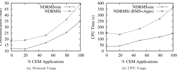
model of Section 6.1.2 (for nC = 8) has been selected. We measured the CPU-time consumed by the RMS and the sum of sent and received TCP payload to/from the RMS. The RMS was run on the first processor, while all the launchers were run on the second processor of a system with two single-core AMD Opteron™ 250 processors, running at 2.4 GHz.
Figure 12(a) compares the network traffic generated by NDRMSi with the simulation results. Values obtained in practice are up to 50% higher than those obtained in theory. This is caused mainly because of CORBA’s IIOP overhead, but also because we neglected some messages in the simulations. However, the generated traffic is of the same order of magnitude, therefore we argue that the scalability from the network perspective is validated, even if the RMS and the launchers run on separate hosts.
Figure 12(b) compares the simulation time with the CPU-time consumed by the whole system (RMS and launchers). Practical values are up to 3.3 times higher than simulations. However this is to be expected. Every time communication occurs, data needs to be converted from Python’s representation to CORBA’s and back. Also, the measured CPU-time includes starting up the launchers which, due to the need of loading the Python executable and compiling the
4Python frontend of OmniORB:http://omniorb.sourceforge.net/.
5To reduce the time of the experiments, we skipped over the trace-file jobs whose area (size× run-time) was larger than 7200 processor× seconds. The total number of jobs was kept at 200.
10 15 20 25 30 35 40 45 50 0 20 40 60 80 100 Communication (MB) % CEM Applications NDRMSsim NDRMSi
(a) Network Usage
0 50 100 150 200 250 300 350 400 0 20 40 60 80 100 CPU Time (s) % CEM Applications NDRMSsim NDRMSi (RMS+Apps) (b) CPU Usage Figure 12: Comparison between NDRMSsim and NDRMSi.
byte-code, is quite high. Nevertheless, the burden on the CPU is quite low, which proves that NDRMSi scales well.
8 Conclusion
This paper addressed the issue of scheduling complex applications on complex resources (i.e. grids), by completely delegating resource selection to the applications. Results show that the approach is feasible and a prototype implementation serves as a proof-of-concept.
The proposed architecture assumes that the RMS is centralised, as the central point of this paper is to studying the high-level requirements of non-describable applications. Future work should focus on splitting this RMS into a local RMS and a global RMS, as is commonly found in today’s computing grids.
We proposed allocating computing resources at host granularity. In future, we would like to study the implications of allocating resources at CPU core granularity.
[15] and [16] propose limiting the number of available resources an application should choose from. This approach could be implemented in NDRMSi’s RMS-side scheduling algorithm, how-ever the consequences should be studied.
9 Acknowledgement
This work has been supported by the ANR COOP project: http://coop.gforge.inria.fr/. Experiments presented in this paper were carried out using the Grid’5000 experimental testbed, being developed under the INRIA ALADDIN development action with support from CNRS, RE-NATER and several Universities as well as other funding bodies (see https://www.grid5000. fr).
References
[1] J. Hungershofer, “On the combined scheduling of malleable and rigid jobs,” in SBAC-PAD ’04: Proceedings of the 16th Symposium on Computer Architecture and High Performance Computing. Washington, DC, USA: IEEE Computer Society, 2004, pp. 206–213.
[2] G. Staples, “TORQUE resource manager,” in SC ’06: Proceedings of the 2006 ACM/IEEE conference on Supercomputing. New York, NY, USA: ACM, 2006, p. 8.
[3] K. Keahey, M. Tsugawa, A. Matsunaga, and J. Fortes, “Sky Computing,” IEEE Internet Computing, vol. 13, no. 5, pp. 43–51, 2009.
[4] E. Caron, C. Klein, and C. Pérez, “Efficient grid resource selection for a CEM application,” in RenPar’19. 19ème Rencontres Francophones du Parallélisme, Toulouse, France, Sep. 2009.
[5] G. Alliance, “Resource specification language.” [Online]. Available: http://www.globus. org/toolkit/docs/4.0/execution/wsgram/schemas/gram_job_description.html
[6] Global Grid Forum, “Job Submission Description Language (JSDL) Specification.” [Online]. Available: http://www.gridforum.org/documents/GFD.56.pdf
[7] N. Capit, G. Da Costa, Y. Georgiou, G. Huard, C. Martin, G. Mouni´e, P. Neyron, and O. Richard, “A batch scheduler with high level components,” CoRR, vol. abs/cs/0506006, 2005.
[8] E. Elmroth and J. Tordsson, “A grid resource broker supporting advance reservations and benchmark-based resource selection,” in PARA, 2004, pp. 1061–1070.
[9] A. Sulistio, W. Schiffmann, and R. Buyya, “Advanced reservation-based scheduling of task graphs on clusters,” in Proc. of the 13th Intl. Conference on High Performance Computing (HiPC), 2006.
[10] H. Mohamed and D. Epema, “Experiences with the KOALA co-allocating scheduler in mul-ticlusters,” in IEEE International Symposium on Cluster Computing and the Grid (CC-Grid2005), vol. 2. IEEE Computer Society Press, May 2005, pp. 784–791.
[11] W. Smith, I. Foster, and V. Taylor, “Scheduling with advanced reservations,” in In Pro-ceedings of IPDPS’00, 2000, pp. 127–132.
[12] H. Casanova, “Benefits and drawbacks of redundant batch requests,” Journal of Grid Com-puting, vol. 5, no. 2, pp. 235–250, 2007.
[13] G. Graciani Diaz, A. Tsaregorodtsev, and A. Casajus Ramo, “Pilot Framework and the DIRAC WMS,” in CHEP 09, Prague Tch`eque, R´epublique, May 2009.
[14] F. Berman, R. Wolski, H. Casanova, W. Cirne, H. Dail, M. Faerman, S. Figueira, J. Hayes, G. Obertelli, J. Schopf, G. Shao, S. Smallen, N. Spring, and A. Su, “Adaptive computing on the grid using AppLeS,” 2003.
[15] S. Srinivasan, V. Subramani, R. Kettimuthu, P. Holenarsipur, and P. Sadayappan, “Effec-tive selection of partition sizes for moldable scheduling of parallel jobs,” in High Performance Computing — HiPC 2002, ser. Lecture Notes in Computer Science, S. Sahni, V. Prasanna, and U. Shukla, Eds. Springer Berlin / Heidelberg, 2002, vol. 2552, pp. 174–183.
[16] S. Srinivasan, S. Krishnamoorthy, and P. Sadayappan, “A robust scheduling strategy for moldable scheduling of parallel jobs,” IEEE Intl. Conference on Cluster Computing, p. 92, 2003.
[17] P. Bar, C. Coti, D. Groen, T. Herault, V. Kravtsov, A. Schuster, and M. Swain, “Running parallel applications with topology-aware grid middleware,” Intl. Conference on e-Science and Grid Computing, pp. 292–299, 2009.
[18] R. Wolski, N. T. Spring, and J. Hayes, “The network weather service: A distributed re-source performance forecasting service for metacomputing,” Journal of Future Generation Computing Systems, vol. 15, pp. 757–768, 1999.
[19] R. Cox, F. Dabek, F. Kaashoek, J. Li, and R. Morris, “Practical, distributed network coordinates,” SIGCOMM Comput. Commun. Rev., vol. 34, no. 1, pp. 113–118, 2004. [20] G. G. Forum, “GLUE specification v. 2.0,” Mar. 2009. [Online]. Available: http:
//www.ogf.org/documents/GFD.147.pdf
[21] “Grid’5000 API.” [Online]. Available: http://www.grid5000.fr/mediawiki/index.php/API [22] S. Lacour, C. P´erez, and T. Priol, “A network topology description model for grid
appli-cation deployment,” in Proc. of the 5th IEEE/ACM Intl. Workshop on Grid Computing (GRID 2004), R. Buyya, Ed., Pittsburgh, PA, USA, Nov. 2004, pp. 61–68.
[23] Y. Caniou, G. Charrier, and F. Desprez, “Evaluation of Reallocation Heuristics for Mold-able Tasks in Computational Dedicated and non Dedicated Grids,” Institut National de Recherche en Informatique et en Automatique (INRIA), Tech. Rep. RR-7365, Aug. 2010. [24] A. W. Mu’alem and D. G. Feitelson, “Utilization, Predictability, Workloads, and User
Runtime Estimates in Scheduling the IBM SP2 with Backfilling,” IEEE Transactions on Parallel and Distributed Systems, vol. 12, no. 6, pp. 529–543, 2001.
[25] O. M. Group, Common Object Request Broker Architecture (CORBA / IIOP), Version 3.1, Jan. 2008. [Online]. Available: http://www.omg.org/spec/CORBA/3.1/
[26] “The parallel workloads archive.” [Online]. Available: http://www.cs.huji.ac.il/labs/ parallel/workload
A Application-side Scheduling
A.1 Operations with COPsLet a cluster occupation profile (COP) be a sequence of steps, each step being characterized by a duration and a number of nodes. Formally, cop = {(d1, n1), (d2, n2), . . . , (dN, nN)}, where N is
the number of steps, di is the duration and ni is number of nodes of step i. For manipulating COPs, we use the following helper functions:
• cop(t) returns the number of nodes at time coordinate t,
i.e. cop(t) = n1 for t∈ [0, d1[, cop(t) = n2 for t∈ [d1, d1+ d2[, etc.
• max(cop, t0, t1) returns the maximum number of nodes between t0 and t1
i.e. max(cop, t0, t1) = maxt∈[t0,t1[cop(t), and 0 if t0= t1.
• loc(cop, t0, t1) returns the end time coordinate of the last step containing the maximum,
restricted to [t0, t1] i.e. loc(cop, t0, t1) = t⇒
max(cop, t0, t) = max(cop, t0, t1) > max(cop, t, t1).
• cop1+ cop2 is the sum of the two COPs, i.e. ∀t, (cop1+ cop2)(t) = cop1(t) + cop2(t).
• chps(cop) returns the set of time coordinates between steps (change-points) i.e. chps(cop) = (d0, d0+ d1, d0+ d1+ d2, . . .).
A.2 Scheduling a Moldable Application
The pseudo-code for computing the resource request of a moldable application is presented in Algorithm 1:
1. The change-points of all COPs are iterated in increasing order (line 4);
2. For each change-point cluster pair, check if the minimum number of required hosts are free and compute the wall-time according to Amdahl’s law (line 9).
3. Next, use the getMaxNodes() method to check whether enough host are available during the computed wall-time (lines 10–11).
(a) If enough hosts are available, update the best found end time, wall-time, cluster ID and number of hosts (lines 14–18).
(b) If not, the number of hosts is updated (line 12) and a new wall-time is computed, until either a fitting request has been found, or less than nHmin hosts are available.
input : n(cid) : number of hosts on cluster cid
cop(cid) : occupation of cluster cid
d(cid)0 : single-host wall-time on cluster cid
output: cidbest, nbest, dbest : resource request which should be sent to the RMS, i.e.
cluster, number of hosts and wall-time that minimises completion-time
begin
1
tbestCompletionT ime=∞;
2
chpCl← list of (change-point, cid) tuples (in increasing change-points order);
3
for ts, cid∈ chpCl do
4
if tbestCompletionT ime< ts then
5
break;
6
nH ← n(cid)− cop(cid)(ts);
7
/* Until we find a nH that fits at this change-point */ while nH ≥ nHmin do 8 d← (1 − P + P /nH)· d (i) 0 ; 9
n0H ← n(cid)− max(cop(cid), t
s, ts+ d); 10 if n0H < nH then 11 nH ← n0H; 12 else 13
/* Update best request */
if ts+ d < tbestCompletionT ime then
14
tbestCompletionT ime← ts+ d;
15
cidbest← cid;
16 nHbest← nH; 17 dbest← d; 18 break; 19
return cidbest, nbest, dbest
20
end
21
A.3 Scheduling a CEM Application
The pseudo-code for scheduling the CEM application in [4] is presented in Algorithm 2. We assume we have a resource selection function f0, which gets as input acid representing the number
of available hosts on cluster cid and outputs a list of selected hosts scid (representing the desired
number of hosts on each cluster — possibly zero) and a wall-time d.
The algorithms is similar to the one that schedules moldable applications, but differs in the fact that it tracks the number of hosts on multiple clusters at the same time. The acid,∀cid
sequence keeps for each cid the number of available hosts, which is then used when calling f0. The algorithm works as follows:
1. acid is initialized with the number of available hosts at moment when the algorithm is
started (line 4);
2. The change-points of all COPs are iterated in increasing order (line 6);
3. For each change-point cluster pair, update a (line 10) and call f0(line 12), to get a wall-time d and the set of selected resources s;
4. Next, use the getMaxNodes() method to check whether enough host are available during the computed wall-time (lines 13–18); this check is done for all the clusters selected by f0; (a) If enough hosts are available, update the best found end time and request (lines 19–
24);
(b) If not, the number of hosts is updated (line 17) and a new wall-time is computed, until either a fitting request has been found, or no resources are available (line 14); 5. The algorithm stops when a change-point is after the best found completion time (line 9).
input : n(cid) : number of hosts on cluster cid
cop(cid) : occupation of cluster cid f0 : resource selection function
output: nbest={ncid0, ncid1, . . .}, dbest : resource request which should be sent to the RMS, i.e. number of hosts on each cluster and wall-time that minimises completion-time
begin
1
now→ time at which the algorithm is started;
2
/* Initialize number of available hosts for each cluster */
for cid∈ CIDs do
3
acid ← n(cid)− cop(cid)(now);
4
tbestCompletionT ime=∞;
5
chpCl← list of (change-point, cid) tuples (in increasing change-points order);
6
for ts, cid∈ chpCl do
7
if tbestCompletionT ime< ts then
8
break;
9
/* Update number of available hosts for this cluster */ acid ← n(cid)− cop(cid)(ts);
10
/* Until we have hosts */
while∃i, ai ≥ 0 do
11
s, d← f0(a) ;
12
/* Check whether the selected resources fit for the desired
duration */
f its← T rue ;
13
for∀cid, scid > 0 do
14
n0H ← n(cid)− max(cop(cid), ts, ts+ d);
15 if n0H < nH then 16 acid ← n0H; 17 f its← F alse; 18 if fits then 19
/* Update best request */
if ts+ d < tbestCompletionT ime then
20 tbestCompletionT ime← ts+ d; 21 rbest← cid; 22 dbest← d; 23 break; 24
return rbest, dbest
25
end
26