A Study of the Process-Spatial Link in Ice Pressure-Area Relationships

Publisher’s version / Version de l'éditeur:

PERD/CHC Report 7-108, 2004-03-20

READ THESE TERMS AND CONDITIONS CAREFULLY BEFORE USING THIS WEBSITE.

https://nrc-publications.canada.ca/eng/copyright

Vous avez des questions? Nous pouvons vous aider. Pour communiquer directement avec un auteur, consultez la Questions? Contact the NRC Publications Archive team at

PublicationsArchive-ArchivesPublications@nrc-cnrc.gc.ca. If you wish to email the authors directly, please see the first page of the publication for their contact information.

Archives des publications du CNRC

For the publisher’s version, please access the DOI link below./ Pour consulter la version de l’éditeur, utilisez le lien DOI ci-dessous.

https://doi.org/10.4224/12340936

Access and use of this website and the material on it are subject to the Terms and Conditions set forth at

A Study of the Process-Spatial Link in Ice Pressure-Area Relationships

Daley, C.

https://publications-cnrc.canada.ca/fra/droits

L’accès à ce site Web et l’utilisation de son contenu sont assujettis aux conditions présentées dans le site LISEZ CES CONDITIONS ATTENTIVEMENT AVANT D’UTILISER CE SITE WEB.

NRC Publications Record / Notice d'Archives des publications de CNRC:

https://nrc-publications.canada.ca/eng/view/object/?id=fc4bc9fe-2e07-4b1d-bbd9-792b5edda929 https://publications-cnrc.canada.ca/fra/voir/objet/?id=fc4bc9fe-2e07-4b1d-bbd9-792b5edda929

Prepared for

National Research Council of Canada By

Claude Daley

Faculty of Engineering and Applied Science Memorial University of Newfoundland

March 20, 2004 St. John's, NF, A1B 3X5 Canada

A

A

S

S

t

t

u

u

d

d

y

y

o

o

f

f

t

t

h

h

e

e

P

P

r

r

o

o

c

c

e

e

s

s

s

s

-

-

S

S

p

p

a

a

t

t

i

i

a

a

l

l

L

L

i

i

n

n

k

k

i

i

n

n

I

I

c

c

e

e

P

P

r

r

e

e

s

s

s

s

u

u

r

r

e

e

-

-

A

A

r

r

e

e

a

a

R

R

e

e

l

l

a

a

t

t

i

i

o

o

n

n

s

s

h

h

i

i

p

p

s

s

TABLE OF CONTENTS

Symbols

Acknowledgement

1 Introduction...1

2 Description of Ice Contact ...3

2.1 General ...3

2.2 Spatial Pressure Distribution...4

2.3 Process Pressure Distribution...6

2.4 Link Between Process and Spatial Distributions...7

3 Polar Sea Data ...8

3.1 Description of the Pressure Measurement System ...8

3.2 Polar Sea Data Reduction...10

3.3 Polar Sea Data Analysis ...11

3.3.1 Data From the 1982 Trials ...13

3.3.2 Data From the 1983 Trials ...16

3.3.3 Summary of ’82 Plots ...19

3.3.4 Summary of ’82 And ’83. ...20

3.4 Discussion of Polar Sea Data. ...21

4 Numerical Contact Model ...24

4.1 Model Development ...24 4.2 Simulation Results ...25 4.3 Discussion...27 5 Conclusions...28 6 Recommendations ...28 7 References ...29 Annex A - Polar Sea 1982 Event Summary.

Annex B - Polar Sea 1983 Event Summary.

Annex C - Example of Polar Sea Event Data Files.

Annex D - Example of Polar Sea Spatial & Process Pressure-Area Event Files.

Symbols

A

_Area

_m

A

total contact area

m

C

_Ice

_pressure

_constant

_MPa

_at

_1m

e

_{Area exponent in the pressure}

_-

P

_{Ice Pressure}

_MPa

P

average ice pressure in the contact area MPa

F

Force

MN

Table of Figures

Figure 1. Sketch of ice contact with a structure...3

Figure 2 Sketch of ice pressure and the meaning of a specific pressure-area plot...4

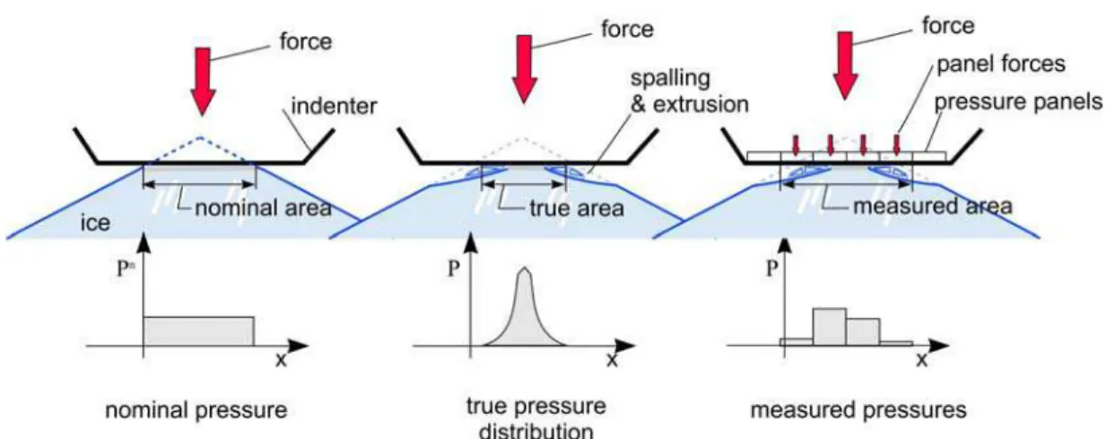
Figure 3. Types areas and pressures related to pressure-area data...5

Figure 4. Sketch of measured ice pressure data and spatial pressure-area plots. ...5

Figure 5. Sketch of measured ice pressure data and process pressure-area plots. ...6

Figure 6. Combined spatial and process pressure-area data. ...7

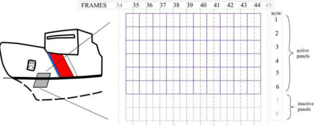
Figure 7. Ice load panel as installed in the Polar Sea...8

Figure 8. Ice load panel layout on the Polar Sea...9

Figure 9. Illustrative example of the spatial pressure-area calculation with Polar Sea data. ...11

Figure 10. Example of analysis plots on one event from the Polar Sea trials (the data in this plot is artificial)...12

Figure 11. Re-analyzed data from event #135, from 1982. This was the highest force event in the ’82 trials. ...13

Figure 12. Re-analyzed data from event #114, from 1982. This was the 2nd highest force event in the ’82 trials. ...14

Figure 13. Re-analyzed data from event #137, from 1982. This was the 3rd highest force event in the ’82 trials. ...15

Figure 14. Re-analyzed data from event #410, from 1983. This was the highest force event in the ’83 trials. ...16

Figure 15. Re-analyzed data from event #366, from 1983. This was the 2nd highest force event in the ’83 trials. ...17

Figure 16. Re-analyzed data from event #215, from 1983. This was the 4th highest force event in the ’83 trials. ...18

Figure 17. Compilation of pressure trend plots for 1982 Polar Sea data. ...19

Figure 18. Compilation of pressure trend plots for 1983 Polar Sea data. ...19

Figure 19 Comparison of pressure trend plots for 1982 and 1983 Polar Sea data. ...20

Figure 20. Assemblage of measured pressure area data. ...21

Figure 21. Assemblage of Pressure-area data with example spatial and process pressure-area curves from the 1982 Polar Sea trials. ...22

Figure 22. Influence of the e and C terms in the process pressure-area relationship. ...23

Figure 23. Contact Failure Process Model [19]. The contact process is modeled by a discrete sequence of through-body cracks. ...24

Figure 24. Contact/Extrusion model from [2]...25

Acknowledgement

The work was made possible with the support of funding from PERD (Panel on Energy Research

and Development). The author wishes to thank Dr. Garry Timco of the NRC/CHC (Canadian

Hydraulics Centre) for his support and patience.

1 Introduction

Ice is the dominant feature in artic waters for most or all of the year. In sub-artic regions, ice can

be present in many forms for part of the year. The eastern coastal waters in Canada are prone to

extensive ice coverage. Ice will often be the dominant load when considering the design of ships

and offshore structures for many regions, including in the Gulf of St. Lawrence, Newfoundland

waters and along the Labrador coast. Many see ice as the dominant design challenge, and in

other cases, the primary impediment preventing the economic development of resources.

Consequently, improving our understanding of ice loads is a topic of large practical significance.

Ice loads on structures occur over a specific, often quite small area. The area of contact is, more

or less, the area of overlap of the ice edge and the structure. The earliest measurements and

models were primarily concerned with the total ice contact force. Early ice load models [6] did

include terms to show that the average ice pressure varied, but there was no representation of

pressure variation within the contact. As an approximation, the pressure within the contact was

assumed uniform.

The interest in ice loads grew significantly in the 1970s and 80s, as offshore oil and gas

developments expanded. From about 1980 onwards, there have been many field trials and

measurements in which ice loads have been measured [8,9,10,11,12,13,14,15]. These include ice

loads on ships and offshore structures. Many of these experiments and trials were able to

measure the distribution of pressure within the contact area. This lead to the realization that ice

pressure is far from uniform. To a degree far greater than with wind and current loads, ice

pressure measurements depended on the size of the sensor, especially for quite small sensors. To

describe this effect, the pressure data was often plotted with area as the independent variable.

Investigators began to see area as one of the dominant, if not the dominant, determinant of ice

pressure. Parameters such as ice strength, thickness, and velocity, tended not to vary much in any

data set and thus had less influence on pressure. On the other hand, pressures on small sensors

(for example a few square centimeters) were observed to be orders of magnitude higher than

pressures measured on large sensors (square meters). As more data became available, the

pressure-area plot became the most common way to present ice pressure data [16].

Today, pressure-area (p/a) models are commonly used to determine both local and global ice

loads on ships and structures.

There are two distinct types of pressure-area models [4,18]. The ‘process’ p/a

distribution describes how the average pressure relates to the total contact area, and is used to

calculate the collision force. The ‘spatial’ p/a model is a description of how local peak pressures

relate to area for areas within the total contact. The ‘spatial’ model is used to determine design

loads on local structure, such as plating and framing.

This report examines the link between the two pressure-area models. Evidence from both field

measurements (e.g. Polar Sea [1]) and numerical models (e.g. NEB/PERD report [2]) appears to

relationship is unclear. It is not certain that the average pressure declines as the total area

increases, as is often assumed. This has a very significant impact on the calculated maximum

loads. Coupled with the link to local (spatial) pressures, there is a question about the proper level

of design pressures in situations involving large forces.

To clarify this last point, let us consider design of an offshore structure for iceberg impact. All

available p/a panel data has been gathered in cases where the total force is less than about 20MN,

with almost all data for cases below about 5MN. While there is some pressure data for very large

forces, such data only gives the overall average pressure, not the pressure distribution, and comes

from cases of very large aspect ratio. Such data is of little value when studying the general nature

of ice loads. In the case of iceberg impact, calculated forces can easily be in the range of 50 MN

and up to several hundred MN. Such predicted loads and pressures cannot be empirically

validated directly. The values are an extrapolation of the data, and rely on the relationships

inherent in the pressure-area models. If the average pressure rises with area, calculated pressures

become significantly larger than for constant or declining pressures. Further, if local pressures

are strongly correlated with total force, the local pressures in a large iceberg collision may be

higher, even significantly higher, than any measured to date. The two effects combine to create

an important question.

Thus, there are significant practical implications to a linkage between the two p/a curves. This

report will examine the pressure-area data from the Polar Sea to study this linkage. As well, a

numerical model of contact will be examined from this perspective to see if it can shed light on

this issue.

2 Description of Ice Contact

2.1 General

Figure 1 shows an idealized sketch of the contact between a large ice feature and a structure. All

items except the flexural crack will be present in every ice contact, though to varying extents.

The ice exerts pressure on the structure both directly and through a layer of extruding crushed

ice. The highest pressure will occur in the direct solid contact. The ice in the solid contact region

may be damaged by internal cracks and material damage, but is quite confined and capable of

sustaining very high pressures. Towards the edge, the structure is only in contact with crushed

and extruded rubble and will exert quite low pressures. The pressures may well vary over many

orders of magnitude within the contact region. Outside the contact, the pressures are effectively

zero. The sketch may describe an event that is only centimeters across, or it may be meters

across. This report examines the ice pressures that occur in situations such as this.

2.2 Spatial Pressure Distribution

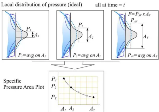
The spatial pressure distribution describes the variation of pressure in an ice contact at one

instant in time. Figure 2 illustrates the idea. The pressure varies within the contact, forming one

or more peaks. The highest pressure occurs on a small area at the peak. The average pressure

within larger areas will necessarily be smaller than the peak pressure. Average pressures over

progressively larger areas (each containing all the smaller area and more) well decline.

Consequently, spatial pressure-area plots will always show an inverse relationship between

pressure and area. Typically, such relationships take the form:

P=C

A

(1)

where C is a positive value, representing the average pressure at one unit of area, and e is in

the range 0..1. C is typically in the range of 0.5 to 5 MPa and e is typically be in the range of –

0.25 to –0.7 . The values vary from dataset to dataset.

Figure 2 Sketch of ice pressure and the meaning of a specific pressure-area plot.

There are several ways to define both pressure and area, and then the meaning can be affected by

the measurement procedure. We are rarely able to measure with both fine spatial resolution and

large areal coverage. As a result, the data tends to be coarse and may obscure the real trends.

Figure 3 illustrates three variations of the meaning of the word pressure, and associated area. On

the left, we define ‘nominal pressure’. If we have independently measured the total force, and we

have observed the overlap area (nominal area) of the ice and structure, we can divide one by the

other and find the nominal pressure. This is a useful value, but gives no information on the local

surface with high spatial resolution. This type of data is practically non-existent. The right hand

sketch shows the situation that we normally face. The pressure has been measured on a rather

coarse array, and may be subject to noise and other forms of error. Consequently, the coarseness

of the array and the data collection/reduction algorithms can influence the estimates of the local

pressures. There are always some pressure and areal resolution limits to deal with. These points

should be kept in mind when thinking about ice load data. Figure 4 shows the spatial

pressure-area plat that would be derived from measured values.

2.3 Process

Pressure

Distribution

At any point in time, there is a total area, and an average pressure. The product of these two

values is the force. Figure 5 illustrates the process pressure-area plot, as would be derived from

measured data using an array of pressure sensors.

Referring again to Figure 3 it is obvious that the measured average pressure and the measured

total area is similar to the nominal pressure. In cases where there is no independent measure of

both total force and nominal area, the values as would be estimated in Figure 5 are the only way

to determine the nominal values. This is an important point. Nominal pressure area values are

required for those cases in which the design load is estimated from an impact analysis. This is the

case for iceberg-structure collision and many ship-ice collision loads. No field data has both

complete coverage with pressure panels, and independent measurement of force and nominal

contact. Such a data set would allow force to be determined by two independent measurements.

All the extensive data from ships only contain pressure panel measurements. Consequently, we

are left with the measured process pressure-area values as often the only estimate of the nominal

pressure-area relationship. It is hoped that future ice load data collection programs will be able to

gather both types of data.

Figure 5 illustrates another point about the process pressure-area relationship. Unlike the spatial

pressure-area relationship, there is no a-priori reason for the pressure to fall with increasing area.

Factors such as increasing confinement could well lead to increasing average pressures as the

interaction proceeds. Most authors have suggested declining trends [16], yet others have

suggested rising trends [7, 13].

2.4 Link between Process and Spatial Distributions

The spatial and process pressure area plots are derived from the same data. The process values

are just the average pressures over all the measured sensors (the non-zero pressures). Figure 6

shows both types of data on the same plot. This again illustrates how the spatial pressure area

curve can be falling, even as the process curve is rising. Note that the connection between the

two types also suggests that higher local pressures will tend to occur with greater total areas and

total contact forces.

3 Polar Sea Data

3.1 Description of the pressure measurement system

Figure 7 shows a sketch of the instrumented portion of the bow of the Polar Sea [8]. An array of

strain gauges was placed on 10 structural frames in the bow of the ship. The location was chosen

to give the highest chance of large collisions. Each of ten frames was instrumented with 8 strain

rosettes. The primary measurement was compressive strain normal to the shell. The gauges were

placed in such a way give continuous coverage within the panel, and yet be is insensitive as

possible to pressures outside the local region. Cross-over effects were removed by the use of a

matrix of influence factors derived by finite element analysis. The measurement system was

validated by means of a physical calibration.

Figure 7. Ice load panel as installed in the Polar Sea.

The actual panel layout is shown in Figure 8. Each sub-panel was 0.152 m

, and the total panel

covered 9.1 m

. The strain gauges were sampled 32 times per second. Each event began when a

threshold level of ice pressure was read. Once triggered, the event was sampled for the same

amount of time. The event lasted from one second before the trigger to approx. 4 seconds after

the trigger.

1

Figure 8. Ice load panel layout on the Polar Sea

Annex A and B show a partial summary of the events. The largest panel pressures and forces are

listed for the 1982 and 1983 trials in Multi-year ice. Annex C shows an example of the pressure

data in a single event file. The full records are available in electronic form.

3.2 Polar Sea Data Reduction

The Polar Sea data, after conversion, is a set of panel pressures. In its original form [21], these

are in units of p.s.i., stored as an integer. Each time step contains 60 values, referring to the six

rows on each of ten frames. There are either 158 or 200 time steps per event, and there are

thousands of events.

The data was analyzed initially in a number of ways. The force on the panel was found by

summing the sub-panel forces (product of pressure and area). Thus a force time history of the

collision could be plotted. Peak force and peak pressures were tabulated for each event. Similar

values were found for each row and frame (to be used to assess loads on transverse and

longitudinal frames). For each of the events, a spatial pressure-area plot was calculated for two

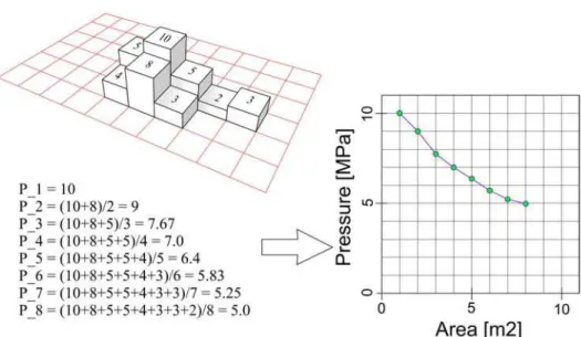
cases; the time of peak force, and the time of peak pressure. Figure 9 shows how the spatial

pressure-area plots are calculated.

For the present project the data from the Beaufort Sea trials of 1982 and the Chukchi Sea trials of

1983 were re-analyzed. These trials contain mainly collisions with large multi-year ice floes. For

a large selection of events the pressure records were re-analyzed to give a spatial pressure-area

data for every time step. The highest force events were included. With the spatial pressure-area

data at every time step, it was then possible to extract the process pressure-area data, which

required the total area and average pressures. The process pressure-area data were divided into

two parts. The first part was during rising force, which is presumably while ice penetration

occurs. The second part was while the force declined, when presumably the penetration was over

and rebound and slide-off occurred. To use the data as a basis for extrapolation to larger

collisions, it is reasonable to separate these two types of data. This data is only plotted for that

part of the event when the main activity (the main impact) occurred. This further helps to clarify

the processes that occur during collision from the general ‘noise’ that occurs before and after.

Figure 9. Illustrative example of the spatial pressure-area calculation with Polar Sea data.

3.3 Polar Sea Data Analysis

The Polar Sea data has been re-analyzed to extract both spatial and process pressure-area curves.

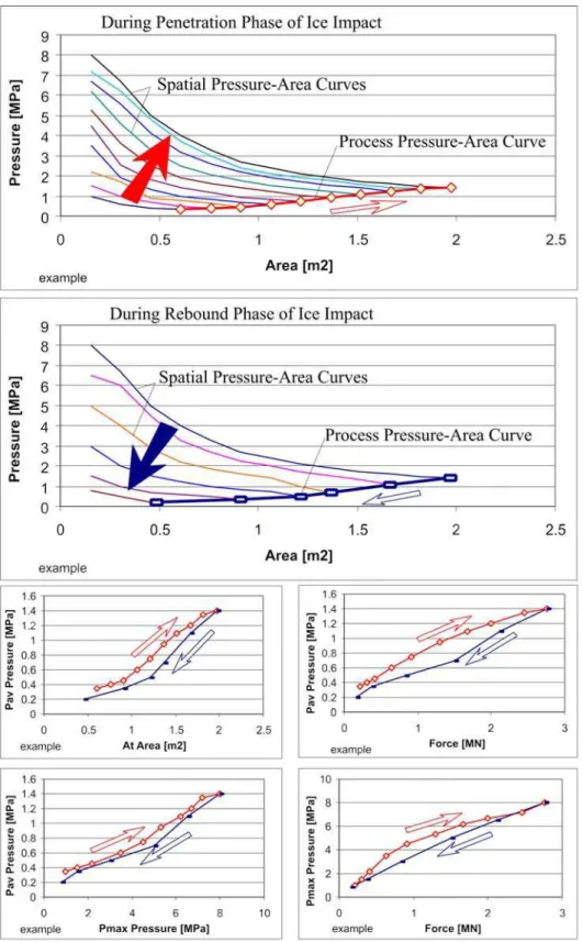
Figure 10 illustrates the types of analysis plots for an example data set (which is similar to an

actual data set, but with less noise). The top plot is a set of spatial pressure-area curves during ice

penetration phase of the impact, along with the process pressure area curve for that event. As can

be seen, the peak pressures (closest to the pressure axis) rise as the whole curve rises, and as the

total area rises. The process pressure-area curve is found by joining the ends of the spatial p-a

curves. The process p-a curve rises in both pressure and area. The total force at each step from

the product of the values of the process curve (pressure x area). The second plot illustrates the

case during the declining part of the impact. The declining plots will not be included for the

actual data, as they serve little purpose here. The four smaller plots below show the various

relationships between average pressure, total area, total force and peak pressure. In the example

all four of these quantities rise together. The plots show both the rising and falling values.

In Figure 11, 12 and 13 re-analyzed data is shown from the three largest events from the 1982

Beaufort Sea trials. All show trends that are similar to the idealized example, with all values

rising together.

Figure 10. Example of analysis plots on one event from the Polar Sea trials (the data in this

plot is artificial).

3.3.1 Data from the 1982 Trials

Figure 11. Re-analyzed data from event #135, from 1982. This was the highest force event

in the ’82 trials.

Figure 12. Re-analyzed data from event #114, from 1982. This was the 2

highest force

event in the ’82 trials.

Figure 13. Re-analyzed data from event #137, from 1982. This was the 3

highest force

event in the ’82 trials.

3.3.2 Data from the 1983 Trials

Figure 14. Re-analyzed data from event #410, from 1983. This was the highest force event

in the ’83 trials.

Figure 16. Re-analyzed data from event #215, from 1983. This was the 4

highest force

event in the ’83 trials.

3.3.3 Summary of ’82 Plots

The plots in Figure 17 show the relationships among average pressure, total area, force and peak

pressure for the five largest events during the 1982 trials. All events show similar trends, the

most important being that average pressure rises as area and force increase. Similarly, the peak

pressure rises as well.

Figure 17. Compilation of pressure trend plots for 1982 Polar Sea data.

The plots in Figure 18 show the relationships among average pressure, total area, force and peak

pressure for the five largest events during the 1983 trials. As before, all events show similar

trends.

3.3.4 Summary of ’82 and ’83.

Figure 19 compares the 1982 and 1983 data sets. While following similar trends the two data sets

do not match. The 1982 data shows higher average pressure. One can only speculate as to the

cause of the difference. One obvious cause would be that the two data sets were from different

times of the year (Oct. in 1982 and April in 1983). The only odd aspect of this is that the

weather was warmer in October and so, presumably, was the ice. Could it be that warmer ice

caused higher average pressures? This idea runs counter to the usual trend with ice strength.

However, given that the colder ice may have been more brittle (and ‘dry’ as crushed ice was

extruded), it may make sense that the warmer ice produced higher average pressures. This is a

very curious result and deserves further attention.

3.4 Discussion of Polar Sea Data.

The Polar Sea data has shown some interesting and potentially important trends. When the data

from experiments is all plotted together, the plot appears to show an inverse relationship between

pressure and area. This is because the plot is primarily showing the spatial pressure area

relationship. Further, when sets of data are grouped and plotted, an inverse pressure-area

relationship is also often seen in the upper envelope of the data. Unfortunately, such a trend is

only a reflection of the limited level of force in the various data sets. Pressure and area can never

be truly independent variables, because pressure is really force per unit area. A line of constant

force will appear as an inverse relationship between pressure and area.

Most of the empirical evidence we have for pressure-area trends comes from impact tests of

quite limited force. Either the ram has limited force capacity, or the vessel has limited

energy/momentum. Consequently, any assemblage of events from a given set of similar

experiments will almost certainly be constrained by a level of force. When plotted, such data will

necessarily show an envelope with an inverse relationship between pressure and area. Such a

trend has absolutely no meaning when one is attempting to extrapolate to situations involving

larger loads. In effect, our limited experience with large forces is falsely showing us that

pressures (and forces) will stay small. Figure 20 [10] shows a plot of most available pressure

area data. The cloud to the left of the plot tends to be from the kind of low aspect ratio impacts

that are of interest here. An envelope line, often assumed to be highly conservative, is shown.

The analyses presented above have attempted to determine the true pressure-area relationships as

they occur when ice and structure are in contact. When the penetration phase of the collision is

isolated for single impacts, we see a surprising trend. The average pressure rises as the force and

contact area rise during the collision. This is to say that the process pressure-area curves rise, not

fall. This is a very significant result. Figure 21 shows how some of the process pressure area

curves from the Polar Sea compare to the general data. From this it would appear that ice

pressure in high force collisions could be well above anything observed to date.

Figure 21. Assemblage of Pressure-area data with example spatial and process

pressure-area curves from the 1982 Polar Sea trials.

By way of illustration, take the case of an ice mass of 80 kT striking a vertical wall at 2 m/s.

Assuming the edge radius of 15 m, the force is readily calculated from energy considerations [5].

The calculation requires that the process pressure-area equation is known. Figure 22 shows the

dramatic changes in estimated ice collision force that occur as e changes from –1 to 0 to +1. The

constant C has a relatively minor effect by comparison. One might imply a value +0.5 for e, from

the Polar Sea data. For the case shown below, this would result in a predicted force as almost 100

times greater that that obtained for a value of e=-0.7. Such a potential error is astounding. Of

course, such an event might well be limited by another failure mechanism. Nevertheless, this

possibility deserves further analysis.

4 Numerical Contact Model

This chapter will examine the process and spatial pressure-area curves from the perspective of a

numerical model of ice edge contact. The model is a 2D model of contact, and this is a

significant issue. The model was developed to help understand and explain certain laboratory

experiments that were essentially 2D. The model may help to explore the issues, but can not be

expected to model the general 3D impacts that occurred when the Polar Sea struck multi-year

floes.

4.1 Model

Development

The first version of the model used here was developed in [19] with only direct contact and

flaking aspects considered. That model was well able to simulate and explain many observed

phenomena in a set of lab experiments [20] involving crushing contact on large blocks of sea ice.

Figure 23 shows the model as first developed. The model was able to explain the following key

observations/phenomena in the Joensuu-Riska tests: multi-sawtooth force time-history, crushed

particle piece size distribution, pressure-area (process) time history, local (spatial) pressures,

observed direct contact geometry (line), and the variations in force records between successive

experiments (i.e. the ‘randomness’, that was not actually random). This numerical simulation

was able to explain the observed pressure-area curves without resorting to an assumption of

random strength properties.

Figure 23. Contact Failure Process Model [19]. The contact process is modeled by a

discrete sequence of through-body cracks.

A refinement of the above model was developed in [2] (see Annex E for listing), that added the

consideration of an active extrusion rubble zone above and below the central contact point. In the

refined model, the contact face is vertical, so that the ice is in the plane of the water. With that,

contact zone and provides an initial pressure to constrain the extrusion. The extrusion zones

(between the contact face and the ice) are a series of opening wedges, each with an outlet

pressure and an inlet pressure. A simple model of extrusion of a granular material has been used

to describe the pressures in the extrusion zones.

The most important result of the inclusion of the extruded material is not the loads carried

directly by the crushed ice, but rather that influence of the confining effects of the crushed ice on

the failure of the intact ice. The intact ice fails by shearing. Pressure in the extrusion zone has the

effect of compressing the shear failures, strengthening them. This results in greater force

transmitted through the direct contact, as well as force through the crushed ice.

The intent in this report is to explore the pressure-area effects with the model.

Figure 24. Contact/Extrusion model from [2]

4.2 Simulation

Results

The model was exercised for the four conditions. Table 2 shows the key results for the relatively

thin ice sheet (2m). Table 3 shows the key results for the relatively thick (20m) ice. Both shapes

were run with and without consideration of extrusion. Extrusion can be eliminated by setting the

various friction factors (ice-ice and ice-structure) to zero. The thick ice was included to examine

the case where large 45 degree flakes do no take place. As such the ice thickness does not

actually matter.

The other model parameters are as shown in Table 1. These were not chosen for their accuracy,

but only to explore the sensitivities.

Table 1. Contact model constants

Item Description

[units]

Value(s)

Pc

direct contact pressure [MPa]

20

c

ice shear strength (Coulomb model) [MPa]

0.8

φ

ice friction angle (Coulomb - solid ice)

0º or 10º

φ

solid ice - structure contact friction angle

0º or 10º

φ

granular ice - structure friction angle

0º or 6º

φ

granular ice - ice contact friction angle

0º or 10º

sl_sail

slope of the extruded material above ice

0.8

sl_keel

slope of the extruded material below ice

0.8

rho

rubble mass density [kg/m

] 560

Table 2. Contact/Extrusion model runs for 2m sheet.

Run 1 Run 2

Geometry 2m sheet with 45º edge 2m sheet with 45º edge Extrusion included in calculations ? no yes Fracture pattern Resulting Process Pressure-Area Plot

Table 3. Contact/Extrusion model runs for 20m sheet.

Run 3 Run 4

Geometry 20m sheet with 45º edge 20m sheet with 45º edge Extrusion included in calculations ? no yes Fracture pattern Resulting Process Pressure-Area Plot

4.3 Discussion

The contact model has shown some interesting results. The influence of the extrusion mechanics

is significant. It is clear that the slope of the process pressure-area curve is dependant on both

extrusion processes and ice edge shape. This, at least in a small way, helps to explain the Polar

Sea results.

Unfortunately, there are still many problems with the software that make it difficult to examine a

variety of extrusion parameters and ice edge shapes. For wide variations in edge shape from

those shown, the program does not run. The same is true for general changes in the ice

parameters. Only with further development will this model be able to handle an arbitrary 2D ice

edge. One might also expect that only with a full 3D model will the effects such as observed in

5 Conclusions

The re-analysis of past measurements has shown some surprising results.

The pressure-area relationship in ice should not be viewed as a single phenomenon. Instead it

should be separated into spatial and process pressure-area relationships. These are not equivalent

to local and global pressure-area trends, but are rather spatial and temporal trends of pressure.

The spatial p/a curve is needed for local structural design, while the process p/a curve is used to

determine impact forces. It has been indicated here that these two effects are strongly linked, but

are essentially different.

The evidence suggests that the process p/a curve follows a rising trend in certain cases. This is in

some ways opposite of the spatial p/a curve and the usual understanding of this data. This

suggests that we may be drastically underestimating ice forces in the case of large collisions, and

consequently underestimating the local maximum pressures.

We have little of no empirical evidence for the large force impacts for which some of our

offshore structures are designed. This must be of significant concern.

6 Recommendations

1. Further analysis and re-analysis should be performed on any available pressure-area data,

specifically to look for trends in the process pressure-area relationship.

2. Other ice-mechanics based models should be used or developed to help understand what

parameters influence the process pressure-area curve, and its relationship to the spatial

curve.

3. Large field programs are needed to provide at least some empirical evidence from large

force ice impacts. These should be conducted with the highest quality data collection

systems possible, to gain a better understanding of the true nature of the contact process.

A high resolution array of surface pressure sensors is needed, along with ice shape, and

relative position throughout the impact. Independent measurement of the ice load is

highly desirable.

7 References

1. Daley, C.G. , St. John, J., Siebold, F., and Bayly, I., (1984) "Analysis of Extreme Ice Loads

Measured on USCGC POLAR SEA", Transactions, SNAME, New York, November, 1984.

2. Daley, C.G., Tuhkuri, J., and Riska, K., "Discrete Chaotic Ice Failure Model Incorporating

Extrusion Effects", Report submitted to the National Energy Board by Daley R&E and the

Helsinki University of Technology, Nov., 1996.

3. CSA S471(1992), “ General Requirements, Design Criteria, the Environment and Loads –

Code for the Design, Construction, and Installation of Fixed Offshore Structures” Canadian

Standards Association, Rexdale, Ontario.

4. Frederking, R., “The Local Pressure-Area Relation in Ship Impact with Ice” - POAC '99,

Helsinki Finland, August 1999.

5. Daley, C.G., "Energy Based Ice Collision Forces" - POAC '99, Helsinki Finland, August

1999.

6. Korzhavin, K.N., "Action of Ice on Engineering Structures" Novosibirsk, Akad. Nauk.

SSSR, 202p., CRREL Draft Translation No.260, 1962.

7. Kheysin, D.Ye., Likhomanov, V.A. and Kurdyumov, V.A., "Determination of Specific

Breakup Energy and Contact Pressures Produced by the Impact of a Solid Against Ice",

Symp. on Physical Methods in Studying Snow and Ice, Leningrad, CRREL Translation

TL539, 1973

8. Daley, C.G., St. John, J.W., Brown, R., Glen, I.F., “Ice Loads and Ship Response to Ice –

Consolidation Report”, U.S., Ship Structures Committee Report SSC-340, 1990.

9. St. John, J.W., Daley, C.G., Blount, H, “Ice Loads and Ship Response to Ice”, U.S., Ship

Structures Committee Report SR-1291, 1984.

10. Daley, C.G., “MSI Ice Loads Data - Compilation of Medium Scale Ice Indentation Test

Results and Comparison to ASPPR”, Report by Daley R&E to National Research Council,

March 1994, Transport Canada Publication Number TP 12151E.

11. Frederking, R., Blanchet, D., Jordaan, I.J., Kennedy, N.K., Sinha, N.K. and Stander, E., 1990

“Field tests of ice indentation at medium scale, ice island, April 1989” Client Report for

Canadian Coast Guard and Transportation Development Centre, By Institute for Research in

12. Frederking, R., Jordaan, I.J. and McCallum, J.S., “Field Tests of Ice Indentation at Medium

Scale - Hobson’s Choice Ice Island, 1989”, IAHR Ice Symposium, Espoo, Finland, 1990.

13. Ghoneim, G.A.M., Johansson, B.M., Smyth, M.W., Grinstead, J., “Global Ship Ice Impact

Forces Determined from Full-Scale and Analytical Modelling of the Icebreakers Canmar

Kigoriak and Robert Lemeur”, Transactions of the SNAME Annual Meeting

14. Muhonen, A., “Medium Scale Indentation Tests - PVDF pressure measurements, ice face

measurements and Interpretation of crushing video”, Client Report by Helsinki University of

Technology, Ship Laboratory, Feb.20, 1991.

15. Sandwell., “Reduction and Analysis of 1990 and 1989 Hobson’s Choice Ice Indentation

Tests Data” Final Report, Project 112588 by Sandwell Inc., Calgary, Alberta, to Conoco Inc.

Exxon Prod. Res. Co., Mobil R and D Corp. and National Research Council of Canada,

August 1992.

16. Sanderson T.J.O. 1988. Ice Mechanics - Risks to Offshore Structures. Graham and Trotman,

London, 253 pp.

17. API RP 2N (1995) “Recommended Practice for Planning, Designing and Construction of

Fixed Offshore Structures and Pipelines for Arctic Conditions” 2

Edition, American

Petroleum Institute, Dallas Texas.

18. Frederking, R. 1998. The pressure area relation in the definition of ice forces, 8th Int.

Offshore and Polar Engineering Conference, May 24-29, 1998, Montreal, Vol. II, pp.

431-437.

19. Daley, C. 1991, “Ice Edge Contact - A Brittle Failure Process Model”, Acta Polytechnica

Scandinavica, Mechanical Engineering Series No. 100, Helsinki 1991, published by the

Finnish Academy of Technology.

20. Joensuu, A., Riska, K., 1988., "Jään ja Rakenteen Välinen Kosketus"(Contact Between Ice

and Structure) Helsinki University of Technology, Laboratory of Naval Architecture and

Marine Engineering, Report M-88, Otaniemi, 1988. (in Finnish)

21. Data CD – “Polar Sea Impact Data”, produced by STC- Science and Technology

Corporation, and BMT Fleet technology.

Annex A – Polar Sea 1982 Event Summary

The table below is an extract from the summary report of the 1882 Beaufort Sea trials. Listed

below are the peak values of force and panel pressure for the largest events ranked by force. (see

accompanying CD data disk for the full summary)

Maximum

Single Time of Peak Pressure Total Event Sub-panel Peak Location Panel Number Date Time Pressure Pressure Frame Row Force

(psi) (LT) 135 10/14/1982 11:37:39 1617 33 42 5 495 114 10/12/1982 17:07:44 1053 34 39 7 489 137 10/14/1982 11:48:28 1156 37 35 5 434 91 10/10/1982 16:38:15 1464 34 44 7 433 81 10/7/1982 23:30:29 1499 32 44 5 413 122 10/13/1982 19:17:49 597 35 43 7 388 84 10/10/1982 15:44:41 980 40 43 5 384 116 10/12/1982 18:58:17 1015 33 36 3 357 37 10/2/1982 20:43:21 656 36 35 5 319 131 10/14/1982 8:31:00 638 89 36 6 317 103 10/8/1982 9:54:07 877 33 36 3 306 73 10/8/1982 7:43:40 763 33 43 5 290 61 10/3/1982 20:47:00 551 43 38 4 287 139 10/14/1982 12:46:54 782 38 37 5 286 7 10/1/1982 12:21:26 1453 22 37 3 275 78 10/7/1982 19:42:23 794 33 43 4 270 89 10/10/1982 16:36:14 1010 34 42 5 254 110 10/12/1982 16:24:33 889 63 38 7 252 83 10/10/1982 15:23:02 901 37 35 8 251 72 10/8/1982 7:31:42 817 37 42 7 247 63 10/3/1982 20:48:16 702 42 42 5 235 20 10/1/1982 21:23:29 392 83 41 3 234 10 10/1/1982 12:23:07 663 137 36 3 232 127 10/13/1982 20:14:41 1115 35 44 3 232 97 10/10/1982 18:20:07 1093 35 38 4 226 9 10/1/1982 12:22:39 472 33 41 4 225 130 10/14/1982 8:17:38 481 32 37 8 217 32 10/2/1982 20:10:03 1013 44 42 8 214 133 10/14/1982 11:30:12 1206 33 36 8 214 80 10/7/1982 23:02:29 808 65 37 8 211 120 10/12/1982 20:05:43 584 33 41 5 211 100 10/10/1982 18:43:51 569 35 44 8 210 115 10/12/1982 17:16:31 573 40 40 7 207 158 10/7/1982 18:26:30 923 33 42 3 204 35 10/2/1982 20:30:09 439 40 35 4 203 126 10/13/1982 20:10:27 642 34 42 7 203 166 10/11/1982 0:19:37 544 47 42 7 203 152 10/7/1982 17:59:31 920 146 37 7 199 6 10/1/1982 12:20:58 951 196 39 3 195 99 10/10/1982 18:41:16 1109 32 37 4 193

Annex B – Polar Sea 1983 Event Summary

The table below is an extract from the summary report of the 1983 Chukchi Sea trials. Listed

below are the peak values of force and panel pressure for the largest events ranked by force. (see

accompanying CD data disk for the full summary)

Event Ship Maximum Time Step Frame Row

Number Date Time Speed Single of Peak Number Number Total (kt) Sub-panel Pressure of Max of Max Panel

Pressure Pressure Pressure Force (psi) Time of Time of (LT)

Peak Pres Peak Pres

410 4/24/1983 16:11:59 7.79675 1141 56 42 8 491 366 4/20/1983 13:06:18 3.19728 1319 113 44 8 443 283 4/12/1983 18:14:26 7.00652 576 139 38 5 435 215 4/11/1983 8:55:30 5.57339 1011 132 39 8 393 70 4/3/1983 2:56:29 0 264 33 37 7 387 86 4/3/1983 3:07:55 0 303 33 40 5 383 276 4/12/1983 17:47:51 6.45813 680 35 43 4 377 72 4/3/1983 2:59:31 0 280 33 36 7 374 74 4/3/1983 3:00:02 0 312 35 39 8 371 85 4/3/1983 3:06:15 0 270 33 36 7 368 77 4/3/1983 3:01:07 0 295 33 42 6 362 82 4/3/1983 3:04:12 0 303 33 42 6 357 67 4/3/1983 2:52:04 0 349 34 36 7 355 87 4/3/1983 3:09:16 0 297 33 43 7 355 61 4/3/1983 2:39:27 0 322 33 36 7 353 280 4/12/1983 18:11:09 4.5471 541 65 40 5 351 135 4/8/1983 17:22:32 -0.26371 1235 101 39 3 347 83 4/3/1983 3:04:20 0 291 33 42 8 344 63 4/3/1983 2:43:54 0 267 34 36 7 341 90 4/3/1983 3:24:05 0 313 34 38 8 341 80 4/3/1983 3:03:29 0 275 33 36 8 339 69 4/3/1983 2:53:07 0 370 33 35 7 337 73 4/3/1983 2:59:50 0 321 33 36 7 336 75 4/3/1983 3:00:34 0 272 33 37 7 336 279 4/12/1983 18:10:47 6.24968 443 35 40 5 335 91 4/3/1983 3:27:02 0 268 33 38 8 334 92 4/3/1983 3:28:16 0 288 33 44 6 334 64 4/3/1983 2:49:08 0 338 33 35 5 333 65 4/3/1983 2:50:33 0 391 34 42 6 330 71 4/3/1983 2:59:23 0 278 33 39 8 330 78 4/3/1983 3:01:17 0 300 33 39 8 330 350 4/19/1983 13:05:56 4.87599 741 38 37 4 329 286 4/12/1983 18:15:08 3.39335 393 41 40 5 328 197 4/9/1983 10:42:54 4.98072 749 39 43 4 325 76 4/3/1983 3:00:41 0 276 34 38 8 324 282 4/12/1983 18:11:49 2.19214 432 42 42 6 324 81 4/3/1983 3:03:58 0 365 33 38 5 323 66 4/3/1983 2:51:53 0 417 90 44 6 321 116 4/8/1983 7:43:39 6.3199 516 37 36 7 321 68 4/3/1983 2:52:12 0 284 33 37 7 320 79 4/3/1983 3:03:21 0 294 31 38 5 320

Annex C – Example of Polar Sea Event Data Files

Shown below is an extract from a single event file. The full event file has 60 columns of data (for the 60 sub-panels, and 200 roes of

data (for the 200 time steps. The file name contains the date and time that the recording started. For example, the one shown below

occurred on October 14, 1982, at 11hours, 37min and 39 seconds (ship time). The header also contains a simple description of the ice

conditions and the vessel operations. The integer data represents pressure in psi. The part of the record shown is all essentially zero,

and occurred prior to the higher pressures later in the event. For this event, the highest pressure was 1617 psi (11.15 Mpa), and

occurred approximately one second after the start of the record. The negative values are a result of small errors in the data reduction

algorithm.

Event: R821014_113739 BACKING & RAMMING INTO M.Y. @ 3-4 KT

WL 3 -FR 1 WL 3 -FR 2 WL 3 -FR 3 WL 3 -FR 4 WL 3 -FR 5 WL 3 -FR 6 WL 3 -FR 7 WL 3 -FR 8 WL 3 -FR 9 W L 3-F R 10 WL 4 -FR 1 WL 4 -FR 2 WL 4 -FR 3 WL 4 -FR 4 WL 4 -FR 5 WL 4 -FR 6 WL 4 -FR 7 WL 4 -FR 8 WL 4 -FR 9 W L 4-F R 10 WL 5 -FR 1 WL 5 -FR 2 WL 5 -FR 3 WL 5 -FR 4 WL 5 -FR 5 WL 5 -FR 6 WL 5 -FR 7 WL 5 -FR 8 WL 5 -FR 9 W L 5-F R 10 WL 6 -FR 1 WL 6 -FR 2 WL 6 -FR 3 WL 6 -FR 4 WL 6 -FR 5 WL 6 -FR 6 -4 4 7 -2 6 2 -8 5 0 2 0 3 -1 3 4 1 1 3 -2 1 1 2 -2 4 -4 2 5 1 1 3 -5 -1 -2 1 2 -1 -4 4 7 -2 6 2 -8 5 0 2 0 3 -1 3 4 1 3 2 -2 1 1 2 -2 4 -4 2 5 1 0 3 -5 -1 -2 1 4 -2 -4 4 7 -2 6 2 -8 5 0 2 0 3 -1 3 4 1 1 3 -2 1 1 2 -2 4 -5 2 4 1 -2 4 -5 -1 -2 1 2 -1 -4 4 7 -2 6 2 -8 5 0 2 0 3 -1 3 4 1 1 3 -2 1 1 2 -2 4 -5 2 5 1 -2 4 -5 -1 -3 1 1 -2 -4 4 7 -2 6 2 -8 5 0 2 0 3 -1 3 4 -1 1 3 -2 1 1 2 -2 4 -5 2 5 1 -2 4 -5 -1 -3 1 1 -3 -4 4 7 -2 6 2 -8 5 0 2 0 3 -1 3 4 -1 1 3 -2 1 1 2 -2 4 -4 2 5 1 1 4 -5 -1 -2 0 1 -2 -4 4 5 -2 6 2 -8 5 1 2 0 3 -1 3 4 1 1 3 -2 1 1 2 -2 4 -4 2 5 1 1 4 -5 -1 -2 0 1 -2 -4 4 7 -2 6 2 -8 5 0 2 0 3 -1 3 4 1 1 3 -2 1 1 2 -2 4 -5 2 4 1 -1 4 -5 -1 -2 0 -1 -2 -4 4 7 -2 6 2 -8 5 0 2 0 3 -1 3 4 1 1 3 -2 1 1 2 -2 4 -4 2 5 1 1 4 -5 -1 -2 1 3 -3 -4 4 7 -2 6 2 -8 5 3 1 0 3 -1 3 3 1 0 5 -2 1 1 2 -2 4 -5 2 5 1 2 1 -5 -1 -3 2 0 0 -4 4 7 -2 6 2 -8 5 0 2 0 3 -1 3 4 1 2 5 -2 1 1 2 0 3 -4 2 7 0 2 -1 -5 -1 -3 2 -1 0 -4 4 7 -2 6 2 -8 5 0 2 0 3 -1 3 4 1 0 5 1 0 1 2 -2 4 -5 2 7 0 2 -3 -5 -1 -2 1 4 -1 -4 4 7 -2 6 2 -8 5 0 2 0 3 -1 3 4 1 0 5 1 0 1 2 -2 4 -5 2 7 0 3 -5 -5 -1 -3 1 2 -2 -4 4 7 -2 6 2 -8 2 1 2 0 3 -1 4 4 1 1 3 -2 1 1 2 -2 5 -5 2 5 0 4 -5 -5 -1 -3 2 -2 -1 -4 4 7 -2 6 2 -8 2 1 2 0 3 -1 3 4 -1 1 3 -2 1 1 2 -2 5 -5 2 4 0 2 -7 -5 -1 -2 -1 3 -2 -4 4 7 -2 6 2 -8 2 1 2 0 3 -1 4 4 1 1 3 -2 1 1 2 -2 5 -5 2 4 0 2 -7 -5 -2 -2 0 -2 -1 -4 4 7 -2 6 2 -8 2 1 2 0 3 -1 3 4 -1 1 3 -2 1 1 2 -2 5 -5 2 4 0 2 -7 -5 -1 -2 -1 0 -2 -4 4 7 -2 6 2 -8 2 1 2 0 3 -1 3 2 -1 1 3 -2 1 1 2 -2 5 -5 2 4 0 2 -7 -5 -2 -2 -1 1 -5

Annex D – Example of Polar Sea Spatial & Process Pressure-Area Event Files

The table below shows part of the Spatial and Process Pressure-Area Event Files that have been created in this project. For each time

step the pressure data was ranked and averaged to produce spatial pressure-area values. A lower threshold pressure of 15 psi (0.1

MPa) was used to eliminate noise. For each time step, both the average pressure (PAV) and the effective total contact area (AT) could

then be determined. The PAV/AT values constitute the process pressure-area values.

Event: R821014_113739 3 BACKING & RAMMING INTO M.Y. @ 3-4 KT p_lc F_max [MNP_max [Mpa]

15 4.952546 11.14922

cells 1 2 3 4 5 6 7

As [m2] -> 0.1516 0.3032 0.4548 0.6064 0.758 0.9096 1.0612 steps seconds FT [MN] AT [m2] PAV [Mpa] PMAX [Mpa]

1 0.03125 0.07526 0.4548 0.16548 0.20685 0.182718 0.16548 2 0.0625 0.062717 0.3032 0.20685 0.22064 0.20685 3 0.09375 0.072124 0.3032 0.237878 0.255115 0.237878 4 0.125 0.098257 0.4548 0.216043 0.310275 0.258563 0.216043 5 0.15625 0.134841 0.4548 0.296485 0.351645 0.341303 0.296485 6 0.1875 0.1662 0.4548 0.365435 0.544705 0.444728 0.365435 7 0.21875 0.18606 0.4548 0.409103 0.71708 0.499888 0.409103 8 0.25 0.173517 0.4548 0.381523 0.737765 0.479203 0.381523 9 0.28125 0.122298 0.3032 0.403358 0.586075 0.403358 10 0.3125 0.086758 0.3032 0.286143 0.35854 0.286143 11 0.34375 0.062717 0.3032 0.20685 0.213745 0.20685 12 0.375 0.056445 0.3032 0.186165 0.213745 0.186165 13 0.40625 0.061672 0.3032 0.203403 0.213745 0.203403 14 0.4375 0.09303 0.4548 0.204552 0.227535 0.22064 0.204552 15 0.46875 0.116026 0.4548 0.255115 0.310275 0.2758 0.255115 16 0.5 0.141113 0.4548 0.310275 0.49644 0.35854 0.310275 17 0.53125 0.169336 0.4548 0.37233 0.6895 0.451623 0.37233 18 0.5625 0.165155 0.4548 0.363137 0.70329 0.458518 0.363137 19 0.59375 0.104528 0.3032 0.34475 0.475755 0.34475

Annex E – Listing of CONTACT_6

---

I C E E D G E C O N T A C T M O D E L Modeling Flake Fracture and Extrusion Author : Claude Daley

Date: Oct. 31, 1994 Revision: Feb ,2004 File: CONTACT_6.ms Language : MAPLE V, Rel. 9

Ice Parameters : definition of case units : MPa, m, MN,

Set All Initial Problem Parameters

> restart; # Set all initial parameters `Ice Parameters`:

Ice Parameters

orig_profyle := [[0,0],[0,7],[1,8],[2,7],[2,0]]: profyle:=orig_profyle:

>

> Pc := 20 : # Pc is the direct contact pressure > c:= .8: # ice shear strength (Coulomb)

> phi[1]:=evalf(0*deg): # ice friction angle (Coulomb - solid ice) > mu[1]:=tan(phi[1]): # ice friction factor (on ice failure surface) >

> deg:= evalf(Pi/180): # conversion of radians to degrees

> phi[2]:= 10*deg: #10 solid ice - structure contact friction angle > mu[2]:=evalf(tan(phi[2])): # friction factor in direct contact

> phi[3]:= 0*deg: #6 granular ice - structure friction angle > mu[3]:=evalf(tan(phi[3])): # friction fact in granular ice-structure contact

> phi[4]:= 0*deg: # granular ice - ice contact friction angle > mu[4]:=evalf(tan(phi[4])): # friction factor in granular ice-ice contact > alpha_lim:= phi[3]+phi[4]: # if alpha < alpha_lim then exponential extrusion takes place

> sl_sail := .8: # slope of the extruded material above ice > sl_keel := .8: # slope of the extruded material below ice > phi[5]:=arctan(sl_sail): # internal friction angle of granular material in the sail (deg)

> phi[6]:=arctan(sl_keel): # internal friction angle of granular material in the keel (deg)

>

> g:= 9.8: # gravity, m/s^2 > rho:= 560/1000000: # mass density Mkg/m^3

Determine Ymax

Ymax:=0: Ymin:= 0 : Xmax := 0 : Xmin := 0: for i from 1 to nops(profyle) do

Y := op(2,op(i,profyle)): # Y val of point X := op(1,op(i,profyle)): # X val of point if Y > Ymax then Ymax := Y: fi;

if Y < Ymin then Ymin := Y: fi; if X > Xmax then Xmax := X: fi; if X < Xmin then Xmin := X: fi; od:

profyle; Xmin; Xmax; Ymin; Ymax;

plot(profyle,x=Xmin-.5..Xmax+.5,y=Ymin..Ymax+.5,axes=box,scaling=constrained,color=blue, title=`Ice Block` );

>

define_contact(contact)

define_contact(contact) : a subroutine to determine the location of the direct contact contact is the location of the indentor

output: Nl, Nc, Nh

define_contact := proc(contact)

> local i,inl, A,B,C,D,E; # local variables > global Nl,Nh,Nc; # global variables

> Nc := [0,0]; # centre point of contact inl := 0;

>

for i from 2 to nops(profyle) do >

> A := op(1,op(i-1,profyle)); # X val of 1st point > B := op(2,op(i-1,profyle)); # Y val of 1st point > C := op(1,op(i,profyle)); # X val of 2nd point > D := op(2,op(i,profyle)); # Y val of 2nd point

E := contact-B; >

> if B < contact and D > contact then

Nl := [A+(C-A)/(D-B)*E,contact]: inl:= i : break: elif D = contact then

Nl := [C,D]: inl:= i :break: elif B = contact then

Nl := [A,B]: inl:= i-1 :break: fi:

od: >

for i from inl+1 to nops(profyle) do if Nl = [0,0] then break : fi:

> A := op(1,op(i-1,profyle)); # X val of 1st point > B := op(2,op(i-1,profyle)); # Y val of 1st point

C := op(1,op(i,profyle)); # X val of 2nd point D := op(2,op(i,profyle)); # Y val of 2nd point E := contact-B;

>

> if B > contact and D < contact then Nh := [A+(C-A)/(D-B)*E,contact]: break: elif D = contact then

Nh := [C,D]: break: elif B = contact then Nh := [A,B]: break: fi: od: > Nc:=[op(1,Nl)+1/2*(op(1,Nh)-op(1,Nl)),op(2,Nl)+1/2*(op(2,Nh)-op(2,Nl))]: >

> end: # END of define_contact >

area_profyle()

area_profyle() : a subroutine to determine the area of the profyle output : profyle_area

area_profyle := proc(profyle)

> local i, A,B,C,D,E,F; # local variables > global profyle_area: # global variables

> C := op(1,op(i,profyle)); # X val of 2nd point > D := op(2,op(i,profyle)); # Y val of 2nd point

E := op(1,op(i+1,profyle)); # X val of 3rd point F := op(2,op(i+1,profyle)); # Y val of 3rd point >

profyle_area := profyle_area + 1/2 *abs (A*D+B*E+F*C-D*E-B*C-A*F); od;

>

end: # END of area_profyle >

adjust_profyle(contact)

adjust_profyle(contact) : a subroutine to redefine the profyle to include the direct contact output: profyle

adjust_profyle := proc(contact)

> local i, temp_profyle, Temp: # local variables > global profyle,Nl,Nh: # global variables

Temp := 0;

temp_profyle:= NULL:

for i from 1 to nops(profyle) do

> if op(2,op(i,profyle)) > contact then Temp :=1: elif op(2,op(i,profyle)) < contact and Temp =1 then temp_profyle:=temp_profyle,Nl,Nh,op(i,profyle): Temp :=0: else temp_profyle:=temp_profyle,op(i,profyle):

fi; od:

### WARNING: `profyle` might conflict with Maple's meaning of that name

profyle:= [temp_profyle]: >

> end: # END of adjust_profyle >

extr_profyle(AreaH,AreaL)

extr_profyle(AreaH,AreaL) : a subroutine to determine the profyle of the extruded material output : profyle extr_profyle := proc(Ahi,Alo) local i,ih,il,nph,npl,contact,A,B,C,D,E,F, Bt,Dt, > profyle_Ex,he,hp,lp,le,Arhi,Arlo,Arb,Area_btw; #local variables

> global profyle, profyle_EH, profyle_EL: # global variables

> profyle_EH:=0; profyle_EL:=0 ; # extrusion profyles, high and low

Arhi :=0; Arlo:=0; ih:=nops(profyle)-1;il:=2; #temp variables to sum the area

contact := op(2,Nh);

if op(i,profyle)=Nh then ih:=i; fi; if op(i,profyle)=Nl then il:=i; fi; od;

>

profyle_EH := Nh; profyle_EL := Nl;

> # lprint(`ih = `,ih);

> for i from ih to nops(profyle)-1 do # calc profyle for high extrusion

> A := op(1,op(i,profyle)); # X val of 1st point > B := op(2,op(i,profyle)); #Y val of 1st point > C := op(1,op(i+1,profyle)); #X val of 2nd point > D := op(2,op(i+1,profyle)); #Y val of 2nd point

Bt := contact-B; Dt := contact-D; >

Area_btw :=(Dt^2-Bt^2)*sl_sail/2+((contact-B)+(contact-D))*(C-A)/2; >

if Area_btw +Arhi < Ahi then

> Arhi := Arhi+Area_btw; #### end point is not in this segment

profyle_EH := profyle_EH,[C,D]; >

> else #### end point is in this segment Arb:= Ahi-Arhi; > if A=C then E:=A; F:= 1/2*B+1/2*contact-1/2*(((B^2-2*contact*B+contact^2) *sl_sail+4*Arb) /sl_sail)^.5; else he:= B-D; le:= C-A; hp:=1/(-sl_sail-le/he)*((Bt*sl_sail+Bt*le/he)-((-(Bt*sl_sail*he)^2 +2*sl_sail*he^2*Arb+Bt^2*le^2+2*Arb*he*le)^(1/2))/he); > lp:=hp*le/he; E:= A+lp; F := (E-C)*(B-D)/(A-C)+D; fi; > >

profyle_EH := profyle_EH,[E,F], [E+(contact-F)*sl_sail,contact]; nph:= nops([profyle_EH]);profyle_Ex:= NULL;

> for i from 2 to nph-1 do # add face points to profyle_EH profyle_Ex := profyle_Ex,[op(1,op(nph-i,[profyle_EH])),contact]; od; profyle_EH := [profyle_EH,profyle_Ex]; > > break; fi;

> for i from 1 to (il-1) do # calc profyle for low extrusion

> A := op(1,op(il-i+1,profyle)); # X val of 1st point > B := op(2,op(il-i+1,profyle)); # Y val of 1st point > C := op(1,op(il-i,profyle)); # X val of 2nd point > D := op(2,op(il-i,profyle)); # Y val of 2nd point

Bt := contact-B; Dt := contact-D; > Area_btw :=((contact-D)^2-(contact-B)^2)*sl_keel/2+((contact-B)+(contact-D))*(A-C)/2; >

if Area_btw +Arlo < Alo then Arlo := Arlo+Area_btw; profyle_EL := profyle_EL,[C,D]; > else Arb:= Alo-Arlo; > if A=C then E:=A; F:= 1/2*B+1/2*contact-1/2*(((B^2-2*contact*B+contact^2)*sl_keel+4*Arb) /sl_keel)^.5; else > he:= B-D; le:= A-C; hp:=1/(-sl_keel-le/he)*((Bt*sl_keel+Bt*le/he)-((-(Bt*sl_keel*he)^2 +2*sl_keel*he^2*Arb +Bt^2*le^2+2*Arb*he*le)^(1/2))/he); lp:=hp*le/he; E:= A-lp; > F := (E-C)*(B-D)/(A-C)+D; fi; profyle_EL := profyle_EL,[E,F],[E-(contact-F)*sl_keel,contact]; > >

> # profyle_EH := profyle_EH,[E,F], [E+(contact-F)*sl_sail,contact]; npl:= nops([profyle_EL]);profyle_Ex:= NULL;

> for i from 2 to npl-1 do # add face points to profyle_EH profyle_Ex := profyle_Ex,[op(1,op(npl-i,[profyle_EL])),contact]; od; profyle_EL := [profyle_EL,profyle_Ex]; > > break; fi; od; > # lprint(`Alo = `,Alo); > end: # END of extr_profyle

# extr_profyle(1,1); >

H : air side, L : water side, v : vertical direction, h : horizontal direction extr_forces := proc() local i,ih,il,nph,npl,contact, A,B,C,D,As,Bs, Xts,Yts, gama, gamab,ls,ms,li,mi, pr,W0,W1, k, H, Fsh,Fsv,Fih,Fiv,

Force_to_x20, Force_to_H, Force_total, slope, Po,P1,x_20,

> Ka, alpha ; #local variables

>

>

global profyle, profyle_EH, profyle_EL,kp,

> ice_forc_Hv,ice_forc_Hh,ice_forc_Lv,ice_forc_Lh; # global variables

>

# extrusion pressure list, high and low # lprint(`a`,Nh);

contact := op(2,Nh);

> gama:= rho*g; # weight density above water gamab:=rho*gb; # buoyant density below water

> k:= (a,p) -> (tan(45*deg+p/2*(1-a/(90*deg))))^2; # k factor (lateral soil pressure coefficient)

>

ice_forc_Hv:= 0; ice_forc_Hh:= 0; ice_forc_Lv:= 0; ice_forc_Lh:= 0;

>

ms:= cos(phi[3]); # direction cosines at structure (horiz)

> ls:= sin(phi[3]); # " (vert)

>

> ih:=nops(profyle_EH)/2; # high side values >

> Xts := op(1,op(ih+1,profyle_EH)); # X val of top of slope > Yts := op(2,op(ih+1,profyle_EH)); # Y val of top of slope >

pr:= 0; >

> for i from 1 to (ih-1) do # calc profyle for low extrusion

>

> A := op(1,op(ih-i+1,profyle_EH)); # X val of 1st point > B := op(2,op(ih-i+1,profyle_EH)); # Y val of 1st point > C := op(1,op(ih-i,profyle_EH)); # X val of 2nd point > D := op(2,op(ih-i,profyle_EH)); # Y val of 2nd point > As := op(1,op(ih+i,profyle_EH)); # X val of point on structure paired with 1st point

> Bs:= op(2,op(ih+i,profyle_EH)); # Y val of point on structure paired with 1st point

> # lprint(`[A,B] [C,D],As`,[A,B],[C,D],As);lprint(` slope= `,slope, `alpha =`, alpha, ` alpha_lim =`, alpha_lim);

> > if i=1 then W0:=0 ; W1:= contact - B; else W0:= contact-B ; W1:= contact - D; fi; > >

mi:= cos(phi[4])*cos(alpha)+sin(phi[4])*sin(alpha); #dirn cosines at ice (hor) > li:= -cos(phi[4])*sin(alpha)+sin(phi[4])*cos(alpha); # " (vert) > > H:=As-C; # m Po:=op(i,[pr]); #MPa >

if alpha < alpha_lim then

# lprint(` doing the exponential extrusion part`); Ka:= k(alpha,phi[5])*(mu[4]+(mu[3]*cos(alpha)-sin(alpha)) /(cos(alpha)+mu[3]*sin(alpha)));

>

x_20:= (1-(20/Po)^(-alpha/Ka))*W0/alpha;

> # lprint(` k = `,k(alpha,phi[5]),` Ka =`,Ka, `x_20 = `, x_20, `H=`,H, `W0=`,W0); ============

> >

if x_20 > H then

> # lprint(` no consol`); # no re-consolidation P1:= Po*(1-alpha*H/W0)^(-alpha/Ka); # lprint(` Po = `, Po,` P1 = `,P1 ); pr:= pr,P1; Force_to_H:= (W0*Po*(1+((1-alpha*H/W0)^(-Ka/alpha+1)))/(alpha-Ka)); Fsh:= Force_to_H*k(alpha,phi[5]); Fsv:= Fsh*ls/ms; > # lprint(`ms == `,ms, ` ls == `,ls); lprint(` Fsh == `,Fsh, ` Fsv == `,Fsv); Fih:= Fsh;

Fiv:= Fih*li/mi; #(neg = outward)

# lprint(`33 mi == `,mi, ` li == `,li); lprint(`Fih == `,Fih, ` Fiv == `,Fiv);

ice_forc_Hv:= ice_forc_Hv + Fiv; ice_forc_Hh:= ice_forc_Hh + Fih; >

else

> # lprint(` re-consol`); # reconsolidation >

P1:= 20;

> # lprint(` P1 = `,P1); pr:= pr,P1;

Force_to_x20:= (W0*Po*(1+(max((1-alpha*x_20/W0),0)^(-Ka/alpha+1)))/(alpha-Ka));

>

> # lprint(` Force_to_x20 `,Force_to_x20, ` (1-alpha*x_20/W0) = `,(1-alpha*x_20/W0)); > Force_total:= Force_to_x20+(H-x_20)*20 ; > Fsh:= Force_total*k(alpha,phi[5]); Fsv:= Fsh*ls/ms;

# lprint(` 44a ms == `,ms, ` ls == `,ls); lprint(` Fsh =c= `,Fsh, ` Fsv =c= `,Fsv);

Fih:= Fsh;

Fiv:= Fih*li/mi; #(neg = outward)

> # lprint(` 44 mi = `,mi, ` li = `,li); lprint(`Fih = c = `,Fih, ` Fiv = c = `,Fiv);

ice_forc_Hv:= ice_forc_Hv + Fiv; >

ice_forc_Hh:= ice_forc_Hh + Fih; # lprint (` finished re-con`); fi; > else > > P1:= (Po*(W0+H/2*k(alpha,phi[5])*(ls/ms+li/mi))+gama*(W0+W1)/2*H)/(W1-H/2*k(alpha,phi[5])*(ls/ms+li/mi)); pr:= pr,P1; > > Fsh:= (Po+P1)*H*k(alpha,phi[5])/2; Fsv:= Fsh*ls/ms; Fih:= Fsh;

Fiv:= Fih*li/mi; #(neg = outward)

> # lprint(`Fih = `,Fih, ` Fiv = `,Fiv, ` k=`,k(alpha,phi[5]));

> # lprint(`Fsh = `,Fsh, ` Fsv = `,Fsv);

> # lprint(`Po = `,Po, ` P1 = `,P1);lprint(`W0 = `,W0, ` W1 = `,W1);lprint(`ls,ms = `,ls,ms, ` li,mi = `,li,mi);

> >

ice_forc_Hv:= ice_forc_Hv + Fiv; ice_forc_Hh:= ice_forc_Hh + Fih;

> # lprint( `******************************`,i); >

>

fi; # end of simple wedge part # lprint(`i = `,i);

od; >

> >

> # ... LOW SIDE values ...

>

il:=nops(profyle_EL)/2; >

> Xts := op(1,op(il+1,profyle_EL)); # X val of top of slope > Yts := op(2,op(il+1,profyle_EL)); # Y val of top of slope >

pr:= 0;

# lprint(` il =`, il);

> for i from 1 to (il-1) do # calc profyle for low extrusion

>

> A := op(1,op(il-i+1,profyle_EL)); # X val of 1st point > B := op(2,op(il-i+1,profyle_EL)); # Y val of 1st point > C := op(1,op(il-i,profyle_EL)); # X val of 2nd point > D := op(2,op(il-i,profyle_EL)); # Y val of 2nd point

As := op(1,op(il+i,profyle_EL)); # X val of point on structure paired with 1st point

> Bs:= op(2,op(il+i,profyle_EL)); # Y val of point on structure paired with 1st point

>

if C-A=0 then slope:=1E10 else slope:=(D-B)/(C-A); fi; > alpha:= arctan(slope); # angle of edge segment >

# lprint(` i=`, i);

> # lprint(`[A,B] [C,D],As`,[A,B],[C,D],As);lprint(` slope= `,slope, `alpha =`, alpha, ` alpha_lim =`, alpha_lim);

> > if i=1 then W0:=0 ; W1:= contact - B; else W0:= contact-B ; W1:= contact - D; fi; > >

mi:= cos(phi[4])*cos(alpha)+sin(phi[4])*sin(alpha); # direction cosines at ice (horiz)

> li:= -cos(phi[4])*sin(alpha)+sin(phi[4])*cos(alpha); # " (vert) > > H:=C-As; # m Po:=op(i,[pr]); #MPa >

if alpha < alpha_lim then

> # lprint(` doing the exponential extrusion part`); Ka:= k(alpha,phi[5])*(mu[4]+(mu[3]*cos(alpha)-sin(alpha)) /(cos(alpha)+mu[3]*sin(alpha)));

>

> if x_20 > H then # no re-consolidation P1:= Po*(1-alpha*H/W0)^(-alpha/Ka); > # lprint(` Po = `, Po,` P1 = `,P1 ); pr:= pr,P1; Force_to_H:= (W0*Po*(1+((1-alpha*H/W0)^(-Ka/alpha+1)))/(alpha-Ka)); Fsh:= Force_to_H*k(alpha,phi[5]); Fsv:= Fsh*ls/ms; > # lprint(`ms == `,ms, ` ls == `,ls); lprint(` Fsh == `,Fsh, ` Fsv == `,Fsv); Fih:= Fsh;

Fiv:= Fih*li/mi; #(neg = outward)

> # lprint(`mi == `,mi, ` li == `,li); lprint(`Fih == `,Fih, ` Fiv == `,Fiv);

ice_forc_Lv:= ice_forc_Lv + Fiv; ice_forc_Lh:= ice_forc_Lh + Fih; > else # reconsolidation > P1:= 20; > # lprint(` P1 = `,P1); pr:= pr,P1; Force_to_x20:= (W0*Po*(1+((1-alpha*x_20/W0)^(-Ka/alpha+1)))/(alpha-Ka)); Force_total:= Force_to_x20+(H-x_20)*20 ; > Fsh:= Force_total*k(alpha,phi[5]); Fsv:= Fsh*ls/ms; > # lprint(`ms == `,ms, ` ls == `,ls); lprint(` Fsh =c= `,Fsh, ` Fsv =c= `,Fsv); Fih:= Fsh;

Fiv:= Fih*li/mi; #(neg = outward)

> # lprint(`mi == `,mi, ` li == `,li); lprint(`Fih =c= `,Fih, ` Fiv =c= `,Fiv);

>

ice_forc_Lv:= ice_forc_Lv + Fiv; ice_forc_Lh:= ice_forc_Lh + Fih; > fi; > else > > P1:= (Po*(W0+H/2*k(alpha,phi[5])*(ls/ms+li/mi))+gamab*(W0+W1)/2*H)/(W1-H/2*k(alpha,phi[5])*(ls/ms+li/mi)); pr:= pr,P1; > > Fsh:= (Po+P1)*H*k(alpha,phi[5])/2; Fsv:= Fsh*ls/ms;