Cation self-diffusion in Zn0.

CATION SELF-DIFFUSION IN ZnO

by KEE SOON KIM

S.B., Seoul National University (1963)

Submitted in Partial Fulfillment of the Requirements for the Degree

DOCTOR OF SCIENCE at the

Massachusetts Institute of Technology ( September, 1971 )

Signature redacted

Signature of Author ... Department of Metallurgy and Materials Science

Certified

by...Signature

redacted

(

J_

Thesis Supervisor

Signature redacted

Archives

OCT 12 1971

Ai

(2c~~~2~

C

- I~f

ii

ABSTRACT

CATION SELF-DIFFUSION IN ZnO by

KEE SOON KIM

Submitted to the Department of Metallurgy and Materials Science on August 16, 1971 in partial fulfillment of the requirements for the degree of Doctor of Science.

A reinvestigation of cation self-diffusion in ZnO was of interest because large single crystals with impurity content usually low for an oxide (50 ppm) have recently become available. Further, ZnO is hexagonal and has wurtzite structure type.

Anisotropy of diffusion is permitted in structures of such symmetry. This possibility has not been extensively examined.

Diffusion coefficients for Zn-65 tracer have been

determined along the crystallographic a- and c-axes in oriented single crystals of ZnO. The necessary concentration gradients were established through mechanical sectioning of thin film diffusion couples. The results may be represented by

Da = 4.9 x 10-6 exp (-1.75 t 0.14 eV/kT) cm /sec and Dc = 8.2 x 10-6 exp (-1.78 + 0.19 eV/kT) cm2/sec over a temperature range of 758 0C to 1,267 C.

The standard deviations of the pre-exponential factors are log Da,o = 6.688 0.511

and log Dc,o = 6.927 - 0.761 respectively.

Within experimental error, no anisotropy of volume diffusion was observed. The results are interpreted as indicating extrinsic

impurity-controlled diffusion and the measured activation energies are accordingly taken to represent the energy of defect migration. The absence of anisotropy makes it extremely unlikely that the defect is an interstitial zinc, as assumed in a great many studies

of mass transport in zinc oxide. Long tails on concentration profiles obtained in low temperature annealings are interpreted as being due to dislocation pipe diffusion. By employing Suzuoka's analysis the dislocation pipe diffusion coefficients may be

(D 6) = 8 x 10~ exp(- 1.5 k 0.3 eV over a temperature range of 758 OC to 1,006 0C.

The activation energy is almost same as that of volume diffusion. It may be taken as an implication that the preferential diffusion along dislocations is of extrinsic nature.

An enhanced diffusion along grain boundaries was observed in polycrystalline zinc oxide. The preferential diffusion is shown to be of an extrinsic nature through demonstration of a strong dependence of the diffusivity on annealing time. An estimation shows that the grain boundary widths should be in the micron range. _{The activation energy of grain boundary diffusion} is etimated to 8e about 1.0 - 1.5 eV in a temperature range of 954 C to 1,123 C.

Thesis Supervisor: Bernhardt J. Wuensch Title: Associate Professor

iv TABLE OF CONTENTS ABSTRACT ... LIST OF FIGURES... LIST OF TABLES ... ACKNOWLEGEMENT ... I. INTRODUCT II. THEORY .. A. The ph B. Soluti B.l. B.2. B.3. C. Randon C.l. C. 2. C.3. D. Calcul D.l. D.2. ION ...

enomenological diffusion equations ons of diffusion equation... Volume diffusion ...

B.1.1. Sandwich couple ... B.1.2. Vapor exchange couple ... B.1.3. Three dimensional specimens Anisotropic diffusion ...

Grain boundary diffusion ... walks ... One dimensional random walk... Three dimensional walk, different j distances ... Examples ... ation of diffusion coefficient Correlation effects ... The jump probability ...

ump Page ii viii xi xii 1 3 3 7 7 7 8 9 11 12 20 20 24 27 28 28 30 .. ..

D.3. The defect concentration N ... D.4. Diffusion coefficients ... III. LITERATURE REVIEW ... A. Cation self-diffusion in zinc oxide ... A.I. Tracer diffusion and gas exchange ... A.l.l. Single crystals ... A.l.2. Polycrystals ... A.2. Diffusion data from other experiments....

A.2.. Measurements of electrical conducti and light absorption coefficient... A.2.2. Oxidation kinetics

B. C. A.2.3. Sintering Anion self-diffusion in Impurity diffusion in zi ... .52 experiments zinc oxide nc oxide ....

D. Anisotropic diffusion in simple E. Defect structure in zinc oxide: from literature survey ... IV. RESEARCH OBJECTIVE ... V. EXPERIMENTAL PROCEDURE ...

A. Materials ... A.l. Single crystal zinc oxide A.2. Polycrystalline zinc oxide B. Preparation of diffusion couples

B.l. Tracer: zinc-65 ... B.2. Polishing of crystals compounds A conclusi V 31 35 38 38 40 40 42 47 47 vi ..0 ty on ... 56 60 64 66 68 74 76 76 76 77 78 79 79 .. . . .. . . .9 . . . . . . . ... 0

vi B.3. Deposition of tracer ... 81 B.4. Diffusion couples ... 83 C. Diffusion annealings ... 85 D. Sectioning ... 87 E. Counting ... 91

VI. ANALYSIS OF DATA AND RESULTS ... 93

A. Concentration profiles in single crystals ... 93

B. Volume diffusion coefficients ... 101

C. Dislocation-pipe diffusion coefficients...108

D. Volume diffusion coefficients in the presence of a fast diffusivity ... 119

E. Grain boundary diffusion coefficients ... 125

VII. DISCUSSION ... 133

A. Cation self-diffusion in zinc oxide ... 133

A.l. Comparison with other experiments ... 133

A.2. The nature of activation energy observed ... 139

A.3. Diffusion paths in zinc oxide: Anisotropy...144

A.4. The defect responsible for cation self-diffusion...155

B. Dislocation-pipe diffusion ... 159

C. Extrinsic origin of grain boundary diffusion...165

VIII.CONCLUSION...171

A. Volume diffusion ... 171

IX. SUGGESTIONS FOR FUTURE WORKS

X. REFERENCES ... XI. APPENDICES ... A.I. Impurity contents ... A.II. Etching morphology of singl A.III.Vacuum evaporation system .

A.IV. Counting statistics and cal A.V. Concentration profile data. Biography e crystal ZnO ... ibration of detector... .174 .177 .193 .193 .194 .209 .210 .220

viii

LIST OF FIGURES

Number Title Page

1. Co-ordinate system for analysis of dual- 14 kinetics diffusion

2. Penetration curves Cs(z)=exp(-z2 /4)+C11 (z) 18

3. A typical plot of diffusion coefficient as 36 a function of inverse temperature for

cation and anion diffusion

4. A typical micrograph of polycrystalline 80 zinc oxide (200X)

5. Micrograph (200X) of thin film deposited 80 as isotope paste

6. The cross-section of a diffusion couple with 86 a protecting layer and devices for diffusion

anneal

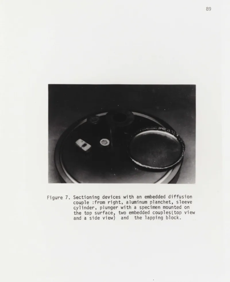
7. Sectioning devices with an embedded diffusion 89 couple

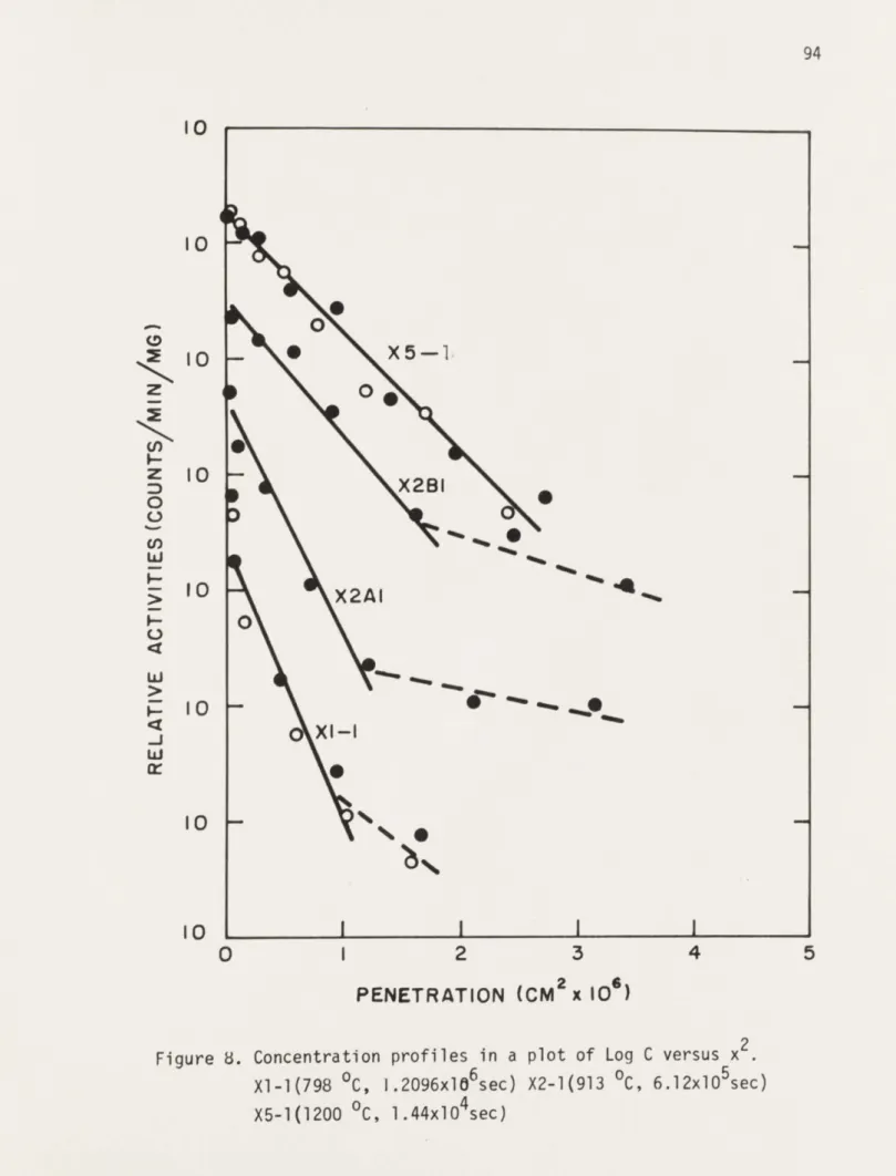
8. Concentrgtion profile in a plot of Log C 94 versus x for specimens Xl-l,X2-1,X5-1

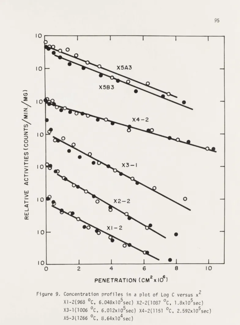
9. Concentration profiles in a plot of Log C 95 versus x2 for specimens X1.2, X2-2, X3-1

X4-2, X5-3

10. Concentration profiles in a plot of Log C 96 versus x2 for specimens Z6-2,Z6Al,Z8-l,Z5-2

11. Concentrgtion profiles in a plot of Log C 97 versus x for specimens Z4-1,Z5-l,ZlO-3

12. Concentration profiles in a plot of Log C 98 versus x2 for specimens Zl-l, Z6-3,Z5A3

13. Temperature dependence of cation self- 107 diffusion coefficients in single crystal ZnO

14. Concentrgtion profiles in a plot of Log C 111 versus x

Number Title

15. Concentration profiles in a plot of Log C 112

versus x

16. Concentr t on profiles in a plot of Log C 113

versus

x-17. Temperature dependence of cation dislocation- 118 pipe diffusion coefficients in ZnO

18. (A) C vs. r curves for various values of 6 121 (B) R~Tation between and systematic error

of apparant D due to grain boundary diffusion 19. Expected concentration profiles near a 123

termination point of a high diffusivity path ( schematic)

20. Concentration profiles of specimen P3A 126 in various plots

21. Concentration profiles gor various diffusion 127 annealing times at 954 C

22. Concentration profiles for various diffusion 128 annealing times at 1,123 OC

23. Annealing time dependence of grain-boundary 131 and apparant volume diffusion coefficients in ZnO 24. Temperature dependence of cation self-. 134

diffusion coefficients as obtained by various workers

25. An ideal hexagonal close-packed structure 145 with tetrahedral and octahedral interstitial

26. The crystal structure of zinc oxide shown 147 as a linkage of tetrahedraand octahedra

A-II-l. Micrographs of the basal plane after etching 201

in a boiling NaOH solution

A-II-2. Micrographs obtained after etching in 30 % 202 hydrofluosilisic acid

A-II-3. Micrographs of the oxygen surface after etch- 203 ing in 30 % hydrofluosilisic acid

x

Number Title Page

A-II-4. Micrographs of the second order prism plane 204 after etching in 30 % hydrofluosilisic acid

A-II-5. Micrographs of the basal planes obtained by 205 a thermal etch at about 1000 0_{C for three days}

A-II-6. Micrograph of a prismatic pit on the first 206 order prism plane

A-II-7. Micrographs of dislocation etch pits on basal 207 plane

A-II-8. Micrographs of etching morphology on the 208 second order prism plane (slightly-off)

A-III-l. Vacuum evaporation system 209

A-IV-l. The plateau curves of the proportional counter 216 A-IV-2. The proportionality between counting rate 217

Number Title Page

1. _{Cation self-diffusion in ZnO 39}

2. _{Oxygen and impurity diffusion in ZnO 61} 3. _{Cation self-diffusion coefficients along 105}

the a-axis

4. _{Cation self-diffusion coefficients along 106} the c-axis

5. _{Dislocation pipe-diffusion coefficients 116} along the a-axis

6. _{Dislocation pipe-diffusion coefficients 117} along the c-axis

7. _{Grain boundary diffusion coefficients at 129} T = 954 0C

8. _{Grain boundary diffusion coefficients at 130} T = 1,123 0C

9. _{Possible branches of diffusion jumps 149} 10. _{Diffusion coefficients through high 160}

xii

ACKNOWLEDGEMENTS

I am greatly indebted to Professor Bernhardt J. Wuensch, my thesis adviser. Without his able guidance and inspiration during the entire process of this work, from the suggestion of the problem to the correction of my faulty usage of English, this work Could not have been possible. I wish the pleasant memory of my adviser to last the rest of my life along with the highest form of training which he provided.

Professors W. D. Kingery and P. L. deBruyn are thanked for giving me the invaluable opportunity of graduate study at M.I.T. It is also a pleasure to acknowledge the learning from Professors R. L. Coble and D. R. Uhlmann.

I especially thank Professor K. C. Russell for allowing me to use his diffusion furnaces and vacuum evaporation system.

The personnel of the Ceramics Division have given constant stimulation and encouragement. The assistance of all the Ceramics staff is appreciated. The skillful drawing of Mr. Donald Fellows is greatly acknowledged.

My special thanks go to Dr. H. S. Choi, who introduced me to the exciting field of materials science. I am indebted to my parents, Mr. and Mrs. Minyul Kim, who have sacrificed themselves for all their children to have the highest education available.

My deepest appreciation goes to my wife, Hwasoo, not only for her moral support throughout the study, but also for her typing of the thesis patiently and the preparation of the manuscript.

This work has been supported by the U. S. Atomic Energy Commission under Contract Number AT(30-1)-3773.

I

I. INTRODUCTION

There are two important reasons for studying diffusion in solids. First, the kinetics of many solid state reactions are controlled by the rate of diffusion of one or several atomic species. The knowledge of diffusion is, therefore, essential in real understandings of kinetic problems such as phase transformations, precipitation, sintering, grain growth, recrystallization, annealing, homogenization, oxidation, creep and so on. The second reason for studying diffusion is to

understand more about atom movements and point defects in solids. Diffusion experiments have been the most frequently used means of studying defects, since the concentration and mobility of such defect can be theoretically related to the diffusion coefficient. More recently, investigators have been concerned with diffusion along potential fast diffusivity paths (dislocations and grain boundaries). It is frequently observed that the diffusivity along those paths is much higher than that of a tracer atom.in the lattice. The higher diffusivity is of great interest because there is the question of how and how much these high diffusivity paths contribute to the measured values of the diffusion coefficient. Quantitative knowledge of this enhanced diffusion may give important

such as precipitation, segregation and the annealing of

quenched-in vacancies along dislocations and grain boundaries. For instance, in ionic crystals there is increasing evidence

that the effective radius or width of the high diffusivity path is in the micron range rather than the few interatomic distances which had been assumed. Impurity segregation and precipitation or space charge could account for these wide regions of high defect concentrations.

It is, therefore, necessary to understand not only volume diffusion, but also the origin and magnitude of fast diffusivity in order to predict the circumstances where one of those diffusion mechanisms may be the dominant means of mass transport.

J II. THEORY

A. THE PHENOMENOLOGICAL DIFFUSION EQUATION

In the classical treatment of diffusion theory, it is assumed that the solid is a continuum. The detailed atomic structure of the solid is ignored. Although this approach has the obvious

disadvantage that the model does not incorporate any information on the mechanism of atom movement, it applies quite generally and shows what can be expected on a macroscopic scale.

The phenomenological formalism was early recognized by Adolf Fick1, who wrote the diffusion equation as

(II.A.1) J = -DV C

, where J is the flux of diffusing substance, C concentration and D the diffusion coefficient. When matter is conserved the flux equation leads to a continuity equation; the so-called " Fick's second law ":

(II.A.2)

_vJ

Further, if the diffusion coefficient D does not depend on

composition and hence on position, the equation (II.A.2) leads to a more convenient form

(II.A.3) _C

the equation (II.A.3) becomes the Laplace equation which appears

2 3

in a heat flow2 or potential field problem

In more general cases, however, the equation (II.A.1) is not adequate since the flux J and the concentration gradient -VC are not always parallel and a given component of the flux must therefore be related to each component of the gradient. ( Strictly speaking, driving force of diffusion is a gradient of chemical potential, not concentration. This becomes especially important

in ternary systems. ). Thus the equation must be written as

(II.A.4) J = - D V C i,j,= 1,2,3.

In this way the diffusion coefficient Dii is defined as a second order tensor which consists of nine elements. Fortunately the number of tensor elements may be reduced to a smaller number of independent element from the properties of second order tensors and further from the crystal symmetry. Without any assumption of an atomic process involved in the diffusion, it can easily be shown4 that, depending on the crystal symmetry, the coefficients can be represented as below, when the tensor is referred to a cartesian coordinate system oriented appropriately with respect to the crystallographic axis.

cubic D1 0 0 tetragonal D1 0 0

0 Dl 0 hexagonal 0 D 0

5 orthorhombic _-D 0 0 monoclinic _{D 0 D3 1}

1

Many interesting physical implications can be deduced from the above diffusion coefficient tensors. For instance, in a hexagonal crystal, the second order tensor quadratic equation can be written as

(II.A.5) D( y, Y2, Y₃) =D y 2 + D Y22 + D3 32

where Yi's are the direction cosines of diffusion directions with respect to the cartesian coordinate system. Now if the three fold or the six fold rotation axis ( the axis of the highest symmetry and the crystallographic c-axis ) of the crystal is chosen as the z-axis, the diffusion coefficient along a direction which makes an angle 0 with the z-axis will be

(II.A.6) D(0 )=DI sin®2 + D3 cos20

2 2 .2

since Y, + Y2 = sin 0

Now it is seen from (II.A.6) that along the z-axis ( when 0 =00), the diffusion coefficient is D3, while along the perpendicular to the z-axis ( _{E= 900), the diffusion coefficient is Dl.}

Furthermore they are extremal values, since it is always true that

multi-component systems, but also irreversible thermodynamics, where any constituent such as electron, hole, vacancy or

interstitial, is considered as an independent substance under the influence of general forces; an electrical field, a

temperature gradient and a chemical potential etc. In the generalized treatment, a flux can be written simply as

(IIA.7 ik L kI XI

( . 7J L X

j

where Jk=the flux of substance k, along the i-direction

I

X =the generalized force along the j-direction applied to 1-substance

Lk

_ii

It has been demonstrated that the theory together with the Onsager relationship5 leads easily to the well-known Darken equation 6, thermal diffusion , and solid electrolysis 8, as well as the diffusion of various defects9.

7 B. SOLUTIONS OF DIFFUSION EQUATION

Methods for obtaining diffusion coefficient from experiments are suggested by solving equation (II.A.3) under suitable boundary conditions!0 More complex cases such as moving boundaries are impractical, if not impossible, for use in experiments even though analytical solutions are often available in the literature.

B.l .VOLUME DIFFUSION

B.1.1 Sandwich couple

Perhaps the simplest solution with experimentally realizable boundary condition is the one-dimentional case in which a thin film of tracer is initially located in a layer of thickness 5

between two slabs of large surface area. The diffusion equation is then

-a

C

C

X.,t)

_C

₎

at

D

The boundary conditions are

C(x,t)=O when t=O forlxI/'2 (II.B.2) C(x,t)=cowhen t=u for x=O

00

The solution is

The diffusion coefficient then may be obtained from the slope of -1/4Dt provided by a plot of Log C as a fuction of x2 after a diffusion anneal of duration t.

B.l.2. Vapor exchange couple

In the case where a crystal is exposed to a constant concentration of diffusant, the boundary condition will be

for t!O C(x,t)=C at x=O (II.B.4) for t=O C(x,t)=C at x=O C(x,t)=O at x>O

The solution is

(II.B.5) _{;t 2 2}

_T~

where

e

c

=

-X-The diffusion coefficient may be evaluated from the slope of 1/1~4Dt provided by a plot of erfc (c ) as a function of

0

9 B.l.3. Three dimensional specimens

In many studies, the diffusion coefficient has been obtained from a vapor exchange with all surface of a small crystal. In this case separation of variables provides a powerful means of solving the equation.

(II.B.6)

Experimentally realizable boundary conditions are:

C=C0 C=Cg

at t- O at the interface at t=O inside the crystal The solutions1l depend on the geometry of the sample.

(i) A slab of thickness 1

-D(2'T+lfYt/ 4 z +r

2).

00

Mt

0-Bo7

C- C;_ 20* =

I-CO

-C'ZLI

-P

e

e-'Ddt T

(-d.,)

e

w

where d-.,'s are the positive roots of J0 (c6&)=O and J₀ represents the first order Bessel function.

The total amount diffused out or into the sample is

Mt+

e-

t

a..

C - C;.*

C -C;

Mt

,where M=the total amount in equilibrium(after long time) Mt=the total amount at time t

As the equations imply, the diffusion coefficient cannot be obtained in a straight-forward fashion as in the above two simpler cases. However, in most cases the first terms of the series usually suffice to give fairly good approximations for solutions if suitable experimental conditions are chosen. It is then possible to caculate the diffusion coefficient. For instance, for long

time annealing the average concentration C C &-. can be represented by a simple form12

(II.B.7)=A

-- C,

where C, Cf and C i are average, initial and final concentrations A a constant depending on a geometry and ' "relaxation time" which depends on the geometry as follows:

I1 geometry relaxation time (t)

Slab

'71'D

Cylinder _2.0;,

Sphere ebraD

, where h is the thickness of slab and a the radius of cylinder or sphere

r-Cf

From a plot of Log f as a function of t, the diffusion 1- f

coefficient may be obtained from the slope of /t

B.2. ANISOTROPIC DIFFUSION

Basically the diffusion equation of an anisotropic crystal has the same solution as that of an isotropic crystal. From the general flux equation (II.A.4)

9

C

(II.B.8s)

D

C

V-=.902-

_C

under the conditions that matter is conserved ( there is no sink or source ) and D. 's are independent of the concentration. Since it can always be shown that D .V. C=U, when itj from either a second order tensor property 13 ( 0i= Dj ) or the Onsager relation5 ( Dii = -D.), the equation (II.B.8) becomes

ac

,where Dii's are the diffusion coefficients along the three principal axes. What equation (II.B9) means is that the D

component can be obtained simply by measuring the property along the principal axis i in the same way as in an isotropic crystal.

B.3. GRAIN BOUNDARY DIFFUSION

An exact model of grain boundary diffusion is yet to be formulated. Numerous approximate solutions have been applied to obtain grain boundary diffusion coefficients.

Fisher14 derived the first analytical expression for concentration as a function of penetration when grain boundary diffusion occured simultaneously with volume diffusion. He assumed that the grain boundary could be imagined as a slab of uniform width 9 with a uniform difffusivity Db which extended to infinity in the y-z plane of a crystal ( Figure 1. ). He then set-up two differntial equations; one inside of grain boundary region, the other outside the grain boundary.

Region (I)=outside the boundary

ac

a'

jc

13 Region(II)=inside the boundary

?C -

.

The boundary conditions were taken to be those of the vapor exchange couple (II.B.4), i.e., a constant concentration at the surface.

-a C aCj

Under assumption that Dbl)m l - =0, ' =small for large penetration distance, he solved the simultaneous equations (II.B.10) and (II.B.11) to obtain the concentration profile;

(II.B.12) tpC %F -k X

bZ/DC

(-YDt)

2

Thus SDbmay be obtained from the slope of a plot of ln C as a function of y at large penetration distance (for any x). Further

the slope of (II.B.12) was shown not to be changed markedly even in a polycrystal with many high diffusivity palnes, provided that the distances between them were greater than about V4D7t.

Whipple1 5 and later Milford and Maneri1 6 solved the equations (II.B.10) and (II.B.11) with more realistic boundary conditions at the interface of two regions:

(II.B.13)

a C -a~ e 'if'

0

F

an expected

concentration

proti Le

8 (G.B. width)

Figure 1. Co-ordinate system for analysis of dual-kinetics diffusion

h

15

where CI and C are concentrations in region (I) and (II) respectively. Introducing new variables

(LI.B.14)

,

/

-Dit

AT

Whipple solved the equations for the concentration profile:

_ _

1

a

Notice that the first term in (II.B.15) is same as the solution of volume diffusion for a vapor exchange couple; i.e., equation (II.B.5). The final expression was numerically evaluated as a function of I and V, in the neighborhood of the grain boundary. Since the concentration profile may be experimentally obtained, the value may be computed by comparing the experimental contour with an iso-concentration contour of the numerical solution.

The analysis by Fisher and Whipple employed the boundary condition of a constant concentration. The solution for the boundary condition of a finite concentraion ( or "instantaneous

17c18

With the "instantaneous source conditions" ac

(g)

0

=o;

0

(

&v

(II.B.16)

C (x ,O, t)=,

C(Oo

,t)=0

Suzuoka solved the simaultaneous equations (II.B.10) and (II.B.11) with the additional boundary conditions (II.B.13) to give the

concentration (II.B.17) A 2 + D%?(-Z)Jt4C [[&-i t 6- 1 d6l Z__ _il -]

47-CD

_tr

%t.

_{a, -}

Td-Notice again that the first term of (II.B.17) shows the

contribution by volume diffusion of the thin film solution (II.B.3). The practical applicability of equation (II.B.17) results when the average concentration is computed. Including the effect of grain size,

(II.B. 18)

%t),

,) k

-F

4

where n= grain size parameter = (grain size)/14pgt

)=6(1)

C (-X,

_P

_{- ) -}

_{I ---}

_{:. ^P}

17

VAAC

Typical concentration profiles calculated from (II.B.18) are given in Figure 2. _{By numerical calculation it was found that in C}

H was very closely proportional to the 6/5 power of the penetration

depth. The result was conveniently represented by a relation

(II.B.19) -

o3

(II.B.19) was valid within an error of less than 5 percent in a range of about 1 to 100. At a large penetration depth, where there is practically no contribution by volume diffusion, in Cl can be substituted by In C without any significant error. Further it was found that the result was very insensitive to n, although n was a function of The lower limits of validity for such substitution were nt3.5 for P=I n 2.5 for =0.01, a

condition satisfied in most experiments, Thus the value may be obtained from the slope of a plot of In T versus y6/5

All the analyses by Fisher, Whipple and Suzuoka assumed a small boundary width S . Recently Mimkes and Wuttig19,20

solved the problem considering a finite thickness of & . They found that outside grain boundary region, the Suzuoka analysis

0

13=1

gf3=100

0

2

4

6

8

10

12

Figure 2. Penetration curves Cs(z)=exp(-z2" /4) + C₁₁(z) for n=10.

The dashed straight line for p=4 shows the grain boundary diffusion supposed on the basis of Fisher's

solution. [After Suzuoka(17)] Arrows mark the observable ranges of contribution by grain boundary diffusion.

19 was a good approximation for small 6 , but for a larger a , the concentration profile may be considerably different, because the amount of diffusant present in the grain boundary region can no

longer be neglected. Unfortunately the Nimkes and Wuttig analysis did not provide a simple way to obtain dislocation or grain boundary diffusion coefficients. Every concentration profile must be fitted by a trial and error procedure.

C. RANDOM WALKS

The formal relation between random walk and macroscopic

21

diffusion phenomena was first derived by Einstein2. He derived the equation

(II.C.1) B = kTD

where B=mobility of particle k=Boltzman constant D=diffusion coefficient

In the general theory of random walk, the position R of a particle displacement is given by

(II.C.2) R = r i=1,2, '' n

where ri's denote the different displacements. The probability WN (R)dR that the position of particle after N steps is located

in the interval R to R+dR, which is eventually related to the diffusion, can be found by various methods22. In this study a

method derived by S. Chandraskhar23 and applied later by Manning24 will be followed to understand the principal feature of the

relationship.

C.l. ONE DIMENSIONAL RANDOM WALK

Suppose a particle moves along a straight line in a series of steps of equal length 6L . Either forward or backward jumps

21 may be made and each has an equal probability 1/2. Let the duration of step be t7 . After taking N steps, the particle could be at any one of the points -N, -N+l, .... ,-2,-l,0,l,2,....,N-l, N.

Let W(mok; ZN)=W(m;N) be the probability that the particle will arrive at m after N steps after having started from an origin 0. In order for a particle to arrive at m among N steps, some (N+M)/2 steps should have been taken in the positive direction and the remaining (N-M)/2 steps in the negative direction. Since the probability that the particle will take the Nth step in a definite direction, say towards to the m position, is (1/2)N, the probability

W(m;N) will be

(II.C.3) W( 'N

Since the case of the greatest interest arises when N>"> m, the equation (II.C.3) can be simplified by Stirling's formula and by series expansion to provide

(II.C.4)

_(em;

₎

=2

Now it is desirable to find the formal relationship between discrete random walks and a continous diffusion equation. From the equation

(I I. C.5) W ('M-N)= ! (" -. ; N)+IW ('M+\ ' N)

The equation (II.C.5) can be re-written in the equivalent form:

W (m; N+ )-W (n ; N)

(II .C.6)

I

(?+1 N)-2_W(m;

_{N) +U~-l}

_(e

₎

after division of both sides by ' and

Now suppose that CL and t approach zero in such a way that

(II.C.7)

Nt

=t

Then equation (II.C.6) becomes in this limit, recalling W(m,N) = W(mo(;NZ: ),

(II.C.8)

Wt

,which is in a form similar to the diffusion equation (II.B.1) in one-dimension. Further, the equation (II.C.4) may be written in

Using the relationship

2

t

=

23

(II.C.9) W(x,N)AX = W(m,N) Am

,where the factor two comes from the fact that m can take only even or odd values depending on whether N is even or odd in deriving

(II.C.3), together with & x = oc- a m and equation (II.C.7),

(

The probability W(x,t) A x that the particle will find itself between x and x+Ax after time t is

(II.C.1I)

2(7cpt)

tx

P

4-Z

*)'

Now writing = T , where T is the number of displacements per unit time, the diffusion coefficient is given by

(II.C.12) :b $ = .7

Finally, when the fundamental assumption is accepted that the probability of a particle movement is same as the average movement of large number of particles, equation (II.C.8) becomes Fick's

second law (II.B.1) and one of its solutions is the thin film

2-N) Ax

₎

-solution

(II.C. 13)

C

(xt

L.)

The above derivation is not mathematically rigorous. However, it shows how the random walk problem is related to a diffusion process.

C.2. THREE DIMENSIONAL WALK, DIFFERENT JUMP DISTANCES

Assuming the random walks to be independent of the directions, the probability W(M:N) at a three dimensional position M from an origin is given by

(II.C. 14) W(M:N)=W_{1 (m ;N}

1) W2(m2;N2) W3(m3;N3)

,where W.(m.;Ni) is the probability that the particle will be present at the position m. on the i-axis. Then for each W. (m.;N.), the equations (II.C.3) and (II.C.11) will hold. Thus

(II.C.15) r t)..

TJ[*D,'D~ff* \4At4pat4t)

,where

( II.C.16) D = 1 C %

25

Further analysis may be continued for the cases where more than one jump distance is encountered. Suppose the probability that a particle suffers N₁ random jumps of distance d₁,and N₂ Of 0.

to arrive at the position x in one dimension. The net displacement is given by m, 0C, +m20"-= x, + x2 = x. The

probability to arrive at x1 , W1(x1 ;N1 ) A x is followed by

the probability W2(x2;N2) Ax2 which will lead to the final

position x. Then the probability that the particle will arrive at x after N₁ and N₂ steps is

(II.C.17)

_{W (X; N, N}

₎₌

_)~W2

_(a)A

2

, Nt,

₂

Now using the facts that

x₂ = x - x ₁ and dx2 =dx

(II.C.18) 00

After substituting (II.C.10), the integral (II.C.18) can be performed exactly to yield

(II.C.19)

The diffusion coefficient is

D -

₂

_-

₂

I

₁

+L - -+

_IF2

(II.C.20)

The same analysis may be repeated in case of many jump distances with the result

(II.C.21)

In many situations which arise in a crystal, the magnitude of the jump distance C. will be same but the directions could make different angles 9Z with respect to a reference axis. In those cases it can be readily seen from the equation (II.C.21) that the diffusion coefficient is given by

(I I C.22) 2

2ZUc~~G

Provided that is the same, the problem will be the evaluation

of

C-.o

s

osG

so-called "correlation factor" and the subject of further discussion.

27 C.3. EXAMPLES

C.3.1.Cubic structure

(i) Simple cubic

(ii) Body centered cubic

D [4

4()1Vf

(iii) Face centered cubic

,where

F,

_r

(

_(-.-)

Sare jump frequencies along the edge,

face diagonal and body diagonal respectively. C.3.2. Hexagonal structure

In a hexagonal structure, there are two kinds of jumps; one on the same basal plane

Fa.

Along the c-axis

D~-~j3F

Along the a-axis

1"2,(-

_)]

_=-

_[3F

_4n

_]

+

i>) + 2.1F (09

0

F,

_{+ 6F}

C1

b

00 +

D=-L.2

2=

[4G

D. CALCULATION OF DIFFUSION COEFFICIENT

The equation (II.C.21) gives in principle a way to calculate a diffusion coefficient. Since the jump distance o(, can be

well-defined for a crystal, the problem is to calculate the jump frequency

f.

Literally, the quantity

F

(II.D.1)

T

=

_\cw

The proper values of N and co depend upon the atom movement and its enviroment: that is, they are functions of a diffusion mechanism. Before discussing the quantities N andco , it seems

however proper at this point to mention briefly the "correlation effect" in diffusion.

D.l. CORRELATION EFFECTS

In deriving the equation (II.C.21), it is assumed that the successive jump directions of an atom are not correlated. However, this is not generally true, especially for diffusion of a tracer. The tracer atom will be more likely to jump backward to the initial position. Thus the tracer jumps are correlated.

29 As a first approximation, the correlation factor f can be represented for a vacancy mechanism25 by

(II.D.2) f = 1 2

z

where z is the number of nearest neighbors.

A rigorous calculation by Compaan and Haven26 shows that for tracer diffusion by

a vacancy mechanism

(II.D.2a) I t 4 cIOS G> J - < Cos 0>

an interstitialcy mechanism

(II.D. 2b) J = 1 4- <COS 19'>

,where <U0s> is the average of the cosines of jump directions which appeared in (II.C.22) and calculated for various crystal

lattices.

Being directly related to a diffusion mechanism, the

27

correlation factor has been used to elucidate the mechanism In alkali-halide crystals, the correlation factor can be readily obtained by comparing the tracer diffusion coefficient and the ionic conductivity. Those two quantities are related by Nernst-Einstein relationship28_.

O' Nh

(II.D.3) =

=r

,where d'= ionic conductivity T=temperature

D=Diffusion coefficient q=charge of particle k=Boltzman constant N=concentration

In principle, the same analysis may be applied to oxides. In practise, however, only questionable results are obtained for most oxides because of difficulty in measuring accurately the diffusion coefficient, and because electronic processes may contribute to the conductivity.

D.2. THE JUMP PROBABILITY CQ .

The quantity W' , the probability for the jump of an atom into an adjacent site, is the least known of the terms which enter in

the calculation of the diffusion coefficient. There have been many approaches to this difficult problem: the random probability

fluctuation of a particle to escape over a potential barrier29 in terms of "activated complexegfrom the absolute reaction theory 30; by calculation of equilibrium partition functions 31

the distribution of actual vibration modes of an atom32,33 and 34-36

31

The results reduce in all cases to a simple form

(I I. D.4) _Co

₌

,where = the vibrational frequency of an atom about its equilibrium site ( usually taken to be the Debye frequency).

A gm = the free energy of motion36'37

The present knowledge of this quantity o is limited to this point. Further work must be done in order to enhance our

understanding of diffusion.

D.3. THE DEFECT CONCENTRATION N.

In comparison with W) , the equilibrium concentration of defects N is a quantity which is better understood. The

thermodynamics of defect chemistry38 provides the means for

calculation of the concentration in terms of equilibrium constants. A compound MX can have many defects; cation vacancies VM9 anion vacancies VX, cation interstitials M1 , anion interstitials

Xi, ionized states of those defects, as well as electrons(e) and holes(h). Fortunately, in many cases, one of two types of defects may predominate in a crystal; either Schottky defects ( VM and VX)

A simple method for calculation of the defect concentration is to find the pseudo-chemical equations of defects. For example for a Frenkel defect

(II.D.5) 0 4;=

ML

V,

Vm] =

where A gf = the formation energy of a Frenkel pair

[Mi],[VM] = the mole fractions of the cation interstitial and vacancy respectively

For an ideally pure crystal [VM] = [Mg], so that the defect concentration will be

(II.D.6)

N

=

M

j

=

Vm1

= e

2T

One very interesting case typically occurs in a crystal which contains a cation impurity of different valence. In this situation in order to maintain the charge neutrality of the crystal, one of defects may increase or decrease its concentration. Suppose, for example, XI and X2 are two complementary defects (M₁ and VM for a Frenkel defect, VM and VX for a Schottky defect), then

(II.D.7) 0 = X + [X 1[X2 = exp(- kT )

33 Assuming that the impurity C acts to increase X1, then to

maintain charge neutrality

(II.D.8) _{X = C + X2}

Substituting equation for X,

(II.D.9)

C

(II.D.8) into (II.D.7) and solving the quadratic

II

I

1

ArC4 i

This formula expresses the change of defect concentration as a function of temperature.

If C2 T

[X,) TC1-

C

If C2 <-4

(

Two limiting cases are of interset.

high impurity concentration or temperature)

low

low impurity concentration or high temperature)

-e

A

The two ranges are the so-called "extrinsic"

ranges, respectively. The significance of the result will discussed later in connection with the diffusion coefficient of

a crystal.

and "intrinsic" be [-XII

=U10

atmosphere on defect concentrations. Suppose that an atom M is incorporated in a crystal MX by formation of a singly ionized interstitial. Then M(g) = M. + e MX = M(g) + I X₂(g) K1 = n _MM ] 1/2 K_{2 c M P} X₂

Now if all electrons originate from Mi, then the charge neutrality is

(II.D.13) [ M] = n

From (II.D.ll), (II.D.12) and (II.D.13), it is seen that the defect concentration is a function of gas pressure;

IM0.

I

C,

2

-

A

0

The above examples are rather simple cases. To be rigorous, several kinds of defects should be included with a suitable charge neutrality condition.

(II.D.1l)

and

(II.D.12)

35

D.4. DIFFUSION COEFFICIENTS

It is now possible to express the diffusion coefficient more explicitly. For example, in a cubic crystal . from

(II.C.23)

(II.D.15) D = fa2 = fN a2

For a vacancy mechanism N will be same as the mole fraction of vacancies NV so that D = f a2 N C%) . When a solute in a dilute solution diffuses by an interstitial mechanism, D = a2c W , since the mole fraction of vacant site is essentially unity.

An elegant way to interpretlthe diffusion mechanism is found through the effects of impurity and the environmental atmosphere. First, if a crystal with a Schottky pair has a divalent cation

impurity, the diffusion coefficient will be from (II.D.3), (II.D.10) and (II.D,15),

(II.D.16)

-

Slope =Ah/2

#Ahm

Slope

=Ahm

Slope =Ah/ 2+

Am

---

Slope =

&'m

1IT

-A typical plot of diffusion coefficient as a

function of inverse temperature for cation diffusion (upper line) and anion diffusion(lower line), when an aliovalent impurity atom creates a cation vacancy.

Ah= Formation energy of a Schottky pair.

h mh' = migration energies of cation and anion respectively.

0

-J

37

,where asm and A ss are entropies of the migration and the formation of Schottky pair respectively. Thus a plot of Log D

as a function of l/T would exhibit a break at a low temperature as indicated in Figure 3. At the temperatures above the "knee" the diffusion coefficient would be same as that of ideally pure crystal. Below the "knee" it would be controlled by impurities.

Similarily, when a singly ionized interstitial cation is formed due to the gas atmosphere, as seen in (II.D.13), the diffusion coefficient would be

. -1/4 1/2

(II.D.18) _{Doc. [ M ] aC PX2}

or cc PM

Thus when diffusion coefficients are measured as a function of a gas pressure, a diffusion mechanism can often be elucidated from the exponent of the pressure dependence.

III. LITERATURE REVIEW

39

Because of a vast amount of work on diffusion, as well as a periodic publication to review recent datal0 this review will be limited to diffusion in zinc oxide and works related to its defect structure. Anisotropy of diffusion coefficients is one of main concerns of this study, so that results on simple non-cubic oxides will also be included.

A. CATION SELF-DIFFUSION IN ZINC OXIDE

Beginning with Wager's4 interpretation of the parabolic tarnishing reaction of metal zinc in terms of interstitial zinc diffusion, cation self-diffusion in zinc oxide has been a subject of many studies. A considerable amount of work and discussion has also appeared in connection with the diffusion experiments. Under certain assumptions the diffusion coefficient can also be calculated from electrical conductivity measurements, oxidation kinetics

and sintering experiments.

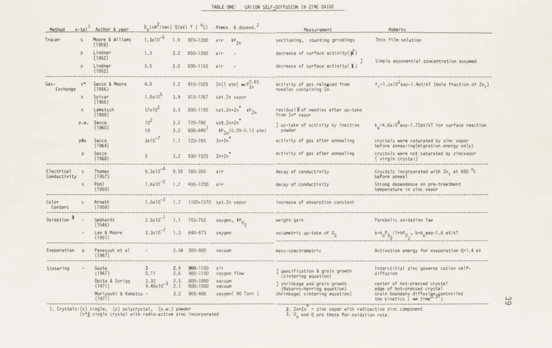
For the sake of convenience in our discussion the results are summarized in Table one and will be reviewed from the

TABLE ONE: CAIION SELF-DIFFUSION IN ZINC OXIDE

Method x-talI Author & year D₀ (cm2/sec) Q(eV) T ( 0C) Atmos. & depend.2 Measurement Remarks

Tracer s Moore & Willams 1.3x10-5

1.9 970-1200 air PZn sectioning, counting grindings Thin film solution

(1959)

p Lindner 1.3 3.2 850-1200 air - decrease of surface activity(p+c

] Simple exponential concentration assumed

p Lindner 3.5 3.0 800-1150 air - decrease of surface activity(1)

(1952)

Gas- s* Secco & Moore 4.8 3.2 910-1025 Zn(l atm) %cP0.65 activity of gas released from f.=l.zxl02exp-1.4eV/kT (mole fraction of Zni)

Exchange (1956) Zn needles containing Zn;

s Spicar l.8x105 3.9 910-1267 sat.Zn vapor

(1956)

s Lamatsch 1.7x102

3.3 800-1190 sat.Zn+Zn* *P residuallof needles after up-take

(1959) from Zn* vapor

p.w. Secco 102 3.2 720-780 sat.Zn+Zn ] up-take of activity by inactive k =4.6xi04exp-1.72eV/kT tor surface reaction

(1960) 10 3.2 800-840 _{4PZn(0.09-0.13} atm) powder e

p&s Secco 3x10~7 1.1 720-760 Zn+Zn* activity of gas after annealing crystals were saturated by zinc vapor

(1964) before annealing(migration energy only)

p Secco 5 3.2 930-1025 Zn+Zn* activity of gas after annealing crystals were not saturated by zincvapor

(1968) ( virgin crystal)

Electrical s Thomas 5.3x10-4 0.55 180-350 air decay of conductivity Crystals incorporated with Zn at 650 0C

Conductivity (1957) before anneal

s Pohl 1.6x10-2 1.7 400-1200 air decay of conductivity Strong dependence on pre-treatment

(1959) temperature in zinc vapor

Color s Arneth 1.5x10-2 1.7 1100-1370 sat.Zn vapor increase of absorption constant Centers (1959)

Oxidation ₃ - Gebhardt 2.5x10 7 1.1 703-752 oxygen, P₀ weight gain Parabolic oxidation law

(1946) 2

- Lee & Moore 3.3x10 7 1.3 648-673 oxygen volumetric up-take of 02 k=ko P /l+bP₀ , bzb0exp-1.8 eV/kT

(1951) 02 0

Evaporation p Panasyuk et al - 2.04 300-800 vacuum mass-spectrometric Activation energy for evaporation Q=1.4 eV

(1967)

Sintering - Gupta 3 2.9 900-1100 air Interstitial zinc governs cation

self-(1967) 0.11 2.6 900-1100 oxygen flow ( dning q ain growth diffusion

Dutta & Sprigg ₍₁₉₇₁₎ 2.32 _9.48x10 -3 2.5 800-1000 vacuum ] shrinkage and grain growth center of hot-pressed crystal 2.1 800-1000 vacuum (Nabarro-Herring equation) edge of hot-pressed crystal Moriyoshi & Komatsu - 3.2 905-800 oxygen( 80 Torr ) Shrinkage( sintering equation) Grain boundary diffusi n3 ontrolled

(1971) the kinetics ( ca time ) (A3

1. Crystals:(s) single, (p) polycrystal, (p.w.) powder 2. Zn+Zn = zinc vapor with radioactive zinc component

A.I. TRACER DIFFUSION AND GAS EXCHANGE

A.I.I. Single crystals

Despite much works on zinc oxideexperiments with single crystals are very rare. The reason is simply that it is extremely difficult to grow large crystals of good quality: zinc oxide

sublimates before melting.42 However, considerable progress has been made recently.43 All previous works were confined to

studies of small needles with a diameter of less than one millimeter.

The work by MLnnich44 and the unpublished work by Spicar 45

were two early works by gas exchange methods on single crystal needles.

Secco and Moore4 6 used a large number of single crystal

needles into which radio-active zinc-65 had been incorporated during the crystal growth. The measurement of radioactivity in an initially inactive zinc atmosphere lead to an activation energy of diffusion of 3.17 eV at one atmosphere zinc pressure. The diffusion coefficient depended on zinc vapor pressure as

D oc PZn0.65 at 1,000 0C, which they considered to be reasonably

close to P0.5 _{. Since this value would be expected to be}

Zn

associated with singly charged zinc interstitials, they concluded that the diffusion process must be controlled by this defect. They alsomeasured the solubility of excess zinc by titration

41

with iodine. A heat of solution of excess zinc was found to be 1.39 eV from the measurement of mole fraction of excess zinc. Secco and Moore analyzed their data by assuming a diffusion controlled exchange rate. However the validity of this critical assumption was not rigorously proved.

A zinc vapor pressure dependevce was not observed in a similar work by Lamatch.47 He put crystals in saturated zinc vapor containing a radio-active zinc component. He measured the gamma activity taken up by the crystal by etching the crystal step by step. The activation energy, 3.3 eV, which was obtained is very close to the value obtained by Secco and Moore.46

But the different effect of the zinc vapor pressure in the two experiments is somewhat conflicting if the same kind of defect is pesponsible for the diffusion process.

To our best knowledge, the only work which employed

conventional sectioning of a single crystal to obtain the diffusion coefficient was done by Moore and Williams.48 They found an

activation energy of 1.9 eV for crystals annealed in air. They also cited the heat of solution of interstitial zinc as 0.15 eV in one atmosphere zinc vapor pressure for a certain zinc oxide powder. Since no significant zinc vapor pressure dependence of the diffusion coefficient was observed they concluded that the cation self-diffusion in zinc oxide was

primarily due to thermally genarated interstitial zinc rather than those due to departure from the ideal Zn/O. Thus they implied that the diffusion coefficients observed were in the intrinsic range.

It is general ly believed that diffusion data obtained by a sectioning technique are more reliable than those measured by a gas exchange method since it is not necessary to make major assumptions concerning the rate controlling step. The activation energy of 1.9 eV obtained by Moore and Williams48 is smaller by a factor of almost two compared to the values

Mor

47

obtained by Secco and Moore and Lamatsch . Nevertheless

Moore and Williams did not attempt in their paper to analyze the significance of the difference.

A.I.2. Polycrystals

Because of a possible contripution by grain boundary diffusion We must be careful to accept a volume diffusion coefficient obtained from a polycrystal. Nevertheless, many volume diffusion coefficients for zinc oxide were obtained

from studies on polycrystals, especially in early days. Lindner4 9 measured the cation self-diffusion of sintered zinc oxide tablets with densities 4.6-5.5 gm/cm3

43 air. He used two different experimental techniques:one by measuring the positron activity released from a radio-active thin film deposited on polycrystal; the other one by monitoring an up-take of gamma radioactivity of an initially inactive polycrystal in contact with a radio-active tablet. The

results were almost identical, and provided an activation energy of 3.2 eV.

The validity of Lindner's work depends on the assumption of a profile predicted by the simple volume diffusion equation. This might not have been true, because of grain boundary diffusion. However, Lindner's results can be favorable compared with a

subsequent series'of works by Secco.

In the first of a series of works, Secco50 measured the up-take of activity by initial ly inactive zinc oxide powder from radio-active zinc vapor. He analyzed his data by assuming that at the surface of a first-order reaction prevailed with an activation energy of 2.43 eV at a zinc vapor pressure of one atmosphere. This was followed by an auto-catalytic exchange process for which the evaporation rate was given by a rate constant ke = 4.6 x 104 exp ( -1.72 eV/kT ) sec~1

In this work, Secco attributed a strong zinc vapor pressure dependence of the rate to adsorption of zinc on the surface. The surface reaction was considered to be one of the rate

determining steps in the exchange reaction.

In a similar work,51 he did not observe a dependence of the rate on the zinc vapor pressure, at least up to 800 0C. He obtained two activation energies of 1.72 eV and 3. 02 eV for

the gas exchange rate in conjunction with two diffusion cosfficients which had same activation energies of 3.17 eV but different

pre-exponential factors. Re interpreted the smaller activation energy, 1.72eV, as one required to simply incorporate the tracer atom into the oxide and the larger one, 3.17 eV, as the activation energy for a direct movement of interstitial zinc between two

interstitial positions. In this work, however, the separation of data into the two diffusion coefficients seems to be poorly justified by his arguments. If we actually fit one straight

line through most of his data points ( Figure 7 of reference 51), the slope is found to correrpond to about 1.7 eV.

Secco reasoned in his later works 52,53 that cation

self-diffusion in zinc oxide might occur by a composite mechanism, perhaps by an interstitialcy mechanism. If this is the case, he argued, the activation energy of diffusion should be about 1.7 eV when measured at an equilibrium concentration of defects.

One of Secco's latest observations54 may be concordant with this interpretation. From similar gas exchange experimert

45 interstitial zinc, with an activation energy of 1.07 eV, and

another for an evaporation of interstitial zinc with an activation energy of 3.17 eV.

The activation energy of mobility 1.07 eV is a bit smaller than 1.7 eV Secco reasoned. Further the results are rather confusing if we notice that his results on polycrystals are almost identical to the result on single crystals.46 Since his works on polycrystals'were conducted at temperature ranges considerably lower ( up to 840 OC ) than the work on single crystals ( 910 0C-1,025 0C ), grain boundary diffusion could have been important in studies on polycrystals. It is , however, clear from the series of works by Secco that the surface reaction must be very important in the interpretation of a diffusion study of zinc oxide performed with the gas-exchange method.

At this point, the work by Roberts and Wheeler55'56 must be mentioned. They measured the diffusion coefficient

of sintered polycrystals with densities less than 93 % theoretical. Samples were annealed in oxygen and in argon in a temperature

range of 800 0C - 1,400 0_{C. They measured a decrease of residual} activity after having deposited a thin film 6n the surface of a crystal. Autoradiography with the residual activity in a polished specimen showed clearly that grain boundary diffusion

persisted at long depths into the specimen. They proposed that tracer penetration in most experiments on polycrystals was predominantly along grain boundaries at temperatures up to

at least 1,300 0C.

Assuming a simple exponential concentration profile inside of a crystal, Roberts and Wheeler analyzed their data according to the Fisher model14 and obtained a grain boundary diffusion coefficient

They also observed that Dat l, 90 0C. The penetration

6Db a

distance in a specimen annealed in argon was far greater than that in oxygen. From this observation they reasoned that perhaps Schottky defects may be more important in diffusion than

interstitial zinc, since the effect must be reversed due to increase 6f zinc interstitials in oxygen.

Unfortunately, grain growth was not controlled during

the diffusion annealing in Roberts and Wheeler's work ( by, for

example, firing the crystal at a higher temperature than the temperature at which the diffusion specimen was prepared). The results displayed a large amount of scatter, perhaps due to an excessive evaporation of the tracer and uncontrolled