Brief communication: Ad hoc estimation of glacier contributions to sea-level rise from the latest glaciological observations

Supplement of The Cryosphere, 14, 1043–1050, 2020 https://doi.org/10.5194/tc-14-1043-2020-supplement © Author(s) 2020. This work is distributed under the Creative Commons Attribution 4.0 License.

Supplement of

Brief communication: Ad hoc estimation of glacier contributions to

sea-level rise from the latest glaciological observations

Michael Zemp et al.

Correspondence to:Michael Zemp (michael.zemp@geo.uzh.ch)

2

Table S1 Overview on regional data availability and complementary data series from neighbouring regions. The table shows the overall number of glaciers with glaciological (glac) and geodetic (geod) observations as available in the reference dataset by Zemp et al. (2019, based on the FoG database version 2018-11) as well as available updates of the glaciological sample (all) and corresponding WGMS reference glacier sub-samples (ref) for 2016/17 and 2017/18 (based on the FoG database version 2019-12). Complementary mass-balance series from neighbouring regions were used for regional mass-change estimations in ad hoc years without glaciological observations. For

5

the present study, we excluded the glaciological data of Hamaguri Yuki, a perennial snow patch in Japan, region 10. Region Complementary mass-balance series Zemp et al.

(2019) glac / geod 2017 all glac 2017 ref glac 2018 all glac 2018 ref glac 01 Alaska Place, Helm, Peyto, Columbia 2057, Rainbow, South

Cascasde (all 02)

26 / 1,220 4 3 2 1

02 Western Canada & USA Gulkana, Wolverine, Lemon Creek (all 01) 55 / 95 14 6 9 2 03 Arctic Canada North Midtre Lovenbreen,

Austre Broeggerbreen (all 07)

17 / 6 4 4 0 0

04 Arctic Canada South White Glacier (03), Meighen Ice Cap (03), Devon Ice Cap NW (03), Melville South Ice Cap (03), Midtre Lovenbreen (07), Austre Broeggerbreen (07)

9 / 11 0 0 0 0

05 Greenland Storglaciaeren (08), Storbreen (08), White (03) 13 / 1,206 3 0 1 0

06 Iceland Storglaciaeren, Storbreen (08) 16 / 283 9 0 6 0

07 Svalbard & Jan Mayen Storglaciaeren, Engabreen, Langfjordjoek. (all 08) 21 / 1,110 10 2 7 2

08 Scandinavia none _{57 / 1,047 18 8 11 8}

09 Russian Arctic Midtre Lovenbreen, Austre Broeggerbreen (all 07)

3 / 373 0 0 0 0

10 North Asia Ts. Tuyuksu (13), Urumqi No. 1 (13) 19 / 11 0 0 0 0

11 Central Europe none 77 / 1,451 51 11 36 9

12 Caucasus & Middle East Argentiere, Saint Sorlin, Sarennes, Gries, Gietro, Allalin, Silvretta, Vernagt, Hintereis, Kesselwand, Careser (all 11)

12 / 362 2 1 2 1

13 Central Asia Leviy Aktru (10), Maliy Aktru (10), Vodopadniy No. 125 (10), Chhota Shigri (14), Hamtah (14), Parlung No. 94 (15), Mera (15)

42 / 4,314 12 2 11 2

14 South Asia West Ts. Tuyuksu, Urumqi No. 1 (all 13) 11 / 3,631 0 0 0 0 15 South Asia East Ts. Tuyuksu, Urumqi No. 1 (all 13) 21 / 1,182 6 0 3 0 16 Low Latitudes Echaurren Norte, Martial Este (all 17) _{14 / 49 7 0 5 0} 17 Southern Andes Yanamarey, Artesonraju, Zongo, Charquini Sur,

Antizana 15α, Conejeras (all 16)

14 / 2,331 9 1 7 0

18 New Zealand Echaurren Norte, Martial Este (all 17) 5 / 439 2 0 2 0 19 Antarctic & Subantarctic Echaurren Norte, Martial Este (all 17) 20 / 6 3 0 1 0

3

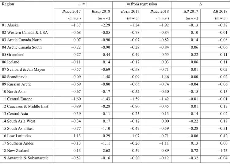
Table S2 Ad hoc estimates of regional mass changes for 2016/17 and 2017/18 according to different regression models.

Specific mass changes (B

) are shown for ad hoc estimates (Eq. 4) with slope m equal to 1 (as used in Table 1) and with m

as derived from linear regressions (as shown in Fig. S2), together with corresponding differences (ΔB) for both years. Large

values for ΔB are found in regions with small slopes and low correlation coefficients (e.g. New Zealand).

5

Region m = 1 m from regression Δ

Badhoc 2017 (m w.e.) Badhoc 2018 (m w.e.) Badhoc 2017 (m w.e.) Badhoc 2018 (m w.e.) ΔB 2017 (m w.e.) ΔB 2018 (m w.e.) 01 Alaska –1.37 –2.29 –1.24 –1.92 –0.13 –0.37

02 Western Canada & USA –0.68 –0.85 –0.78 –0.84 0.10 –0.01

03 Arctic Canada North 0.07 –0.90 –0.07 –0.82 0.14 –0.08

04 Arctic Canada South –0.22 –0.90 –0.28 –0.84 0.06 –0.06

05 Greenland –0.27 –0.44 –0.49 –0.55 0.22 0.11

06 Iceland –0.11 0.14 –0.17 0.03 0.06 0.11

07 Svalbard & Jan Mayen –0.57 –0.69 –0.58 –0.71 0.01 0.02

08 Scandinavia –0.09 –1.48 –0.09 –1.46 0.00 –0.02

09 Russian Arctic –0.69 –0.80 –0.65 –0.74 –0.04 –0.06

10 North Asia –0.67 –0.17 –0.52 –0.30 –0.15 0.13

11 Central Europe –1.60 –1.43 –1.59 –1.42 –0.01 –0.01

12 Caucasus & Middle East –0.89 –0.28 –0.90 –0.45 0.01 0.17

13 Central Asia –0.39 –0.11 –0.25 –0.13 –0.14 0.02

14 South Asia West –0.34 0.17 –0.12 0.00 –0.22 0.17

15 South Asia East –0.77 –1.10 –0.49 –0.59 –0.28 –0.51

16 Low Latitudes –1.13 –0.29 –1.07 –0.71 –0.06 0.42

17 Southern Andes –0.13 –1.11 –0.26 –1.11 0.13 0.00

18 New Zealand 0.13 –2.62 –0.59 –0.89 0.72 –1.73

4

Figure S1 Ad hoc estimation of regional mass changes exemplified with glaciological data from Hintereisferner (HEF),

Vernagtferner (VGT), and Kesselwandferner (KWF) located in the Ötztal, Austria. (a–c) Vertical mass-balance profiles (B,

lower horizontal axis) for the reference period from 2006/07 to 2015/16 (light blue) are plotted together with the

5

corresponding arithmetic average (dark blue) for the three glaciers. Glacier hypsometries are shown as horizontal grey bars

(S, upper horizontal axis). (d) Boxplots showing mean (green triangle), median (orange line), and distribution of annual

means (avg) and annual standard deviations (stdv) of both mass balance (B) and mass-balance anomaly (β, cf. Eq. 3) of the

glaciological sample (i.e., HEF, VGT, KWF) over the observation period (i.e., from 2006/07 to 2015/16). On average, the

annual mass balance of the three glaciers was –0.82 m w.e. and β – by definition – is zero over the reference period. Note

10

that the mean annual standard deviation of the mass-balance anomalies (β

) is typically smaller than the one of the mass

balance (B

; here by about three times). For this reason, we expect the anomaly approach to perform better than a simple

bias correction. (e) Plots of glacier mass balance versus mass-balance anomaly (β

) for the glaciological sample (green

circles), the reference data by Zemp et al. (2019, blue squares), and the ad hoc estimate (orange circles). The latter (orange,

cf. Eq. 4) is basically obtained by vertically shifting the regression of the glaciological sample (green line with slope m = 1

15

and intercept b = –0.82 m w.e.) to fit the intercept (b = –0.87 m w.e.) of the reference data regression (blue line with statistics

given at the bottom of plot).

5

5

Figure S2 Relationship between annual specific mass changes of the reference data and glaciological mass-balance

anomalies over the reference period from 2006/07 to 2015/16. For all regions (a–s), linear regressions (blue line) are plotted

with corresponding statistics (slope m, intercept b, coefficient of determination r

_{, and root mean square error rmse) at the}

right bottom of the plots. Ad hoc estimates for 2016/17 and 2017/18 are shown for m = 1 (orange dots) – as used in Fig. 1

and Table 1 – and for m as derived from the regression (red crosses); corresponding values are compared in Table S2. Plots

10

6

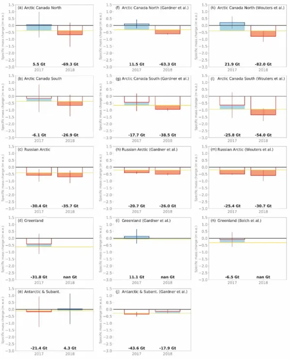
Figure S3 Ad hoc estimates of selected regional mass changes in 2016/17 and 2017/18 based on different reference datasets. The plots (a– e) in the left column correspond to plots in Fig. 1 using Zemp et al. (2019) as reference dataset but for the reference period 2003/04– 2008/09. The plots in the middle column (f–j) use Gardner et al. (2013, 2003/04–2008/09) as reference dataset. The plots in the right column (k–n) are using Wouters et al. (2019, 2005/06–2014/15) or Bolch et al. (2013, 2003/04–2007/08) as reference dataset. Note that

5

within a region, the annual anomalies (pale blue and pale red) are similar but absolute mass changes (in Gt) vary strongly in case of different mass-change rates in the reference datasets. For Greenland (d, i, n), no ad hoc estimate were calculated for 2017/18 because the glaciological observations are from a glacier without data in the reference periods.

7

Figure S4 Annual global mass changes in comparison between the ad hoc estimates of this study and the reference dataset by Zemp et al. (2019). The comparison is shown for the ad hoc estimates as based on the full glaciological sample of corresponding years (a) and for the WGMS reference glaciers only (b). The linear regression refers to the fit between the values (green) over the validation period

5

(2006/07−2015/16, cf. Fig. 2).