Design of a dual beam optical trap

Design of a Dual Beam Optical Trap

by

Tom Frejowski

Submitted to the Department of Mechanical Engineering

in partial fulfillment of the requirements for the degree of

Bachelor of Science in Mechanical Engineering

at the

MASSACHUSETTS INSTITUTE OF TECHNOLOGY

June 2019

© Massachusetts Institute of Technology 2019. All rights reserved.

Author . . . .

Department of Mechanical Engineering

May 17, 2019

Certified by . . . .

Ian W. Hunter

Hatsopoulos Professor of Mechanical Engineering

Thesis Supervisor

Accepted by . . . .

Maria Yang

Associate Professor of Mechanical Engineering

Undergraduate Officer

Design of a Dual Beam Optical Trap

by

Tom Frejowski

Submitted to the Department of Mechanical Engineering on May 17, 2019, in partial fulfillment of the

requirements for the degree of

Bachelor of Science in Mechanical Engineering

Abstract

Dual beam optical traps use radiation pressure from two counterpropagating laser beams to manipulate microscopic particles. Typical traps use optical fibers to guide those beams. This thesis proposes a design for the coaxial alignment of optical fibers that allows for the fibers to translate along a common axis while maintaining align-ment. Additionally, this design enables the optical fibers and trapping samples to be quickly and easily swapped out for different experiments. A full optical trapping setup was constructed using this design and successfully demonstrated the trapping of multiple polystyrene microspheres.

Thesis Supervisor: Ian W. Hunter

Acknowledgments

I would like to thank everyone at the BioInstrumentation Lab for their support over the course of this last semester. To Prof. Ian Hunter, for the opportunity to work on this project. To Dr. Ashin Modak and Dr. Cathy Hogan, for sharing their wisdom throughout this process. And to Dr. Micheal Zervas, for introducing me to the world of optics.

I owe a great deal to everyone who has taught me anything about design and fabrication, specifically Prof. Alexander Slocum, Dr. Daniel Braunstein, the Pap-palardo Lab shop staff: Bill Cormier, Jim Dudley, Steve Haberek, and Tasker Smith, the Hobby Shop staff: Hayami Arakawa and Coby Unger, and most importantly, my father, who practices craftsmanship in every aspect of his life and has taught me to do the same.

Contents

1 Background 6

1.1 Optical Trapping . . . 6

1.2 Dual Beam Optical Traps . . . 8

1.3 Optical Tweezers . . . 10

2 Design of the Dual Beam Fiber Optic Trap 13 2.1 System Level Architecture . . . 14

2.2 Laser Setup . . . 15

2.3 Alignment of Optical Fibers . . . 17

2.4 Imaging Setup . . . 22

3 Validation of the Optical Trap 25 3.1 Fiber Alignment . . . 25

3.2 Trapping 1 Micrometer Polystyrene Microspheres . . . 26

4 Conclusion and Future Steps 27

List of Figures

1-1 Scattering and Gradient Forces on a Particle in a Gaussian Beam . . 7

1-2 Beam Divergence from an Optical Fiber . . . 8

1-3 Graphic of Dual Beam Fiber Optic Trapping . . . 9

1-4 Forces on a Particle in Optical Tweezers . . . 11

1-5 Diagram of a Basic Optical Tweezer Setup . . . 12

2-1 Architectures for a Dual Beam Fiber Optic Trap . . . 14

2-2 Diagram of Dual Beam Fiber Optic Trap with Single Fiber Coupled Laser Source . . . 16

2-3 Technique for Aligning Optical Fibers Using Ceramic Ferrules and a V-groove . . . 18

2-4 Partially Exploded View of Differential Screw Assembly . . . 18

2-5 Cross Section View of Differential Screw Assembly . . . 19

2-6 Detail of Optical Fiber Retention Within the Differential Screw Assembly 20 2-7 Full Exploded View of the Differential Screw Assembly . . . 21

2-8 Fiber Alignment Assembly . . . 21

2-9 Imaging Setup . . . 22

2-10 Complete Dual Beam Fiber Optic Trapping Setup . . . 24

3-1 Microscope Image of Aligned Optical Fibers . . . 25 3-2 One Micrometer Polystyrene Beads Aligned in the Dual Beam Trap . 26

1 Background

1.1

Optical Trapping

Optical trapping is the use of radiation pressure from a laser beam to manipulate microscopic particles. Any discussion of optical trapping must acknowledge the work of Arthur Ashkin, who discovered the phenomenon in 1970 [1] and has since applied it to manipulate particles across a broad range of scales, from individual atoms [2] to biological cells [3, 5]. Optical trapping techniques have enabled breakthroughs in physics, chemistry, and biology and Ashkin’s contribution to all of these fields was recognized with the 2018 Nobel Prize in Physics.

Optical trapping relies on two distinct forces resulting from radiation pressure: scattering forces and gradient forces. A scattering force points in the direction of propagation of the beam and thus pushes particles along the beam axis. A particle that completely reflects any incident light straight back along the beam axis will only experience a net scattering force. In the case where light can refract through the particle, incident rays will exit the particle at some angle with respect to the beam axis and cause off-axis forces. If the incident beam does not have a spatially varying intensity profile or if the particle is oriented along the axis of a beam with a symmetric intensity profile, then the sum of all the off-axis forces will still result in only a net scattering force that pushes the particle along the beam axis. However, if the beam’s intensity profile is spatially varying and the particle does not lay on the beam axis, then the particle will experience a gradient force that pushes the particle perpendicular to the beam axis in addition to the scattering force [3]. This is because

the intensity of the rays refracting through the particle are not spatially constant, so their off-axis force contributions do not perfectly cancel. Figure 1-1 shows the force balance for a particle that lays along the axis of a beam with a 2D Gaussian intensity profile as well as an off-axis particle in the same beam.

Figure 1-1: (a) A particle with a higher refractive index than the surrounding media. The laser beam intensity profile is Gaussian as shown by the curve at the left. Since the particle sits on the axis of the beam, the force contributions of individual rays sum to a net scattering force that only points along the axis of the beam. (b) The same beam and particle, except the particle no longer sits on the beam axis. Ray 1 has a higher intensity than Ray 2 and produces a higher magnitude force on the particle. The sums of force contributions from the refracting rays result in a scattering force just as before, but now with the addition of a gradient force that is orthogonal to the scattering force and pushes the particle to the center of the beam.

For typical Gaussian laser beams, the gradient force will always point towards the beam axis, provided that the particle has a higher refractive index than the surround-ing media. This is particularly advantageous for manipulatsurround-ing particles because they will tend to be drawn in to the beam and self-center on its axis.

1.2

Dual Beam Optical Traps

While gradient forces are useful for positioning particles along the beam axis, scat-tering forces make capturing particles and keeping them still quite difficult because particles will accelerate along the beam axis. Ashkin immediately recognized this difficulty during his discovery in 1970 and proposed a method of trapping particles in three dimensions by using two mildly focused beams directed at each other [1]. If the beams are coaxial and have the same power, then a particle can be stably trapped between the two beams because the scattering forces from each beam are equal and opposite.

A dual beam optical trap can be created by aligning two free space laser beams1

and focusing each with a lens. However, a more common implementation of dual beam traps uses two coaxially aligned optical fibers to guide the beams towards each other. Optical fibers present several advantages over the free space laser approach, including simplified management and direction of the beams as well as eliminating the need for lenses, since a beam exiting a flat cleaved fiber will diverge at angle equal to the arcsine of the numerical aperture (NA) of the fiber as shown in Figure 1-2.

Figure 1-2: Beam divergence from an optical fiber. The divergence angle θ is related to the numerical aperture, NA of the fiber through θ = arcsin(NA).

Perhaps the most famous application of dual beam fiber optic traps is the work of Jochen Guck, who used the setup to measure the mechanical properties of biological cells [9, 8]. Guck found that at high laser powers, particles trapped in dual beam traps

will actually deform along the axis of the trap. By correlating the incident laser power with the forces on the cells and observing the deformation through a microscope, cell elasticity could be measured. Other variations of dual beam laser traps enable the controlled rotation of trapped particles by using asymmetric beams [11].

Figure 1-3: Graphic of dual beam fiber optic trapping.

Alignment of the two optical fibers is critical for the proper function of a dual beam fiber optic trap. Misaligned fibers can cause particles to oscillate between the beams or fail to be trapped altogether [6]. Another challenge with dual beam traps is introducing particles into the beam path. Various techniques used by researchers for dealing with these two obstacles are presented below.

One of the earliest demonstrations of a dual beam fiber optic trap, performed by Constable, et al. [6]. This demonstration featured a scheme for aligning the optical fibers by preloading them against a glass slide and a cylinder so that each fiber is tangent to the slide and cylinder. This forms two line contacts that constrain the X and Y translational motion as well as the pitch and yaw rotational motion of the fiber.2 _{The fibers are free to translate along the trap axis, which provides the}

advantage of variable spacing between the two fiber ends, which is helpful in tuning the strength and stability of the trap [6]. However, because this setup requires an uninterrupted cylinder to run behind both optical fibers, it is difficult to introduce a flow of particles that runs perpendicular to the trap axis. With this setup, researchers can only introduce samples into the trap by depositing a pool of fluid around the fiber

ends. Furthermore, these pools are unsealed and because of this are likely to evaporate away.

Glass capillaries present themselves as a good option for introducing samples into dual beam traps because they grant researchers the ability to flow samples in and out of the trap and can be sealed to prevent evaporation. However, typical hollow cylindrical glass capillaries cause lensing effects when light is passed through them, making it difficult to produce a trap as well as image the particles inside of the capillary. For these reasons, most fiber optic traps use hollow square capillary tubing to deliver samples into the beam path.

Setups that use square capillary tubing typically align the tubing and the optical fibers on a substrate with channel-like features for the capillary and fibers to rest in. The channel features are created by etching glass slides or epoxy-based photoresists and the entire assembly is often potted with PDMS, an optically clear silicon-based polymer, to keep all the components in place [18]. This technique makes for a robust and simple assembly, but the PDMS prohibits the adjustment of fiber separation and makes it difficult for researchers to reuse the fibers or swap out the capillary and thus limits some of the functionality offered by the alignment technique described by Constable, et al. [6]. Because of this, it is not apparent that a dual beam fiber optic trap exists that can accommodate a flow channel perpendicular to the trap axis and has easily adjustable fiber spacing.

1.3

Optical Tweezers

Dual beam optical traps were a natural extension of Ashkin’s 1970 findings, but it was over a decade before Ashkin successfully demonstrated the three dimensional trapping of particles using only a single laser beam [4]. These single beam traps were dubbed “Optical Tweezers” for the new level of dexterity that they brought to optical trapping. The creation of such a trap would require that a force act in the opposite direction of the propagation of the beam. This is achieved by passing the beam through a microscope objective with a high NA that sharply converges the

beam and the resulting forces on the particle point in the direction of the focal point of the beam [4]. Figure 1-4 shows the net force pushing a particle towards the focal point of the beam in scenarios where the particle is either in front of or behind the focal point.

Figure 1-4: Forces on a particle in an optical tweezer trap. The beam is focused through a high NA objective (simplified as a lens in this diagram). (a) A particle behind the focal point of the beam will experience a net force that pushes it forward towards the focus. (b) A particle in front of the focal point will experience a net force that pushes it backwards toward the focus.

Basic optical tweezer setups can be constructed using a few standard optical com-ponents. Figure 1-5 shows a diagram for a bare bones setup. A wide assortment of components can be added to basic tweezer setups to suit various imaging and trap-ping needs. Quadrant photodetectors can be added for high accuracy measurements of particle displacement [17]. A variety of filters can be placed in the imaging path to enhance imaging capabilities, like the use of crossed polarizing filters to capture the birefringence of trapped particles. Laser beam profiles can be transformed using special lenses, like axicons to create Bessel beams [14], or with spatial light modula-tors to create different trap geometries [7]. The use of optical trapping has ballooned since the 1980s and so has the number of variations on the basic trapping setup. To this day, researchers are still reapplying Ashkin’s fundamental findings from 1970.

2 Design of the Dual Beam Fiber

Optic Trap

This optical trap was initially developed as a tool for determining if optical trapping is a suitable technique for the manipulation and alignment of micro- and nano-scale building blocks to form larger structures. Several factors led to the choice of a dual beam trap over optical tweezers or other trapping setups for this particular applica-tion. Because of the high convergence of rays through the microscope objective, the trapping volumes of optical tweezers are limited to a small space around the focal point of the beam. This limitation can be circumvented through the use of holo-graphic optical tweezers, which create multiple traps from a single beam by using a spatial light modulator [7], however such setups are complex and require a fine con-trol of the beam to produce the desired results. The trapping volumes of dual beam traps are not as limited because particles are simply pushed between opposing beams rather than focused on a point. This makes dual beam traps a good candidate for aligning multiple particles about a single axis. Furthermore, optical tweezer setups have an imaging axis that is coupled to the trapping axis because they use the same microscope objective for both imaging and trapping the particles. A coupled imaging and trapping axis would make it difficult to visualize any particle alignment along the beam axis. Dual beam traps allow for the imaging axis to be orthogonal to the beam axis, making them favorable for this particular application.

2.1

System Level Architecture

As covered in Section 1.2, dual beam fiber optic traps are, in essence, just two optical fibers used to direct counterpropagating beams at each other. In practice, there are many ways to achieve this basic arrangement by varying the number of laser sources used and the methods for coupling the laser beams into the optical fibers.

Figure 2-1: Architectures considered for the design of the dual beam fiber optic trap.

Four distinct architectures were considered for this design and a schematic for each is shown in Figure 2-1. Two of the architectures feature free space lasers that are coupled into optical fibers by first collimating the beam exiting the laser source and

then capturing and introducing that beam into each fiber using a fiber coupler. One of the free space laser architectures uses two laser sources (one for each fiber), while the other splits a beam from one laser source using a beam splitting cube. Free space laser sources are common and available in a wide range of wavelengths and powers, but coupling these lasers into optical fibers requires elaborate setups and alignment procedures. The remaining two architectures are based on pigtailed laser sources, which come coupled to optical fibers directly from the manufacturer. Pigtailed laser sources circumvent the issues of coupling free space beams into fibers, but these sources are typically less common and more expensive than free space sources. As with the two free space laser architectures, the two pigtailed architectures feature one with two individual laser sources and one that has a single beam sources that passes through a fiber optic 50:50 Y-splitter which splits an incoming beam from one fiber into two fibers with equal power.

2.2

Laser Setup

Out of the four architectures presented in Section 2.1, the single pigtailed source split into fibers with a 50:50 Y-splitter was selected to simplify the setup and ensure that both beams operate at the same power, which is critical for maintaining a stable trap. Although this arrangement does not suffer from the power losses that are experienced when coupling a free space laser into an optical fiber, every fiber to fiber connection that the beam travels though will lose some power. The Y-splitter will also introduce some losses. For this architecture, the beam will travel through one fiber to fiber connection before being split and then each resulting beam will travel through another connection before exiting the optical fiber. The power lost at each fiber to fiber connection or splitting junction is called the insertion loss and is measured in [dB] and defined by manufacturers as:

Insertion Loss = 10 log Pin Pout

The optical fibers used in this setup are Corning HI980 single mode fibers termi-nated in an FC/APC connector. The fibers are connected to the Y-splitter using FC/APC mating sleeves (Thorlabs ADAFC4) which each have a specified insertion loss of <0.5 dB. The Y-splitter is a 50:50 split 980 nm narrowband splitter ( Thorlabs TN980R5A1B), which is specified to have a insertion loss of <3.9 dB for the beam path from the input to one of the outputs. The laser used (Qphotonics QFBGLD-980-500) outputs 980 nm wavelength light at a maximum power of 500 mW. The worst case total loss can be calculated step by step by tracing the path of the beam. That total loss is found to be 176 mW. With these losses, it is expected that the output power of each beam exiting the flat cleaved fiber is at least 162 mW. Considering that previous studies have demonstrated optical trapping in dual beam fiber optic traps at powers as low as 7 mW per fiber [6], this setup should provide sufficient power.

2.3

Alignment of Optical Fibers

Coaxial fiber alignment is critical to the performance of the dual beam trap. Princi-ples of precision design as well as tight tolerance components were used to ensure good fiber alignment in this setup. Most dual beam fiber optic traps use photolithography to create alignment features on a substrate, which requires specialized equipment and the resulting assembly must be potted to maintain the positions of components. For experimental setups that require the spacing between optical fibers to be adjusted or for setups that must be disassembled and reassembled, the photolithography tech-nique is not particularly optimal. A setup that can be fully disassembled and re-assembled is favorable for many reasons; the capillaries that contain the samples can easily be switched out if they become dirty or a different sample needs to be used and the optical fibers can be replaced if they fracture or if an experiment requires fibers that operate on a different wavelength band.

To achieve a design that was fully rebuildable, allowed for adjustment of the fiber-to-fiber spacing, and provided good coaxial alignment of the optical fibers, the bare fiber ends were threaded through commercially available ceramic ferrules (Thorlabs CFLC126-10). These ferrules are typically used for terminating fibers and so are designed with tight tolerances (+3/-0µm on the inner bore diameter and +0.5/-1 µm on the outer diameter of the ferrule) [16]. These ferrules are then aligned coaxially with respect to each other using a V-groove that was machined into an aluminum plate with a 3 mm diameter 90◦ end mill. A cylinder resting in a V-groove will have two line contacts that together constrain four of its degrees of freedom (X/Y translation and pitch/yaw rotation when Z is the axis of the cylinder). The two other unconstrained degrees of freedom (Z translation and roll rotation) are not critical for coaxial alignment.

Because the bare fiber ends are threaded through the ferrules, the fibers are free to translate on the axis that they are aligned along. This enables the spacing between the ends of the fibers to be adjusted without disturbing their alignment. In addition to this, it is important to have a method for translating the fibers in a controlled manner

Figure 2-3: Proposed technique for aligning optical fibers using ceramic ferrules and a V-groove.

so that the fiber-to-fiber spacing can be precisely adjusted. To achieve this functional requirement, a differential screw positioning system was designed and fabricated. Figure 2-4 shows a partially exploded view of the differential screw assembly, which is composed of the head screw, an outer sleeve, a thumb screw, and a wave spring to preload the assembly and minimize backlash.

Figure 2-4: Partially exploded view of the differential screw assembly.

Differential screws provide much finer movement than traditional screws by ex-ploiting a small difference in the thread pitch between two screws. The “virtual pitch”

of a differential screw is described by:

Pvirtual = P1− P2, (2.2)

where Pvirtual is the virtual pitch of the entire differential screw system, P1 is the

larger pitch in the assembly and P2 is the smaller pitch. The two screw threads

used in this setup were M6-0.75 and M4-0.7. When configured together, these give a virtual pitch of 0.05 mm, which means that for every full rotation of the thumb screw input, the differential screw head moves 0.05 mm (50 µm).

Figure 2-5: Cross section view of differential screw assembly. The head screw subassembly is shown in green and the thumb screw is shown in blue.

The thumb screw features M6-0.75 external threads to mate to the outer sleeve and M4-0.7 internal threads to mate to the head screw. The head screw features a keyway so it does not rotate with respect to the outer sleeve. As the thumb screw is screwed into the outer sleeve, the screw head is pulled into the internal bore of the the thumb screw. For each rotation of the thumb screw, the thumb screw moves 0.75 mm with respect to the outer sleeve, while the head screw moves 0.7 mm in the opposite direction with respect to the thumb screw. This results in a net movement of 0.05 mm of the head screw with respect to the outer sleeve for every full rotation of the thumb screw.

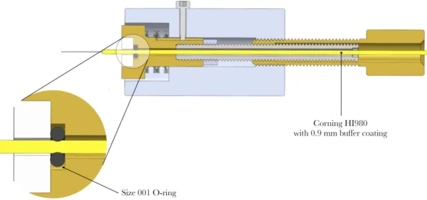
fiber, each component in the differential screw assembly was bored hollow so that the fiber could pass through. The optical fiber is retained by the head screw through a size 001 O-ring (0.74 mm ID, 2.77 mm OD) that grips the 0.9 mm outer coating of the fiber. Because the head screw does not rotate with respect to the outer sleeve, the differential screw assembly does not produce any torsional stress on the optical fiber.

The overall range of motion of each differential screw assembly is 1.5 mm. Coarse adjustments of the optical fiber’s position can be made by just sliding the fiber through the assembly, since the O-ring provides enough gripping pressure to retain the fiber, but not enough to permanently lock it in place.

Figure 2-6: Detail of optical fiber retention within the differential screw assembly. The entire differential screw assembly is hollow allowing for the optical fiber to pass through. A size 001 O-ring grips the fiber and couples the motion of the head screw to the optical fiber.

The head screw subassembly is composed of several pieces to simplify fabrication. The M4-0.7 screw thread is composed of a modified vented screw, which came bored out already and eliminated the need to drill out a large aspect ratio hole. That modified screw is then secured to the internal threads in the screw shoulder with a lock nut so that it does not back out. In addition to being hollow, the screw shoulder has a stepped bore for the O-ring and a plastic plug that axially retains the O-ring. The screw shoulder’s smaller OD is machined for a slip fit within the bore of the outer

sleeve and rotation is prevented with a keyway that engages with an M1.6-0.35 screw threaded into the the outer sleeve.

Figure 2-7: a) Full exploded view of the differential screw assembly in CAD. b) All nine components after fabrication.

The entire fiber alignment assembly, consisting of two differential screw assemblies mounted to the V-groove sample stage, with two ferrules and preload O-rings is shown in Figure 2-8.

Figure 2-8: Complete fiber alignment assembly. The right panel shows the fiber alignment assembly mounted to the XYZ stage of the imaging setup.

Samples for optical trapping are contained in a square capillary (VitroCom 8510) with a 100 µm inner width and a 200 µm outer width. Square capillaries must be

used rather than the more common round capillaries in order to avoid distorting the laser beams and the image through curved surfaces.

2.4

Imaging Setup

To image any particles that are captured in the dual beam trap, a simple upright optical microscopy setup is used. It consists of an LED light source that is collimated through a plano-convex lens (F = 25.4 mm, Thorlabs LA1252-A), a 60× 0.8 NA infinity corrected microscope objective (Nikon CFI Achromat series) and a bi-convex lens (F = 100 mm, Thorlabs LB1676) which images onto a 1280×1024 pixel CMOS sensor (Thorlabs DCC1645C).

Figure 2-9: Optical microscopy setup used for imaging trapped particles.

Criterion,

r = 1.22λ

NA , (2.3)

where r represents the minimum resolvable distance between features, λ is the working wavelength (assuming a minimum of 400 nm for this setup), and NA is the numerical aperture of the objective (0.8 in this case). This gives a minimum resolvable distance of 610 nm between features for this setup.

The fiber alignment assembly rests on a stage which can move in XYZ relative to the imaging setup. X/Y adjustments are made through a slip plate, while Z adjustments (focus) are made with a Newport M-MVN120 vertical stage.

3 Validation of the Optical Trap

3.1

Fiber Alignment

To verify that the ferrules and V-groove are indeed aligning the optical fibers, the bare fibers were inserted into the alignment assembly and imaged without a capillary in between them. Figure 3-1 shows the two fibers under a 20× and 60× objective.

Figure 3-1: (a) Optical fibers inserted into alignment assembly at 20× magnification. (b) Optical fibers inserted into alignment assembly at 60× magnification.

The transverse distance between the cores of the optical fibers was measured off of these microscope images with ImageJ and found to be 2 ± 0.5 µm. The angular mismatch was measured to be 0.025 ± 0.013◦.

3.2

Trapping 1 Micrometer Polystyrene Microspheres

To confirm the function of the entire optical trapping setup, the sample capillary was loaded with an aqueous solution of 1µm polystyrene microspheres (Polysciences, Inc cat#24287). Laser power was monitored indirectly by monitoring the current from the current controller and correlating that to the laser’s current-power curve provided by the manufacturer. Laser power was slowly increased until trapping of the beads was achieved at a power of approximately 230 mW. Factoring in all the losses described in Section 2.2, the output power per fiber was about 74 mW when trapping first occurred. Figure 3-2 shows stills from a video taken during a trapping test. Note that several beads can be aligned along the axis of the trap.

Figure 3-2: (a) Image of 1µm polystyrene beads in the sample capillary, with the laser turned off. (b) Alignment of polystyrene beads along the trapping axis while the laser is turned on. Both images are captured from a video taken under 60× magnification.

In Figure 3-2 you may notice some refraction of the laser beams, which is particu-larly pronounced at the vertical walls of the square capillary, right where the optical fibers are butted against the capillary. To minimize this refraction, an index matching gel could be applied at the interface between the capillary face and the flat cleaved fiber end [12].

4 Conclusion and Future Steps

The successful assembly and operation of the dual beam optical trap presented in this paper shows that a fiber optical trap can be constructed with basic mechanical components and without the need for the specialized photolithography equipment typically used to fabricate dual beam traps. Furthermore, the presented design offers several advantages over the typical methods for creating optical fiber based dual beam traps: the separation between fiber ends can be adjusted to sub-micron resolution using the differential screw assembly, the capillary tubing for containing samples can be easily swapped out without having to make a new assembly, and the optical fibers can be replaced if they break or need to be replaced for any other reason. It is my hope that this new design will enable researchers working with dual beam optical fiber traps to have greater control over their setup and perform experiments quickly with less headaches.

While trapping polystyrene microspheres is a great way to demonstrate the func-tion of the optical trap, this does not represent the full extent of a dual beam trap’s capabilities. As demonstrated by Guck, et al. these traps can be used to capture and stretch biological cells to examine their mechanical properties [8]. Modified dual beam traps can also be used to rotate trapped particles in order to perform cell tomography [11].

One particularly exciting application of optical trapping is the assembly of micro-and nano-scale structures by individually manipulating particles. Pauzauskie, et al. has demonstrated the use of optical tweezers to create assemblies from semiconductor nanowires [15]. Similar techniques could be used to create material structures in dual beam traps. As demonstrated with the polystyrene microspheres, dual beam optical

traps lend themselves well to aligning multiple particles along a single axis. This fact can be leveraged for assembling macro-scale materials out of nano-scale components where the alignment of the components is important to the material properties. Cel-lulose nanofibrils are an example of such a material. Individual celCel-lulose nanofibrils are approximately 5 nm in diameter and on the order of hundreds of nanometers long [10]. Individual nanofibrils have been shown to have a modulus of elasticity between 130 to 150 GPa and yield strengths as high as 3 GPa, which rival the properties of many high strength steels [13]. However, translating these properties to macro-scale materials is difficult because the macro-macro-scale strength and modulus is highly dependent on the alignment of individual fibrils within the structure. Dual beam traps could be used to axially align cellulose nanofibrils to create larger bundles of nanofibrils that could possibly preserve the mechanical properties of individual fibrils. The optical trapping setup presented in this paper could be augmented to test this proposal. Currently, the limiting factor of the setup is the resolution of the imagining system, which would be unable to resolve individual cellulose nanofibrils to confirm their alignment along the trap axis. Thus the imaging setup would need to be converted to one of higher resolution, perhaps using confocal microscopy or tagging the the nanofibrils with flourophores and using super-resolution fluorescence microscopy.

Bibliography

[1] A. Ashkin. Acceleration and trapping of particles by radiation pressure. Physical review letters, 24(4):156, 1970.

[2] A. Ashkin. Trapping of atoms by resonance radiation pressure. Phys. Rev. Lett., 40:729–732, Mar 1978.

[3] A. Ashkin. History of optical trapping and manipulation of small-neutral particle, atoms, and molecules. IEEE Journal of Selected Topics in Quantum Electronics, 6(6):841–856, 2000.

[4] A. Ashkin, J. M. Dziedzic, J. Bjorkholm, and S. Chu. Observation of a single-beam gradient force optical trap for dielectric particles. Optics letters, 11(5):288– 290, 1986.

[5] A. Ashkin, J. M. Dziedzic, and T. Yamane. Optical trapping and manipulation of single cells using infrared laser beams. Nature, 330(6150):769, 1987.

[6] A. Constable, J. Kim, J. Mervis, F. Zarinetchi, and M. Prentiss. Demonstration of a fiber-optical light-force trap. Optics letters, 18(21):1867–1869, 1993.

[7] J. E. Curtis, B. A. Koss, and D. G. Grier. Dynamic holographic optical tweezers. Optics communications, 207(1-6):169–175, 2002.

[8] J. Guck, R. Ananthakrishnan, H. Mahmood, T. J. Moon, C. C. Cunningham, and J. K¨as. The optical stretcher: a novel laser tool to micromanipulate cells. Biophysical journal, 81(2):767–784, 2001.

[9] J. Guck, R. Ananthakrishnan, T. J. Moon, C. C. Cunningham, and J. K¨as. Optical deformability of soft biological dielectrics. Phys. Rev. Lett., 84:5451– 5454, Jun 2000.

[10] A. Isogai. Cellulose nanofibers as new bio-based nanomaterials. In High-Performance and Specialty Fibers, pages 297–311. Springer, 2016.

[11] Moritz K Kreysing, T. Kießling, A. Fritsch, C. Dietrich, J. Guck, and J. A. K¨as. The optical cell rotator. Optics Express, 16(21):16984–16992, 2008.

[12] B. Lincoln, S. Schinkinger, K. Travis, F. Wottawah, S. Ebert, F. Sauer, and J. Guck. Reconfigurable microfluidic integration of a dual-beam laser trap with biomedical applications. Biomedical microdevices, 9(5):703–710, 2007.

[13] N. Mittal, F. Ansari, Krishne Gowda. V, C. Brouzet, P. Chen, P. T. Larsson, S. V. Roth, F. Lundell, Lars Wagberg, N. A. Kotov, et al. Multiscale control of nanocellulose assembly: Transferring remarkable nanoscale fibril mechanics to macroscale fibers. ACS nano, 12(7):6378–6388, 2018.

[14] T. Paprotta, B. Esembeson, L. Eichner, J. Schumacher, S. C. Wasserman, and A. E. Cable. The bessel-beam random access trap. In Complex Light and Opti-cal Forces VI, volume 8274, page 82740O. International Society for Optics and Photonics, 2012.

[15] P. J. Pauzauskie, A. Radenovic, E. Trepagnier, H. Shroff, P. Yang, and J. Liphardt. Optical trapping and integration of semiconductor nanowire as-semblies in water. Nature materials, 5(2):97, 2006.

[16] A. H. Slocum. Precision machine design. Society of Manufacturing Engineers, 1992.

[17] K. Visscher, S. P Gross, and S. M. Block. Construction of multiple-beam opti-cal traps with nanometer-resolution position sensing. IEEE Journal of Selected Topics in Quantum Electronics, 2(4):1066–1076, 1996.

[18] T. Yang, F. Bragheri, and P. Minzioni. A comprehensive review of optical stretcher for cell mechanical characterization at single-cell level. Micromachines, 7(5):90, May 2016.