HAL Id: hal-03048687
https://hal.umontpellier.fr/hal-03048687
Submitted on 9 Dec 2020
HAL is a multi-disciplinary open access
archive for the deposit and dissemination of
sci-entific research documents, whether they are
pub-lished or not. The documents may come from
teaching and research institutions in France or
abroad, or from public or private research centers.
L’archive ouverte pluridisciplinaire HAL, est
destinée au dépôt et à la diffusion de documents
scientifiques de niveau recherche, publiés ou non,
émanant des établissements d’enseignement et de
recherche français ou étrangers, des laboratoires
publics ou privés.
B. Hoogakker, R. Smith, J. Singarayer, R. Marchant, I. Prentice, J. Allen, R.
Anderson, S. Bhagwat, H. Behling, O. Borisova, et al.
To cite this version:
B. Hoogakker, R. Smith, J. Singarayer, R. Marchant, I. Prentice, et al.. Terrestrial biosphere changes
over the last 120 kyr. Climate of the Past, European Geosciences Union (EGU), 2016, 12 (1), pp.51-73.
�10.5194/cp-12-51-2016�. �hal-03048687�
www.clim-past.net/12/51/2016/ doi:10.5194/cp-12-51-2016
© Author(s) 2016. CC Attribution 3.0 License.
Terrestrial biosphere changes over the last 120 kyr
B. A. A. Hoogakker1, R. S. Smith2, J. S. Singarayer3,4, R. Marchant5, I. C. Prentice6,7, J. R. M. Allen8,
R. S. Anderson9, S. A. Bhagwat10, H. Behling11, O. Borisova12, M. Bush13, A. Correa-Metrio14, A. de Vernal15,
J. M. Finch16, B. Fréchette15, S. Lozano-Garcia14, W. D. Gosling17, W. Granoszewski18, E. C. Grimm19, E. Grüger11,
J. Hanselman20, S. P. Harrison7,21, T. R. Hill16, B. Huntley8, G. Jiménez-Moreno22, P. Kershaw23, M.-P. Ledru24,
D. Magri25, M. McKenzie26, U. Müller27,28, T. Nakagawa29, E. Novenko12, D. Penny30, L. Sadori25, L. Scott31,
J. Stevenson32, P. J. Valdes4, M. Vandergoes33, A. Velichko12, C. Whitlock34, and C. Tzedakis35
1Department of Earth Science, University of Oxford, South Parks Road, Oxford, OX1 3AN, UK 2NCAS-Climate and Department of Meteorology, University of Reading, Reading, UK
3Department of Meteorology and Centre for Past Climate Change, University of Reading, Reading, UK 4BRIDGE, School of Geographical Sciences, University of Bristol, University Road, Bristol, BS8 1SS, UK 5Environment Department, University of York, Heslington, York, YO10 5DD, UK
6AXA Chair of Biosphere and Climate Impacts, Grand Challenges in Ecosystems and the Environment and Grantham
Institute – Climate Change and the Environment, Imperial College London, Department of Life Sciences, Silwood Park Campus, Buckhurst Road, Ascot, SL5 7PY, UK
7Department of Biological Sciences, Macquarie University, North Ryde, NSW 2109, Australia 8Durham University, School of Biological and Biomedical Sciences, Durham, DH1 3LE, UK
9School of Earth Sciences and Environmental Sustainability, Box 5964 Northern Arizona University, Flagstaff, Arizona
86011, USA
10The Open University, Walton Hall, Milton Keynes, MK7 6AA, UK
11Department of Palynology and Climate Dynamics, Albrecht von Haller Institute for Plant Sciences, University of
Göttingen, Untere Karspüle 2, 37073 Göttingen, Germany
12Institute of Geography, Russian Academy of Sciences, Staromonetny Lane 19, 119017 Moscow, Russia 13Florida Institute of Technology, Biological Sciences, Melbourne, FL 32901, USA
14Instituto de Geología, Universidad Nacional Autónoma de México, Cd. Universitaria, 04510, DF, Coyoacan, Mexico 15GEOTOP, Université du Québec à Montréal, C.P. 8888, Succursale Centre-Ville, Montréal, QC, H3C 3P8, Canada 16School of Agricultural, Earth and Environmental Science, University of KwaZulu-Natal, Private Bag X01, Scottsville,
3209, South Africa
17Palaeoecology & Landscape Ecology, IBED, Faculty of Science, University of Amsterdam, P.O. Box 94248, 1090 GE
Amsterdam, the Netherlands
18Polish Geological Institute – National Research Institute, Carpathian Branch, Skrzatów 1, 31-560 Kraków, Poland 19Illinois State Museum, Research and Collections Center, 1011 East Ash Street, Springfield, IL 62703, USA 20Westfield State University, Department of Biology, Westfield, MA 01086, USA
21Centre for Past Climate Change and School of Archaeology, Geography and Environmental Sciences (SAGES), University
of Reading, Whiteknights, RG6 6AH, Reading, UK
22Departamento de Estratigrafía y Paleontología, Facultad de Ciencias, Universidad de Granada, Avda. Fuente Nueva S/N,
18002 Granada, Spain
23School of Geography and Environmental Science, Monash University, Melbourne, VIC 3800, Australia
24IRD UMR 226 Institut des Sciences de l’Evolution - Montpellier (ISEM) (UM2 CNRS IRD) Place Eugène Bataillon cc
061, 34095 Montpellier CEDEX, France
25Sapienza University of Rome, Department of Environmental Biology, 00185 Rome, Italy
26Monash University, School of Geography and Environmental Science, Clayton, VIC 3168, Australia 27Biodiversity and Climate Research Centre (BiK-F), 60325 Frankfurt, Germany
28Institute of Geosciences, Goethe University Frankfurt, 60438 Frankfurt, Germany 29Ritsumeikan University, Research Centre for Palaeoclimatology, Shiga 525-8577, Japan
30School of Geosciences, The University of Sydney, NSW 2006, Australia
31University of the Free State, Faculty of Natural and Agricultural Sciences, Plant Sciences, Bloemfontein 9300, South Africa 32Department of Archaeology and Natural History, ANU College of Asia and the Pacific, Australian National University,
Canberra, ACT 0200, Australia
33University of Maine, Climate Change Institute, Orono, ME 04469-5790, USA
34Montana State University, Department of Earth Sciences, Bozeman, MT 59717-3480, USA 35UCL Department of Geography, Gower Street, London, WC1E 6BT, UK
Correspondence to: B. A. A. Hoogakker ([email protected])
Received: 23 January 2015 – Published in Clim. Past Discuss.: 31 March 2015
Revised: 30 November 2015 – Accepted: 14 December 2015 – Published: 18 January 2016
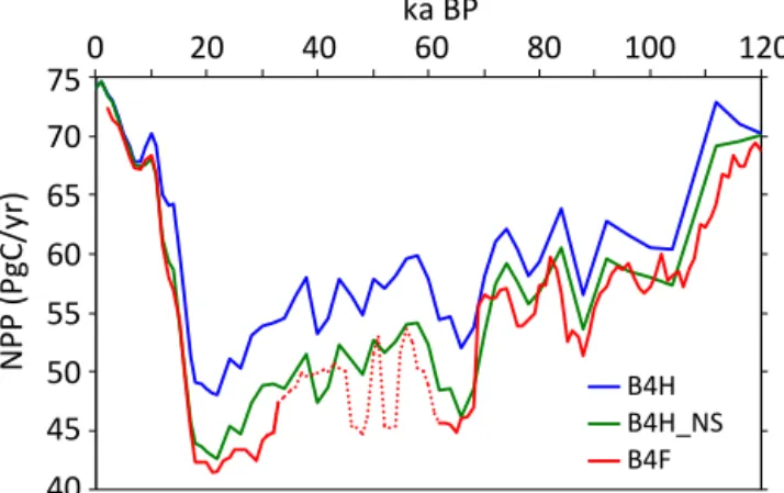
Abstract.A new global synthesis and biomization of long (> 40 kyr) pollen-data records is presented and used with sim-ulations from the HadCM3 and FAMOUS climate models and the BIOME4 vegetation model to analyse the dynamics of the global terrestrial biosphere and carbon storage over the last glacial–interglacial cycle. Simulated biome distribu-tions using BIOME4 driven by HadCM3 and FAMOUS at the global scale over time generally agree well with those in-ferred from pollen data. Global average areas of grassland and dry shrubland, desert, and tundra biomes show large-scale increases during the Last Glacial Maximum, between ca. 64 and 74 ka BP and cool substages of Marine Isotope Stage 5, at the expense of the tropical forest, warm-temperate forest, and temperate forest biomes. These changes are re-flected in BIOME4 simulations of global net primary pro-ductivity, showing good agreement between the two models. Such changes are likely to affect terrestrial carbon storage, which in turn influences the stable carbon isotopic composi-tion of seawater as terrestrial carbon is depleted in13C.
1 Introduction
Variations in global climate on multi-millennial timescales have caused substantial changes to terrestrial vegetation dis-tribution, productivity, and carbon storage. Periodic varia-tions in the Earth’s orbital configuration (axial tilt with a ∼41 kyr period, precession with ∼ 19 and 23 kyr periods, and eccentricity with ∼ 100 kyr and longer periods) result in small variations in the seasonal and latitudinal distribution of insolation, amplified by feedback mechanisms (Berger, 1978). For the last ∼ 0.8 million years, long glacial peri-ods have been punctuated by short interglacials on roughly a 100 kyr cycle. Glacial periods are associated with low at-mospheric CO2concentrations, lowered sea level, and
exten-sive continental ice sheets; interglacial periods are associated with high (similar to pre-industrial) CO2concentrations, high
sea level, and reduced ice sheets (Petit et al., 1999; Peltier et al., 2004; Lüthi et al., 2008).
During glacial–interglacial cycles the productivity and car-bon storage of the terrestrial biosphere are influenced by or-bitally forced climatic changes and atmospheric CO2
con-centrations. Expansion of ice sheets during glacial periods caused a significant loss of land area available for coloniza-tion, but this was largely compensated for by the exposure of continental shelves due to lower sea level. The terrestrial biosphere (vegetation and soil) is estimated to contain around 2000 PgC (Prentice et al., 2001) plus a similar quantity stored in peatlands and permafrost (Ciais et al., 2012). During the last glacial period the terrestrial biosphere was significantly reduced. It has been estimated that the terrestrial biosphere contained 300 to 700 PgC less carbon during the Last Glacial Maximum (LGM, 21 ka BP) compared with pre-industrial times (Bird et al., 1994; Ciais et al., 2012; Crowley et al., 1995; Duplessy et al., 1988; Gosling and Holden, 2011; Köh-ler and Fischer, 2004; Prentice et al., 2011). As first noted by Shackleton et al. (1977), the oceanic inventory of carbon isotopes (δ13C) is influenced by terrestrial carbon storage be-cause terrestrial organic carbon has a negative signature, due to isotopic discrimination during photosynthesis. Many of the estimates of the reduction in terrestrial carbon storage at the LGM have therefore been based on the observed LGM lowering of deep-ocean δ13C. A reduction in the terrestrial biosphere of this size would have contributed a large amount of CO2 to the atmosphere, although ocean carbonate
com-pensation would have reduced the expected CO2increase to
15 ppm over about 5 to 10 kyr (Sigman and Boyle, 2000). Many palaeoclimate data and modelling studies have fo-cused on the contrasts between the LGM, the mid-Holocene (6 ka BP), and the pre-industrial period. The BIOME 6000 project (http://www.bridge.bris.ac.uk/resources/Databases/ BIOMES_data) synthesized palaeovegetation records from many sites to provide global data sets for the LGM and mid-Holocene. Data syntheses are valuable in allowing re-searchers to see the global picture from scattered, individual records, and to enable model–data comparisons. The data can be interpreted in the context of a global, physically based model that allows the point-wise data to be seen in a coherent way. There are continuous, multi-millennial
Figure 1.Locations and altitudes of pollen records superimposed on pre-industrial HadCM3 orography (m).
pollen records that stretch much further back in time than the LGM but they have not previously been brought together in a global synthesis to study changes of the last glacial– interglacial cycle. These records can provide a global picture of transient change in the biosphere and the climate system. Here we have synthesized and biomized (Prentice et al., 1996) a number of these records (for locations see Fig. 1), providing a new data set of land biosphere change that covers the last glacial–interglacial cycle. In Sect. 2.1 we outline the biomization procedures applied to reconstruct land biosphere changes.
To improve understanding of land biosphere interac-tions with the ocean–atmospheric reservoir, we have mod-elled the terrestrial biosphere for the last 120 kyr, from the previous (Eemian) interglacial to the pre-industrial pe-riod. Details of the atmosphere–ocean general circulation model (AOGCM) climate and vegetation model simula-tions are provided in Sect. 2.2. In Sect. 3 we evaluate biome reconstructions based on our model outputs using the BIOME 6000 project (www.bridge.bris.ac.uk/resources/ Databases/BIOMES_data), and our new biomized synthe-sis of terrestrial pollen-data records, focusing on the pre-industrial period and 6 (mid-Holocene), 21 (LGM), 54 (a relatively warm interval in the last glacial period), 64 (a relatively cool interval in the glacial period), 84 (the early part of the glacial cycle), and 120 ka BP (the Eemian inter-glacial). The effects of rapid millennial-scale climate fluctua-tions were not simulated. Finally, in Sect. 4 we use our biome simulations to estimate net primary productivity.
2 Methods 2.1 Biomization
Biomization assigns pollen taxa to one or more plant func-tional types (PFTs). The PFTs are assigned to their respec-tive biomes and affinity scores are calculated for each biome
(sum of the square roots of pollen percentages contributed by the PFTs in each biome). This method was first devel-oped for Europe (Prentice et al., 1996) and versions of it have been applied to most regions of the world (Jolly et al., 1998; Takahara et al., 1999; Tarasov et al., 2000; Thomp-son and AnderThomp-son, 2000; Williams et al., 2000; Elenga et al., 2004; Pickett et al., 2004; Marchant et al., 2009). We ap-ply these regional PFT schemes (Table 1) to pollen records that generally extend > 40 kyr, assigning the pollen data to megabiomes (tropical forest, warm-temperate forest, tem-perate forest, boreal forest, savanna/dry woodland, grass-land/dry shrubland, desert, and tundra) as defined by Harri-son and Prentice (2003) in order to harmonize regional vari-ations in PFT to biome assignments and to allow globally consistent model–data comparisons.
Table 2 lists the pollen records used. Biomization matrices and megabiome score data can be found in the Supplement. For taxa with no PFT listing, the family PFT was used if part of the regional biomization scheme. Plant taxonomy was checked using itis.gov, tropicos.org, and the African Pollen Database. Pollen taxa can be assigned to more than one PFT either because they include several species in the genus or family, with different ecologies, or because they comprise species that can adopt different habitats in different environ-ments.
Age models provided with the individual records were used. However, in cases where radiocarbon ages were only provided for specific depths (e.g. Mfabeni, CUX), linear in-terpolations between dates were used to estimate ages for the remaining depths. Some age models may be less certain, especially at sites which experience variable sedimentation rates and/or erosion. Sometimes more than one age model accompanies the data, illustrating the range of ages and also that there can be large uncertainties. To aid comparison, for several southern European sites (e.g. Italy and Greece) it has been assumed that vegetation changes occurred syn-chronously within the age uncertainties of their respective chronologies, for which there is evidence (e.g. Tzedakis et al., 2004a).
2.2 Model simulations
Global simulations of vegetation changes over the last glacial cycle were produced using a vegetation model (BIOME4) forced offline using previously published climate simulations from two AOGCMs (HadCM3 and FAMOUS). By using two models we test the robustness of the reconstructions to differ-ent climate forcings.
2.2.1 HadCM3
HadCM3 is a general circulation model, consisting of cou-pled atmospheric model, ocean, and sea ice models (Gordon et al., 2000; Pope et al., 2000). The resolution of the atmo-spheric model is 2.5◦in latitude by 3.75◦in longitude by 19
Table 1.Details of the various biomization schemes applied for the different regions.
Africa Jolly et al. (1998)
Southeast Asia, Australia Pickett et al. (2004)
Japan Takahara et al. (1999)
Southern Europe Elenga et al. (2004) Northeastern Europe Tarasov et al. (2000)
North America: western north Thompson and Anderson (2000) North America: east and northeast Williams et al. (2000)
Latin America Marchant et al. (2009)
unequally spaced levels in the vertical. The resolution of the ocean is 1.25 by 1.25◦with 20 unequally spaced layers in the
ocean extending to a depth of 5200 m. The model contains a range of parameterizations, including a detailed radiation scheme that can represent the effects of minor trace gases (Edwards and Slingo, 1996). The land surface scheme used is the Met Office Surface Exchange Scheme 1 (MOSES1; Cox et al., 1999). In this version of the model, interactive vegetation is not included. The ocean model uses the Gent– McWilliams mixing scheme (Gent and McWilliams, 1990), and sea ice is a thermodynamic scheme with parameteriza-tion of ice drift and leads (Cattle and Crossley, 1995).
Multiple “snapshot” simulations covering the last 120 kyr have been performed with HadCM3. The boundary con-ditions and setup of the original set of simulations have been previously documented in detail in Singarayer and Valdes (2010). The snapshots were done at intervals of every 1 ka between the pre-industrial (PI) and LGM (21 ka BP), every 2 ka between the LGM and 80 ka BP, and every 4 ka between 80 and 120 ka BP. Boundary conditions are variable between snapshots but constant for each simulation. Orbital parameters are taken from Berger and Loutre (1991). Atmo-spheric concentrations of CO2were taken from a stacked ice
core record of Vostok (Petit et al., 1999) prior to 62 kyr, in-corporating Taylor Dome (Indermühle et al., 2000) to 22 kyr and EDC96 (Monnin et al., 2001) up to 0 kyr. CH4and N2O
were taken from EPICA (Spahni et al., 2005; Loulergue et al., 2008), and all greenhouse gas concentrations were on the EDC3 timescale (Parrenin et al., 2007). The prescription of ice sheets was achieved with ICE-5G (Peltier, 2004) for 0–21 ka BP, and extrapolated to the pre-LGM period from the ICE-5G reconstruction using the method described in Eriksson et al. (2012). The simulations were each spun up from the end of previous runs described in Singarayer and Valdes (2010) to adjust to the modified ice-sheet bound-ary conditions for 470 years. The monthly climatologies de-scribed hereafter are of model years 470–499. The model performs reasonably well in terms of glacial–interglacial global temperature anomaly (HadCM3 is in the middle of the distribution of global climate models and palaeoclimate reconstructions) and high-latitude temperature trends (al-though as with all models, the magnitude of the tempera-ture anomalies in the glacial is underestimated), as well as
at lower latitudes (Singarayer and Valdes, 2010; Singarayer and Burrough, 2015).
2.2.2 FAMOUS
FAMOUS (Smith, 2012) is an Earth System model, derived from HadCM3. It is run at approximately half the spatial res-olution of HadCM3 to reduce the computational expense as-sociated with AOGCM simulations without fundamentally sacrificing the range of climate system feedbacks of which it is capable. Pre-industrial control simulations of FAMOUS have both an equilibrium climate and global climate sensitiv-ity similar to that of HadCM3. A suite of transient FAMOUS simulations of the last glacial cycle, conducted with speci-fied atmospheric CO2, ice sheets, and changes in solar
inso-lation resulting from variation in the Earth’s orbit, compare well with the NGRIP, EPICA, and MARGO proxy recon-structions of glacial surface temperatures (Smith and Gre-gory, 2012). For the present study, we use the most realis-tically forced simulation of the Smith and Gregory (2012) suite (experiment ALL-ZH), forced with Northern Hemi-sphere ice sheets taken from the physical ice-sheet modelling work of Zweck and Huybrechts (2005), atmospheric CO2,
CH4, and N2O concentrations from the EPICA project (Lüthi
et al., 2008 and Spahni et al., 2005, mapped onto the EDC3 Parrenin et al., 2007, age scale) and orbital forcing from Berger (1978). The composite CO2record contained in Lüthi
et al. (2008) uses data from the Vostok core (Petit et al., 1999) between 22 and 393 kyr. The Vostok record is now believed (Bereiter et al., 2012) to be erroneously low during the early part of Marine Isotope Stage 3. For this reason, the FAMOUS results during this period are likely biased too cold. Although of a lower spatial resolution than HadCM3, these FAMOUS simulations have the benefit of being transient and represent-ing low-frequency variability within the climate system, as well as using more physically plausible ice-sheet extents be-fore the LGM than were used in the HadCM3 simulations. To allow the transient experiments to be conducted in a tractable amount of time, these forcings were all “accelerated” by a factor of 10, so that the 120 kyr of climate are simulated in 12model kyr – this method has been shown to have little ef-fect on the surface climate (Timm and Timmerman, 2007; Ganopolski et al., 2010), although it does distort the response
of the deep ocean. In addition, we did not include changes in sea level, Antarctic ice volume, or meltwater from ice sheets to enable the smooth operation of the transient simulations. The impact of ignoring the continental shelves exposed by lower sea levels will be discussed later; the latter two approx-imations are unlikely to have an impact over the timescales considered here. Although within the published capabilities of the model, interactive vegetation was not used during this simulation, with (ice sheets aside) the land surface charac-teristics of the model being specified as for a pre-industrial simulation.
2.2.3 BIOME4
BIOME4 (Kaplan et al., 2003) is a biogeochemistry– biogeography model that predicts the global vegetation dis-tribution based on monthly mean temperature, precipitation, and sunshine fraction, as well as information on soil tex-ture, depth, and atmospheric CO2. It derives a seasonal
maxi-mum leaf area index that maximizes NPP for a given PFT by simulating canopy conductance, photosynthesis, respiration, and phenological state. Model grid boxes are then assigned biome types based on a set of rules that use dominant and sub-dominant PFTs, as well as environmental limits.
Two reconstructions of the evolution of the climate over the last glacial cycle were obtained by calculating monthly climate anomalies with respect to the simulated pre-industrial for the HadCM3 and FAMOUS glacial climate simulations, respectively, then adding these anomalies, on the native FAMOUS and HadCM3 grids, to an area aver-aged interpolation of the Leemans and Cramer (1991) ob-served climatology provided with the BIOME4 distribution. These climate reconstructions were then used to force two BIOME4 simulations. The climate anomaly method allows us to correct for known systematic errors in the climates of HadCM3 and FAMOUS and produce more accurate results from BIOME4, although the method assumes that the pre-industrial errors in each model are systematically present and unchanged over ice-free regions throughout the whole glacial cycle. We chose to use the actual climate model grids for the BIOME4 simulations, rather than interpolating onto the higher-resolution observational climatology grid, to avoid concealing the significant impact that the climate model res-olution has on the vegetation simulation, and to highlight the differences between the physical representation of the cli-mate between the two different models. Because of its lower resolution, FAMOUS cannot represent geographic variation at the same scale as HadCM3, which affects not only the areal extent of individual biomes but also how altitude is represented in the model, which can have a significant ef-fect on the local climate and resulting biome affinity. The frequency of data available from the FAMOUS run also lim-its the accuracy of the minimum surface air temperature it can force BIOME4 with, as only monthly average temper-atures were available. This results in some aspects of the
FAMOUS-forced BIOME4 simulation seeing a less extreme climate than it should, and may artificially favour more tem-perate vegetation in some locations.
Soil properties on exposed shelves were extrapolated from the nearest pre-industrial land points. There is no special cor-rection for the input climate anomalies over this exposed land, which results in a slightly subdued seasonal cycle at these points (due to smaller inter-seasonal variation of ocean temperatures). The version of the observational climatology distributed with BIOME4 includes climate values for these areas. The BIOME4 runs used the time-varying CO2records
that were used to force the corresponding climate models, as described in Sects. 2.2.1 and 2.2.2. As well as affecting productivity, the lower CO2concentrations found during the
last glacial favour the growth of plants that use the C4
photo-synthetic pathway (Ehleringer et al., 1997), which can affect the distribution of biomes as well. All other BIOME4 pa-rameters as well as soil characteristics were held constant at pre-industrial values.
The results of the HadCM3-forced BIOME4 simulation will be referred to in this paper as B4H, and those from the FAMOUS-forced BIOME4 simulation as B4F.
3 Results
In this section, the results of both the pollen-based biomiza-tion for individual regions and the biome reconstrucbiomiza-tions based on the GCM climate simulations will be outlined. The biomized records and biomization matrix can be found in the Supplement. Biome changes relating to millennial-scale cli-mate oscillations are discussed elsewhere (e.g. Harrison and Sanchez Goñi, 2010, and references therein).
3.1 Biomization
This method translates fossil pollen assemblages into a form that allows direct data–model comparison and allows the re-construction of past vegetation conditions. Biome affinity scores for each location are shown in the Supplement.
3.1.1 North America
Two regional PFT schemes were used for sites from North America: the scheme of Williams et al. (2000) for north-ern and eastnorth-ern North America and the scheme of Thomp-son and AnderThomp-son (2000) for the western USA. For their study of biome response to millennial climate oscillations be-tween 10 and 80 ka BP, Jiménez-Moreno et al. (2010) applied one scheme for the whole of North America, with a subdivi-sion for southeastern pine forest. All biomization matrices and scores for individual sites used in our study, generally at 1 kyr resolution, as well as explanatory files can be found in the Supplement. The Arctic Baffin Island sites (Amarok and Brother of Fog) have highest affinity scores for tundra during the ice-free Holocene and last interglacial.
At Lake Tulane (Florida) the grassland and dry shrub-land biome has the highest affinity scores for the last 52 kyr, apart from two short intervals (∼ 14.5 to 15.5 ka BP and ∼36.5 to 37.5 ka BP) where warm-temperate forest and tem-perate forest have highest scores. According to Williams et al. (2000), present day, 6 ka BP, and LGM records of most of Florida and the southeast of the USA should be character-ized by highest affinity scores for the warm-temperate for-est biome (Williams et al., 2000). The discrepancy in our biomization results with those of the regional biomization results of Williams et al. (2000) is due to high percentages of Quercus, Pinus undiff. (both are in the grassland and dry shrubland and warm-temperate forest biomes), and Cyper-aceae and PoCyper-aceae that contribute to highest affinity scores of the grassland and shrubland biome. Interestingly, the tem-perate forest biome has highest affinity scores in a short inter-val (∼ 15 ka BP) during the deglaciation. In Jiménez-Morene et al. (2010) Pinus does not feature in the grassland and dry shrubland biome, but comprises a major component of the southeastern pine forest; hence their biomized Lake Tulane record fluctuates between the “grassland and dry shrubland” biome and “southeastern pine forest biome”.
In western North America pollen data from San Felipe (16 to 47 ka BP), Potato Lake (last 35 kyr), and Bear Lake (last 150 kyr) all show highest scores for the grassland and dry shrubland biome. Potato Lake is currently situated within a forest (Anderson, 1993). In our biomizations Pinus pollen equally contribute to scores of boreal forest, temperate forest, warm-temperate forest, and the grassland and dry shrubland biomes. In addition, high contributions of Poaceae occur, so that the grassland and dry shrubland biome has highest affin-ity scores throughout the last 35 kyr. Again, in the Jiménez-Morene et al. (2010) biomizations Pinus does not feature in the grassland and dry shrubland biome and hence the forest biomes have highest affinity scores in their biomizations. At Carp Lake the Holocene is characterized by alternating high-est affinity scores between the temperate forhigh-est and grassland and dry shrubland biomes, whereas during the glacial only the grassland and dry shrubland biome attains highest affin-ity scores. The age model of Carp Lake suggests this record goes back to the Eemian, and if so, the last interglacial cli-mate was lacking the alternation between the temperate for-est and grassland and dry shrubland biomes as found during the late Holocene. Modern and LGM biomizations at Carp Lake and Bear Lake are similar to those of Thompson and Anderson (2000). Biomizations for Carp Lake between 10 and 80 ka BP by Jiménez-Morene et al. (2010) generally look similar to ours, apart from 36, 57–70, and 72–80 ka BP, where the temperate forest biome shows highest affin-ity scores because Pinus undiff. is treated as insignificant in their biomization. Biomizations of Bear Lake between 10 and 80 ka BP are similar to Jiménez-Morene et al. (2010).
3.1.2 Latin America
The regional biomization scheme of Marchant et al. (2009) was used for Latin American locations. Hessler et al. (2010) discuss the effects of millennial climate variability on the vegetation of tropical Latin America and Africa between 23◦N and 23◦S, using similar biomization schemes. In our study eleven sites from Central and South America are con-sidered covering a latitudinal gradient of 49◦ (from 20◦ to −29◦) and an elevation range of 3900 m (from 110 to 4010 m a.s.l.) (Table 2). Five of the sites are from relatively low elevations (< 1500 m a.s.l.); from north to south these are Lago Quexil and Petén-Itzá in Guatemala and Salitre, Colo-nia, and Cambara in southeastern Brazil. The high-elevation records (> 1500 m a.s.l.), with the exception of the most northerly site in Mexico (Lake Patzcuaro), are distributed along the Andean chain: Ciudad Universitaria X (Colombia), Laguna Junin (Peru), Lake Titicaca (Bolivia/Peru), and Salar de Uyuni (Bolivia).
The five lowland sites indicate the persistence of forest biomes for much of the last 130 kyr. In Central America, the Lago Quexil record stretches back to 36 ka BP and has high-est affinity scores for the warm-temperate forhigh-est biome dur-ing the early Holocene. Durdur-ing glacial times the temperate forest biome dominates, intercalated with mainly the grass-land and dry shrubgrass-land and desert biomes during the LGM and last deglaciation. At Lago Petén-Itzá (also Guatemala) highest affinity scores for the warm-temperate forest biome are recorded for the last 86 kyr. The Salitre and Colonia records are the only Latin American sites that fall within the tropical forest biome today. The majority of the Salitre record shows high affinities for tropical forest from ∼ 64 ka BP to present day, apart from an interval coinciding with the Younger Dryas which displays highest affinity scores for the warm-temperate forest biome. The southern-most Brazil-ian record, at Colonia, has highest affinity scores for trop-ical forest for the last 40 kyr, except between 28 and 21 ka BP (∼ coincident with the LGM), when scores were high-est for the warm-temperate forhigh-est biome. Between 120 and 40 ka BP, highest affinity scores alternate between the tropi-cal forest and warm-temperate forest biome at Colonia. The biomized Colonia record of Hessler et al. (2010) generally shows the same features, apart from an increase in affinity scores of the drier biomes between 10 and 18 ka BP. To the south, at Cambara (Brazil), highest affinity scores are found for warm-temperate forest during the Holocene and between 38 and 29 ka BP, whilst during the interval in between they alternate between warm-temperate forest and grassland and dry shrubland.
Apart from Laguna Junin, higher-elevation sites (> 1500 m: Lake Patzcuaro, Titicaca, Uyuni, and CUX) do not show a strong glacial–interglacial cycling in their affinity scores; Mexican site Lake Patzcuaro (2240 m) and Colombian site CUX (2560 m) have highest affinity scores mainly for warm-temperate forest over the last 35 kyr,
Table 2.Details of the locations of pollen-data records synthesized in this study.
Core Latitude Longitude Altitude (m a.s.l.) Age ∼/(ka BP) Reference Biomization reference North America
Canada (short) Brother of Fog 67.18 −63.25 380 Last interglacial Frechette et al. (2006) Williams et al. (2000) Canada (short) Amarok 66.27 −65.75 848 Holocene and last
interglacial
Frechette et al. (2006) Williams et al. (2000) USA Carp Lake 45.92 −120.88 714 0 to ca. 130 Whitlock and Bartlein (1997) Thompson and Anderson (2000) USA Bear Lake 41.95 −111.31 1805 0 to 150 Jiménez-Moreno et al. (2007) Thompson and Anderson (2000) USA Potato lake 34.4 −111.3 2222 2 to ca. 35 Anderson et al. (1993) Thompson and Anderson (2000) USA San Felipe 31 −115.25 400 16 to 42 Lozano-Garcia et al. (2002) Thompson and Anderson (2000) USA Lake Tulane 27.59 −81.50 36 0 to 52 Grimm et al. (2006) Williams et al. (2000) Latin America
Mexico Lake Patzcuaro 19.58 −101.58 2044 3 to 44 Watts and Bradbury (1982) Marchant et al. (2009) Guatemala Lake Petén-Itzá 16.92 −89.83 110 0 to 86 Correa-Metrio et al. (2012) Marchant et al. (2009) Colombia Ciudad Universitaria X −4.75 −74.18 2560 0 to 35 van der Hammen
and González (1960)
Marchant et al. (2009) Peru Laguna Junin −11.00 −76.18 4100 0 to 36
(LAPD1?)
Hansen et al. (1984) Marchant et al. (2009) Peru/Bolivia Lake Titicaca −15.9 −69.10 3810 3 to 370
(shown until 140)
Gosling et al. (2008), Hanselman et al. (2011), Fritz et al. (2007)
Marchant et al. (2009)
Guatemala Lago Quexil 16.92 −89.88 110 9 to 36 Leyden (1984), Leyden et al. (1993, 1994) Marchant et al. (2009) Brazil Salitre −19.00 −46.77 970 2 to 50 (LAPD1) Ledru (1992, 1993), Ledru et al. (1994, 1996) Marchant et al. (2009) Brazil Colonia −23.87 −46.71 900 0 to 120 Ledru et al. (2009) Marchant et al. (2009) Brazil Cambara −29.05 −50.10 1040 0 to 38 Behling et al. (2004) Marchant et al. (2009) Peru/Bolivia Lake Titicaca ∼ −16 to −17.5 ∼ −68.5 to −70 3810 3 to 138 Hanselman et al. (2011),
Fritz et al. (2007)
Marchant et al. (2009) Bolivia Uyuni −20.00 −68.00 653 17 to 108 Chepstow Lusty et al. (2005) Marchant et al. (2009) Europe
Russia Butovka 55.17 36.42 198 Holocene, early glacial and Eemian
Borisova (2005) Tarasov et al. (2000) Russia Ilinskoye 53 37 167 early glacial & Eemian Grichuk et al. (1983),
Velichko et al. (2005)
Tarasov et al. (2000) Poland Horoszki Duze 52.27 23 ∼75 to Eemian Granoszewski (2003) Tarasov et al. (2000) Germany Klinge 51.75 14.51 80 early glacial,
Eemian & Saalian (penultimate glacial)
Novenko et al. (2008) Tarasov et al. (2000)
Germany Füramoos 47.59 9.53 662 0 to 120 Müller et al. (2003) Prentice et al. (1992) Germany Jammertal 48.10 9.73 578 Eemian Müller (2000) Prentice et al. (1992) Germany Samerberg 47.75 12.2 595 Eemian and early
Würmian
Grüger (1979a, b) Prentice et al. (1992) Germany Wurzach 47.93 9.89 650 Eemian and early
Würmian
Grüger and Schreiner (1993) Prentice et al. (1992) Italy Lagaccione 42.57 11.85 355 0 to 100 Magri (1999) Elenga et al. (2004) Italy Lago di Vico 42.32 12.17 510 0 to 90 Magri and Sadori (1999) Elenga et al. (2004) Italy Valle di Castiglione 41.89 12.75 44 0 to 120 Magri and Tzedakis (2000) Elenga et al. (2004) Italy Monticchio 40.94 15.60 656 0 to 120 Allen et al. (1999) Elenga et al. (2004) Greece Ioannina 39.76 20.73 470 0 to 120 Tzedakis et al. (2002, 2004b) Elenga et al. (2004) Greece Tenaghi Philippon 41.17 24.30 40 0 to 120 Wijmstra (1969),
Wijmstra and Smith (1976), Tzedakis et al. (2006)
Elenga et al. (2004)
Africa
Uganda ALBERT-F 1.52 30.57 619 0 to 30 Beuning et al. (1997) Jolly et al. (1998) Uganda Mubwindi Swamp 3 −1.08 29.46 2150 0 to 40 Marchant et al. (1997) Jolly et al. (1998) Rwanda Kamiranzovy Swamp 1 −2.47 29.12 1950 13 to 40 Bonnefille and Chalie (2000) Jolly et al. (1998) Burundi Rusaka −3.43 29.61 2070 0 to 47 Bonnefille and Chalie (2000) Jolly et al. (1998) Burundi Kashiru Swamp A1 −3.45 29.53 2240 0 to 40 Bonnefille and Chalie (2000) Jolly et al. (1998) Burundi Kashiru Swamp A3 −3.45 29.53 2240 0 to 40 Bonnefille and Chalie (2000) Jolly et al. (1998) Tanzania Uluguru −7.08 37.62 2600 0 to > 45 Finch et al. (2009) Jolly et al. (1998) Madagascar Lake Tritrivakely −19.78 46.92 1778 0 to 40 Gasse and Van Campo (1998) Jolly et al. (1998) South Africa Tswaing (Saltpan) Crater −25.57 28.07 1100 0 to 120 (although
after 35 probably less secure based)
Scott (1988), Partridge et al. (1993), Scott (1999a, 1999b)
Jolly et al. (1998)
South Africa Mfabeni Swamp −28.13 32.52 11 0 to 43 Finch and Hill (2008) Jolly et al. (1998) Asia/Australasia
Russia Lake Baikal 53.95 108.9 114 to 130
Japan Lake Biwa 35 135 85.6 0 to 120 Nakagawa et al. (2008) Takahara et al. (1999) Japan Lake Suigetsu 35.58 135.88 ∼0 0 to 120 Nakagawa et al. (2008) Takahara et al. (1999) Thailand Khorat Plateau 17 103 ∼180 0 to 40 Penny (2001) Pickett et al. (2004) Australia Lynch’s Crater −17.37 145.7 760 0 to 120 Kershaw (1986) Pickett et al. (2004) New Caledonia Xero Wapo −22.28 166.97 220 0 to 120 Stevenson and Hope (2005) Pickett et al. (2004) Australia Caldeonia Fen −37.33 146.73 1280 0 to 120 Kershaw et al. (2007) Pickett et al. (2004) New Zealand Okarito −43.24 170.22 70 0 to 120 Vandergoes et al. (2005) Pickett et al. (2004)
although they alternate between warm-temperate forest and temperate forest during the Holocene and at CUX also during the LGM. Lake Patzcuaro and CUX biomization results for the Holocene, 6 ka BP, and LGM compare well with those derived by Marchant et al. (2009). At Uyuni (3643 m) highest affinity scores are for temperate forest and grassland and dry shrubland biome between 108 and 18 ka BP. At Titicaca (3810 m) high affinity scores are found for temperate forest over the last 130 kyr, apart from during the previous interglacial (Eemian), when highest affinity scores for the desert biome occur. Finally, at Lago Junin highest affinity scores alternate between warm-temperate forest and temperate forest during the Holocene and temperate forest and grassland and dry shrubland during the glacial period.
3.1.3 Africa
For the biomization of African pollen records the scheme of Elenga et al. (2004) was applied. What is specifically differ-ent from southern European biomizations is that Cyperaceae are not included as this taxon generally occurs in high abun-dances in association with wetland environments, where they represent a local signal (Elenga et al., 2004). It is noted that most African sites are from highland or mountain settings, with the exception of Mfabeni (11 m a.s.l.).
At the mountain site Kashiru Swamp in Burundi the Holocene is characterized by an alternation of highest affin-ity scores for tropical forest, warm-temperate forest, and the grassland and dry shrubland biomes. During most of the glacial, scores are highest for the grassland and dry shrub-land biome, preceded by an interval where warm-temperate forest showed highest scores. Our results are similar to those obtained by Hessler et al. (2010). Highest affinity scores for tropical forest and warm-temperate forest are found during the Holocene at the Rusaka Burundi mountain site, whereas those of the last glacial again have highest scores for the grassland and dry shrubland biome. At the Rwandan Kami-ranzovy site the grassland and dry shrubland biome dis-play highest scores during the last glacial (from ∼ 30 ka BP) and deglaciation, occasionally alternating with the warm-temperate forest biome. In Uganda at the low mountain site Albert F (619 m), the Holocene and potentially Bølling– Allerød is dominated by highest affinity scores for tropi-cal forest, whereas the Younger Dryas and last glacial show highest affinity scores for the grassland and dry shrubland biome. In the higher-elevation Ugandan mountain site Mub-windi Swamp (2150 m), the Holocene pollen record shows alternating highest affinity scores between tropical forest and the grassland and dry shrubland biome, whereas the glacial situation is similar to the Albert F site (e.g. dominated by highest scores for the grassland and dry shrubland biome). In South Africa, the Mfabeni Swamp record shows highest affinity scores for the grassland and dry shrubland biome for the last 46 kyr, occasionally alternated with the savanna and dry woodland and tropical forest biome during the late
Holocene. At the Deva Deva Swamp in the Uluguru Moun-tains highest affinity scores are for the grassland and dry shrubland biome for the last ∼ 48 kyr. At Tswaing Crater the grassland and dry shrubland biome dominates through-out the succession, including the Holocene and glacial. At Lake Tritrivakely (Madagascar) the grassland and dry shrub-land biome dominates, apart from between 3 and 0.6 ka BP, when the tropical forest biome shows highest affinity scores. Our results compare well with those of Elenga et al. (2004), who show a LGM reduction in tropical rainforest and lower-ing of mountain vegetation zones in major parts of Africa.
3.1.4 Europe
For European pollen records three biomization methods were used that are region-specific. For southern Europe the biomization scheme of Elenga et al. (2004) was used, where Cyperaceae are included in the biomization as they can occur as an “upland” species characteristic of tundra. For sites from the Alps the biomization scheme of Prentice et al. (1992) was used, and for northern European records the biomization scheme of Tarasov et al. (2000). Fletcher et al. (2010) use one uniform biomization scheme to discuss millennial climate in European vegetation records between 10 and 80 ka BP.
In southern Europe at the four Italian sites (Monticchio, Lago di Vico, Lagaccione, and Valle di Castiglione) the Holocene and last interglacial show highest affinity scores for warm-temperate forest and temperate forest biomes. Dur-ing most of the glacial and also cold interglacial substages the grassland and dry shrubland biome has highest affinity scores, whereas during warmer interstadial intervals of the last glacial the temperate forest biome had highest affinity scores. At Tenaghi Phillipon and Ioannina a similar biome sequence may be observed, with highest affinity scores for temperate forest and warm-temperate forest biomes during interglacials. During the last glacial and cool substages of the previous interglacial the grassland and dry shrubland biome showed highest affinity scores at Tenaghi Philippon. At Ioannina the LGM and last glacial cool stadial intervals have highest affinity scores for grassland and dry shrub-land, whereas affinity scores of glacial interstadial periods are highest for temperate forest. Our biomization results for southern European sites agree well with those of Elenga et al. (2004), who also found a shift to drier grassland and dry shrubland biomes during glacial times. Instead of a desert and tundra biome, Fletcher et al. (2010) define a xyrophytic steppe and eurythermic conifer biome in their biomizations for Europe, giving subtle differences in the biomization records, with the Fletcher et al. (2010) biomized records showing an important contribution of affinity scores to the xerophytic steppe biome. Characteristic species for the xe-rophytica steppe biome include Artemisia, Chenopodiaceae and Ephedra, which in the southern Europe biomization scheme of Elenga et al. (2000) feature in the desert biome and grassland and dry shrubland biome (only Ephedra).
All four alpine sites are from altitudes between 570 and 670 m and for all four sites the last interglacial period was characterized by having highest scores for the temperate for-est biome. At Füramoos the last glacial showed highfor-est affin-ity scores for the tundra biome, whilst during the Holocene the temperate forest biome shows highest affinity scores. In the Fletcher scheme, characteristic pollen for the eurythermic conifer biome includes Pinus and Juniperus. In our biomiza-tion Pinus and Juniperus contribute to all biomes except for the desert and tundra biomes.
Most northern European sites are mainly represented for the last interglacial period, apart from Horoszki Duze in Poland. At most sites the temperate forest biome and boreal forest biome show highest affinity scores during the last in-terglacial (Eemian), whereas cool substages and early glacial (Butovka, Horoszki Duze) show high affinity scores for the
grass and dry shrubland biome These results compare well
with Prentice et al. (2000), who suggest a southward dis-placement of the Northern Hemisphere forest biomes and more extensive tundra- and steppe-like vegetation during the LGM.
3.1.5 Asia
For the higher latitude site Lake Baikal the biomization scheme of Tarasov et al. (2000) was used. For the two Japanese pollen sites we used the biomization scheme of Takahara et al. (1999). At Lake Baikal, during the Eemian the highest affinity scores are for the boreal and temperate forest biomes; the penultimate deglaciation and cool substage show highest affinity scores for the grassland and dry shrubland biome, similar to northern European sites. Pollen taxa such as
Carpinus, Pterocarya, Tilia cordata, and Quercus have
prob-ably been redeposited or transported over a large distance; however, they all make up less than 1 % of the pollen spec-trum and therefore did not influence the biomization much.
At Lake Suigetsu in Japan the warm-temperate forest biome shows highest affinity scores over the last 120 kyr; those of other biomes (including tundra) show increasing affinity scores during glacial times but never exceed those of the temperate forest biome. At Lake Biwa the warm-temperate forest biome shows highest affinity scores during interglacial times, whilst in between they alternate between the warm-temperate forest biome and the temperate forest biome. These results agree well with those of Takahara et al. (1999) and Takahara et al. (2010).
3.1.6 East Asia/Australasia
For East Asian and Australasian sites the scheme of Pickett et al. (2004) was used. In Thailand the Khorat Plateau site shows highest affinity scores for the tropical forest biome over the last ∼ 40 kyr. At New Caledonia’s Xero Wapa, the warm-temperate forest and tropical forest biomes show high-est affinity scores over the last 127 kyr. In Australia’s Cale-donia Fen interglacial times (Holocene and previous inter-glacial) show highest affinity scores for the savanna and dry woodland biome. During the glacial the grassland and dry shrubland biome generally shows highest affinity scores, oc-casionally alternated with highest scores for the savanna and dry woodland biome during the early part of Marine Iso-tope Stage (MIS) 3 and what would be MIS 5a (ca. 80–85 ka BP). Over most of the last glacial–interglacial cycle highest affinity scores at Lynch’s Crater are for the tropical forest and warm-temperate forest biomes. The savanna and dry for-est biome becomes important during MIS 4 to 2 and gener-ally shows highest affinity scores between 40 and 7 ka BP, probably as a result of increased biomass burning (human activities) causing the replacement of dry rainforest by sa-vanna. In addition, the significance of what is considered to be tundra from MIS 4 is due to an increase in Cyperaceae with the expansion of swamp vegetation over what was pre-viously a lake. At Okarito (New Zealand), the temperate for-est biome has highfor-est affinity scores throughout (occasion-ally alternated with warm-temperate forest), apart from dur-ing the LGM and deglaciation (∼ 25–14 ka BP), where those of savanna and dry woodland as well as grassland and dry shrubland show highest affinity scores. Biomization results for the Australian mainland and Thailand agree well with those obtained by Pickett et al. (2004) for the Holocene and LGM.
3.2 HadCM3–FAMOUS model comparison
Although the source codes of HadCM3 and FAMOUS are very similar, differences in the resolution of the models and the setup of their simulations result in a number of differ-ences in both the climates they produce and the vegetation patterns seen in B4H and B4F over the last glacial cycle. Spe-cific regions and times where they disagree on the dominant biome type will be discussed later, but there are a number of features that apply throughout the simulations.
Both B4H and B4F keep the underlying soil types constant as for the pre-industrial throughout the glacial cycle. The HadCM3 snapshot simulations allowed for the exposure of coastal shelves as sea level changed through the glacial cycle, with reconstructions based on Peltier and Fairbanks (2006), who used the SPECMAP δ18O record (Martinson et al., 1987) to constrain ice volume/sea level change from the last interglacial to the LGM. FAMOUS, on the other hand, kept global mean sea level as for the present day throughout the whole transient simulation. As a consequence the area of land
available to vegetation expands and contracts with falling and rising sea level in B4H but remains unchanged in B4F. Inclu-sion of changing land exposure with sea level therefore al-lows for significant additional vegetation changes as will be discussed further later.
Full details of the climates produced by FAMOUS and HadCM3 in these simulations can be found in Smith and Gre-gory (2012) and Singarayer and Valdes (2010). In general, land surface temperature anomalies in the HadCM3 simula-tions are a degree or so colder than in FAMOUS. This dif-ference in temperature, present to some degree throughout most of the simulation, is attributed mainly to differences in surface height and ice-sheet extent, although differences in the CO2 forcing play a role in MIS 3. FAMOUS model
re-sults are also, on average, slightly drier compared with those of HadCM3. This is additionally related to the model res-olution, with HadCM3 showing much more regional varia-tion (some areas become wetter and some drier), whilst FA-MOUS produces a more spatially uniform drying as the cli-mate cools. A notable exception to this general difference is in northwestern Europe, where FAMOUS more closely reproduces the temperatures reconstructed from Greenland ice cores (Masson-Delmotte et al., 2005), compared to the HadCM3 simulations used here which have a significant warm bias at the LGM. Millennial-scale cooling events and effects of ice rafting are not features of our model runs, which present a relatively temporally smoothed simulation of the last glacial cycle.
3.3 Data–model comparison
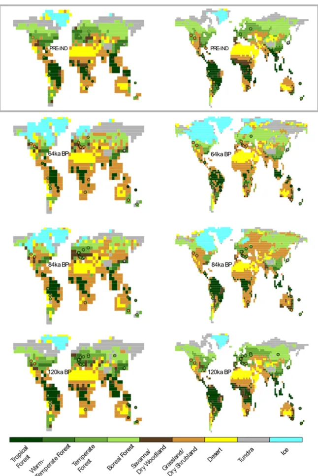
We present here an overview of the vegetation reconstruc-tions for the last glacial–interglacial cycle simulated in B4H and B4F. We compare the simulated biomes in B4H and B4F with each other and with the dominant megabiome rived from the pollen-based biomizations, restricting our de-scription of the results to major areas of agreement and dis-agreement. Maps of the dominant megabiomes produced by B4H and B4F with superimposed reconstructed dominant megabiomes for these periods are shown in Fig. 2.
We focus on a few specific periods, detailed below, since reviewing every detail present in this comparison is unfeasi-ble. The pre-industrial period serves as a test bed to identify biases inherent in our model setup, before climate anomalies have been added. The 6 ka BP mid-Holocene period repre-sents an orbital and ice-sheet configuration favouring gener-ally warm Northern Hemisphere climate (Berger and Loutre, 1991). The LGM simulation at 21 ka BP is at the height of the last glacial cycle, when ice sheets were at their fullest ex-tent, orbital insolation seasonality was similar to present and CO2 was at its lowest concentration (∼ 185 ppm), and the
resulting climate was cold and dry in most regions. These three time periods form the basis of the standard PMIP2 simulations and were used in the BIOME 6000 project. We thus additionally compare our simulations with the BIOME
6000 results for these time periods. The 54 ka BP interval is representative of peak warm conditions during Marine Iso-tope Stage 3 (MIS 3), where both the model climates and some proxy evidence suggest relatively warm conditions, at least for Europe (Voelker et al., 2002), associated with tem-porarily higher levels of greenhouse gases, an orbital con-figuration that favours warmer Northern Hemisphere sum-mers, and Northern Hemisphere ice sheet volume roughly half that of the LGM. The time slice 64 ka BP represents MIS 4, both greenhouse gases and Northern Hemisphere insola-tion were lower, and Northern Hemisphere ice volume was two-thirds higher than at 54 ka BP, resulting in significantly cooler global climate. The time slice 84 ka BP is representa-tive of stadial conditions of the early part of the glacial (at the end of MIS 5), after both global temperatures and atmo-spheric concentrations of CO2have fallen significantly and
the Laurentide ice sheet has expanded to a significant size but before the Fennoscandian ice sheet can have a major in-fluence on climate. The 84 ka BP period can be compared with the Eemian (120 ka BP, the earliest climate simulation used here), which represents the end of the last interglacial warmth (MIS 5e), before glacial inception. The Eemian pe-riod (120 ka BP) differs from the pre-industrial mainly in in-solation. The earlier parts of the Eemian (e.g. 125 ka BP) are often studied due to their higher temperature and sea level compared to the Holocene (Dutton and Lambeck, 2012), but 120 ka BP is the oldest point for which both FAMOUS and HadCM3 climates were available.
3.3.1 Pre-industrial
Our BIOME4 simulations were forced using anomalies from the pre-industrial climates produced by HadCM3 and FA-MOUS. Differences between B4H and B4F for this period thus only arise from the way the pre-industrial climate forc-ing has been interpolated onto the two different model grids we used. Differences between B4H and B4F and the pollen-based reconstructions for this period highlight biases that are not directly derived from climates of HadCM3 and FAMOUS but are inherent to BIOME4, the pollen-based reconstruction method, or simply the limitations of the models’ geographi-cal resolution.
Although few of the long pollen records synthesized in this study extend to the modern period and their geograph-ical coverage is sparse, a comparison with previous high-resolution biomizations of BIOME6000 (see Table 1 for de-tails; these studies include the sites synthesized here amongst many others) and Marchant et al. (2009) show that they are generally representative of the regionally dominant biome. The biomized records of Carp Lake and Lake Tulane in North America are exceptions, showing dry grassland con-ditions rather than the forests (conifer and warm mixed, re-spectively) that are more typical of their regions (Williams et al., 2000).
Figure 2.Reconstructed biomes (defined through highest affinity score) superimposed on simulated biomes using FAMOUS (B4F, left) and HadCM3 (B4H, right) climates for selected marine isotope stages (denoted in ka BP).
There is generally very good agreement between B4H and B4F for this period and the high-resolution BIOME6000 and Marchant et al. (2009) studies. A notable exception, common to both B4H and B4F, can be seen in the southwest USA being misclassified compared to the regional biomization of Thompson and Anderson (2000). The open-conifer wood-land biome they assign to sites in this region appears to be sparsely distributed (their Fig. 2) amongst larger areas likely to favour grassland and desert, and thus may be unrepresenta-tive of areas on the scale of the climate model grid boxes. The limitations of HadCM3 and FAMOUS’s spatial resolution appear most evident in South America, where the topographi-cally influenced mix of forest and grassland biomes found by Marchant et al. (2009) cannot be correctly reproduced, with disagreement at the grid-box scale between B4F and B4H. Eurasia is generally well reproduced, although the Asian bo-real forest biome does not extend far enough north, and over-runs what should be a broad band of steppe around 50◦N
on its southern boundary. Australia, with a strong gradient in climate from the coasts to the continental areas also shows the influence of the coarse model resolutions, with B4F more accurately reproducing the southern woodlands but neither simulation reproducing the full extent of the desert interior. Both Australian records are from the eastern coastal ranges; there are no long continuous records in the interior because of the very dry conditions. Overall, our comparison with the full BIOME6000 data set gives reasonable support to our working hypothesis that BIOME4, operating on the relatively coarse climate model grids we use here, is capable of produc-ing a realistic reconstruction of global biomes, although local differences may occur.
3.3.2 6 ka BP mid-Holocene
As for the pre-industrial period, in both the mid-Holocene and LGM periods the high-resolution biomizations of the BIOME6000 project (see Table 1) provide a better base for comparison of our model results than the relatively sparse, long time-series pollen records synthesized in this study. A common thread in the BIOME 6000 studies is the global similarity between the reconstructions for 6 ka BP and the pindustrial period, and this is, by and large, also the re-sult seen in B4H and B4F. An increase in vegetation on the northern boundary of the central Africa vegetation band is the most notable difference compared to the pre-industrial in the regional biomizations (Jolly et al., 1998), which is also sug-gested by the long central African pollen records synthesized here. Both climate model-based reconstructions show grass-land on the borders of pre-industrial desert areas in North Africa, although the additional amount of rainfall in both models is too low, and the model resolution insufficient to represent any significant “greening” of the desert. B4F shows a smaller change in tropical forest area in central Africa than B4H does, agreeing better with the regional biome recon-structions. Both HadCM3 and FAMOUS predict similar
pat-terns and changes in precipitation for this period, but the magnitude of the rainfall anomaly in FAMOUS is slightly lower. The reduction in forest biomes at the tip of South Africa in B4F has some support from Jolly et al. (1998), al-though B4F initially overestimates forest in this area.
B4H and B4F show limited changes elsewhere too. In North America, FAMOUS’s increase in rainfall anomalies produces more woodland in the west in B4F compared to the pre-industrial period, which is not seen in B4H. This is not a widespread difference shown in the regional biomization, although individual sites do change. Marchant et al. (2009) suggest drier biomes than the pre-industrial for some north-ern sites in Latin America, agreeing with B4F but not B4H. For Eurasia and into China, Prentice (1996), Tarasov et al. (2000), and Yu et al. (2000), all suggest greater areas of warmer forest biomes to the north and west across the whole continent, with less tundra in the north. However, nei-ther BIOME4 simulation shows these differences, with some additional grassland at the expense of forest on the south-ern boundary in B4H, and B4F predicting more tundra in the north. Although both FAMOUS and HadCM3 produce warmer summers for this period, in line with the increased seasonal insolation from the obliquity of the Earth’s orbit at this time, the colder winters they also predict for Eurasia skew annual average temperatures to a mild cooling which appears to prevent the additional forest growth to the north and west seen in the pollen-based reconstructions.
3.3.3 21 ka BP (Last Glacial Maximum)
For the LGM, both the BIOME4 simulations and pollen-data-based reconstructions predict a global increase in grass-lands at the expense of forest, with more tundra in north-ern Eurasia and desert area in the tropics than during the Holocene. Along with the cooler, drier climate, lower levels of atmospheric CO2also favour larger areas of these biomes.
Our long pollen records do not have sufficient spatial cover-age to fully describe these differences, showing only smaller areas of forest biomes in southern Europe, central Africa, and Australia, but there is again good general agreement between our two BIOME4 simulations and the regional biomizations of the BIOME6000 project.
The FAMOUS and HadCM3 grids do not seem to have sufficient resolution to reproduce much of the band of tun-dra directly around the Laurentide ice sheet in either B4H or B4F, but the forest biomes the simulations show for North America are largely supported by Williams et al. (2000). However, Thompson and Anderson (2000) suggest larger ar-eas of the open-conifer biome in the southwestern USA than in the Holocene that the BIOME4 simulations again do not show. Both B4H and B4F predict a smaller Amazon rainfor-est area. Marchant et al. (2009) suggrainfor-est that the Holocene rainforest was preceded by cooler forest biomes, whereas both HadCM3 and FAMOUS simulate climates that favours grasslands. Marchant et al. (2009) also provide evidence for
cool, dry grasslands in the south of the continent; FAMOUS follows this climatic trend but B4F suggests desert or tundra conditions, whilst B4H shows a smaller area of the desert biome. For Africa, Elenga et al. (2004) show widespread grassland areas where the Holocene has forest, with which the simulations agree, and dry woodland in the southeast, which neither B4H or B4F show; HadCM3 and FAMOUS appear to be too cold for BIOME4 to retain this biome. Elenga et al. (2000) also shows increased grassland area in southern Europe, which is not strongly indicated by either B4H or B4F, which have some degree of forest cover here.
The large areas of tundra shown by Tarasov et al. (2000) in northern Eurasia to the east of the Fennoscandian ice sheet are well reproduced by the BIOME4 simulations, al-though HadCM3’s slightly wetter conditions produce more of the boreal forest in the centre of the continent in B4H. The generally smaller amounts of forest cover in Europe in B4F agree with the distribution of tree populations in Eu-rope at the LGM proposed by Tzedakis et al. (2013) better than those from B4H, possibly due to HadCM3’s warm bias at the glacial maximum. Both B4H and B4F agree with the smaller areas of tropical forest in China and southeast Asia reconstructed by Yu et al. (2000) and Pickett et al. (2004) compared to the Holocene but have too much forest area in China compared to the biomization of Yu et al. (2000). Nei-ther BIOME4 simulation reproduces the reconstructed areas of xerophytic biomes in southern Australia, or the tropical forest in the north (Pickett et al., 2004).
3.3.4 54 ka BP (early Marine Isotope Stage 3)
There are fewer published biomization results for periods be-fore the LGM, so our model–data comparison is restricted to the pollen-based biomization results at sites synthesized in this paper. Of these sites, only two sites show a different megabiome affiliation when compared to the LGM: in South America, Uyuni shows highest affinity scores for the forest biome, and in Australia, Caledonia Fen shows highest affin-ity scores for the dry woodland biome (both sites show high-est affinity score for grassland during the LGM). Overall, the few sites where data are available show few differences com-pared with the LGM. This is perhaps a surprise given the ev-idence that this was a relatively warm interval within the last glacial, at least in Europe (Voelker et al., 2002). These mostly unchanged biome assignments derived from our pollen-data records are supported by our BIOME4 simulations in that, although both FAMOUS and HadCM3 do produce relatively warm anomalies compared to the LGM, both B4H and B4F simulations at 54 ka BP are similar to the LGM close to the pollen sites in the Americas, most of southern Europe (apart from Ioannina, where the data show highest affinity scores for temperate forest) and east Africa.
In other parts of the world, the biomes simulated at 54 ka BP in B4H and B4F do differ significantly from those of the LGM. Both BIOME4 simulations show increased
vege-tation in Europe and central Eurasia due to the climate in-fluenced by the smaller Fennoscandian ice sheet, as well as reduced desert areas in North Africa and Australia, gen-erally reflecting a warmer and wetter climate under higher CO2availability than at the LGM. However, our simulations
disagree on both the climate anomalies and the likely im-pact on the vegetation in several areas in this period. These include differences, both local and far-field, related to pre-scribed ice sheets, particularly in North America, where the ice-sheet configuration in FAMOUS shows largely separate Cordilleran and Laurentide ice sheets compared to the more uniform ice coverage of the continent in HadCM3. Further afield, B4H has significantly more tropical rainforest, espe-cially in Latin America, and predicts widespread boreal for-est cover right across Eurasia. B4F, however, reproduces a more limited forest extent, with more grassland in central Eurasia. The differences in the tropics appear to be linked to larger rainfall anomalies in HadCM3 than FAMOUS, whilst the west and interior of northern Eurasia is cooler in FA-MOUS than HadCM3. This may be due to the erroneously variable and low CO2applied to FAMOUS from the Vostok
record around this period, or it may indicate a stronger re-sponse to precessional forcing in FAMOUS, with a greater influence from the Fennoscandian ice sheet.
3.3.5 64 ka BP (Marine Isotope Stage 4)
There are only a few differences between biomized records at the LGM and 54 and 64 ka BP. Apart from one south-ern European site (Ioannina), which has a highest affilia-tion with grassland (compared with temperate forest during the LGM), the pollen biome affiliations are much the same as at the LGM for the sites presented here. The two sites in northern Australasia show a highest affiliation with the warm-temperate forest biome during this period, compared with tropical forest at 54 ka BP; however, affinity scores be-tween the two types are close, so this is unlikely to be related to different climates. The BIOME4 simulations support this as they also do not show major differences at the pollen sites. Both B4H and B4F are, in general, similar for 64 and 54 ka BP. The 64ka BP climate in HadCM3 is cooler and drier than for 54 ka BP, with B4H producing larger areas of tundra in north and east Eurasia and patchy tropical forests. There is less difference between 64 and 54 ka BP in the FAMOUS reconstructions, which simulates a cooler climate at 54 ka BP compared to HadCM3, so B4F and B4H agree better in this earlier period than at 54 ka BP. North American vegetation distributions primarily differ between B4H and B4F in this period due to the different configurations of the Laurentide ice sheet imposed on the climate models.
3.3.6 84 ka BP (Marine Isotope Stage 5b)
The pollen-based biomization for 84 ka BP clearly reflects the warmer and wetter conditions with more CO2available
than at 64 ka BP, especially in Europe, with the majority of sites showing highest affinity scores for the temperate forest biomes. Sites in other parts of the world show similar affin-ity scores to those at the 64 ka BP time slice, although there are not many sites and it is less clear whether they reflect widespread climatic conditions.
The BIOME4 simulations reflect the warmer European cli-mate resulting from the smaller Fennoscandian ice sheet at 84 ka BP than 64 ka BP, with B4F showing some European forest cover, and B4H extending Eurasian vegetation up to the Arctic coast. However, B4H shows more of this vegeta-tion to be grassland rather than forest, probably a result of a slightly cooler climate in HadCM3. Around the southern European pollen sites themselves, however, B4H shows little difference from the dry grassland biomes present at 64 ka BP and B4F predicts dry woodlands, perhaps a result of the mod-els’ representation of the Mediterranean storm tracks that would bring moisture inland which are often poorly repro-duced in lower-resolution models (Brayshaw et al., 2010).
Although there are differences in the configuration of the Laurentide ice sheet between HadCM3 and FAMOUS, both B4H and B4F reproduce dry vegetation types in the US Mid-west and significant boreal forest further north at 84 ka BP. Both BIOME4 simulations show significantly smaller desert areas in North Africa and larger areas of forest in the trop-ical belt than at 64 ka BP, reflecting significant precipitation and higher CO2levels here, although both also show a dry
anomaly over Latin America. Because of increased rainfall in Australia, B4H shows a smaller desert compared with 54 ka BP.
3.3.7 120 ka BP (last interglacial period, Marine Isotope Stage 5e)
This time slice represents the previous interglacial, and would be expected to have the smallest anomalies from the pre-industrial control climate of the climate models. The pollen-based biomization shows widespread forest cover for Eurasia, with the only other difference from both the 84 ka BP period and the pre-industrial control being Lake Titicaca, which has the highest affinity toward desert for this period. The affinity scores for temperate forest are almost as high for this site, and neither HadCM3 nor FAMOUS has the resolu-tion to reproduce the local climate for this altitude well (Bush et al., 2010), although both do reflect dry conditions near the coast here.
The models do indeed produce relatively small climate anomalies and vegetation similar to the pre-industrial con-trol and each other. Both models produce widespread forest cover north of 40◦N, much as for the pre-industrial climate, although FAMOUS is slightly too wet over North America for B4F to produce Midwest grasslands as seen in B4H. Both B4H and B4F increase the extent of their tropical forests, although FAMOUS has a relative dry anomaly over cen-tral Africa, and B4F has less tropical forest than for the
pre-industrial or B4H, which once again appears to have a stronger response to precessional forcing.
4 Global terrestrial vegetation changes
The BIOME4 simulations compare reasonably with biomiza-tions of BIOME 6000 (pre-industrial period, 6 ka BP, and LGM) and those presented in this paper. Below we calcu-late changes in the biome areas and net primary productiv-ity, keeping in mind that these calculations carry some un-certainties relating to several mismatches. As is discussed in Sect. 3.1 there are several occasions where the modern biomized pollen data do not agree with actual biome pres-ence, for example Potato Lake and Lake Tulane in North America. In both cases high contributions of Pinus and some other taxa skewed the affinity scores towards drier biomes (grassland and dry woodland). For the past, not knowing whether a pollen distribution is representative for an area puts restrictions on the biomization method. It is, however, noted that in most cases the biomized pre-industrial pollen agree with pre-industrial biomes. The climate models pro-duce some differences in climate forcing of the vegetation due to (1) difference in resolution, affecting the biome areal extent and altitude and (2) ice-sheet extent, affecting tem-perature (Sect. 3.2). We can use the pre-industrial period as a test bed to compare model outputs and pollen reconstruc-tions (using the BIOME 6000 database), showing that there are some biases that can be attributed to biases in BIOME4, some to the biomization method, and some to the models’ limiting geographical resolution.
4.1 Biome areas
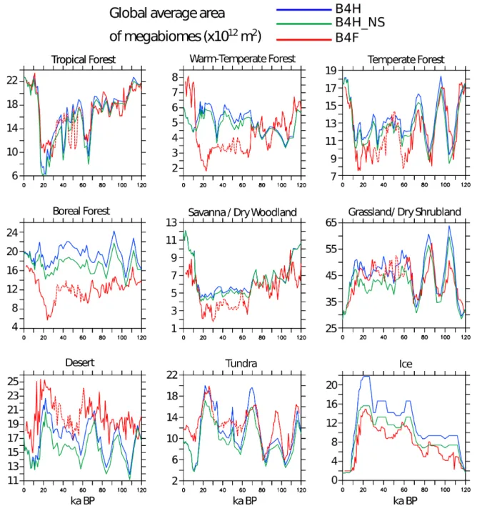
Whilst there is general agreement between B4H and B4F, there are also areas and periods with significant regional dif-ferences. A clearer picture of the effect on the global bio-sphere can be seen by using the global total areas of each megabiome for the two simulations (Fig. 3). Cooler temper-atures, reduced moisture, and lower levels of CO2 through
the glacial result in a general reduction of forest biomes and increases in grassland, desert, and tundra. Lower levels of atmospheric CO2also preferentially favour plants using the
C4 photosynthetic pathway (Ehleringer et al., 1997), con-tributing to the expansion of the grassland and desert biomes during the glacial. The changes in atmospheric CO2
lev-els through the glacial cycle are largely common to all the BIOME4 simulations, so CO2fertilization effects and C3/C4
competition are generally not responsible for differences in vegetation response between B4F and B4H. The exception to this rule comes between 40 and 60 kyr BP, where the FA-MOUS runs sees erroneously strong CO2variations in this
time interval from the Vostok record which may affect both the climate used to force B4F and the fertilization effects. B4F predicts consistently lower areas of warm-temperate and boreal forest than B4H, and higher amounts of grassland and
Figure 3.Global area coverage of megabiome types in the model reconstructions. S indicates the inclusion of potentially vegetated continen-tal shelves after sea level lowering, and NS indicates no vegetated continencontinen-tal shelves following sea level lowering. FAMOUS megabiome areas are represented by a dotted line between 30 and 60 ka BP in the period where the Vostok CO2data used to force the simulation is
thought to be erroneously low.
desert. FAMOUS also neglects the additional area of land that HadCM3 sees as continental shelves are exposed, re-ducing the area of land available to the biosphere, although some of this additional land is occupied by the Northern Hemisphere ice sheets in HadCM3. The global total areas of biomes highlights a significant oscillation in the areas of the different megabiomes of ∼ 20 kyr in length – this is par-ticularly notable between 60 and 120 ka BP in the grassland megabiome and results from the 23 kyr cycle in the preces-sion of the Earth’s orbit. The precespreces-sion cycle exerts a
signif-icant influence on the seasonality of the climate, as noted in tropical precipitation records (e.g. the East Asian monsoon; Wang et al., 2008; Carolin et al., 2013). Such variations are not explicitly evident in the dominant megabiome types at any of the pollen sites, but the precession oscillation does appear in the individual biome affinity scores of several sites (Supplement), lending support to this feature of the model reconstructions.