Defining clusters of related industries
The MIT Faculty has made this article openly available. Please share
how this access benefits you. Your story matters.
Citation Delgado, Mercedes; Porter, Michael E. and Stern, Scott. “Defining Clusters of Related Industries.” Journal of Economic Geography 16, no. 1 (June 2015): 1–38 © 2015 The Author(s)
As Published http://dx.doi.org/10.1093/jeg/lbv017
Publisher Oxford University Press
Version Original manuscript
Citable link http://hdl.handle.net/1721.1/109262
Terms of Use Creative Commons Attribution-Noncommercial-Share Alike
NBER WORKING PAPER SERIES
DEFINING CLUSTERS OF RELATED INDUSTRIES Mercedes Delgado
Michael E. Porter Scott Stern Working Paper 20375
http://www.nber.org/papers/w20375
NATIONAL BUREAU OF ECONOMIC RESEARCH 1050 Massachusetts Avenue
Cambridge, MA 02138 August 2014
This project has been funded by a grant from the Economic Development Administration of the U.S. Department of Commerce. We received financial support from Harvard Business School. We thank Bill Simpson, Xiang Ao, Rich Bryden, and Sam Zyontz for their invaluable assistance with the analysis. We also acknowledge the insightful comments of two anonymous reviewers, Harald Bathelt, Ed Feser, Frank Neffke, Juan Alcacer, Bill Kerr, Fiona Murray, Christian Ketels, James Delaney, Brandon Stewart, Muhammed Yildirim, Ram Mudambi, Sergiy Protsiv, Jorge Guzman, Sarah Jane Maxted and the participants in the Industry Studies Association Conference, NBER Productivity Seminar, Temple University Seminar, and the Symposium on the Use of Innovative Datasets for Regional Economic Research at George Washington University. The views expressed herein are those of the authors and do not necessarily reflect the views of the National Bureau of Economic Research.
At least one co-author has disclosed a financial relationship of potential relevance for this research. Further information is available online at http://www.nber.org/papers/w20375.ack
NBER working papers are circulated for discussion and comment purposes. They have not been peer-reviewed or been subject to the review by the NBER Board of Directors that accompanies official NBER publications.
© 2014 by Mercedes Delgado, Michael E. Porter, and Scott Stern. All rights reserved. Short sections of text, not to exceed two paragraphs, may be quoted without explicit permission provided that full credit, including © notice, is given to the source.
Defining Clusters of Related Industries
Mercedes Delgado, Michael E. Porter, and Scott Stern NBER Working Paper No. 20375
August 2014 JEL No. R0,R1
ABSTRACT
Clusters are geographic concentrations of industries related by knowledge, skills, inputs, demand, and/or other linkages. A growing body of empirical literature has shown the positive impact of clusters on regional and industry performance, including job creation, patenting, and new business formation. There is an increasing need for cluster-based data to support research, facilitate comparisons of clusters across regions, and support policymakers and practitioners in defining regional strategies. This paper develops a novel clustering algorithm that systematically generates and assesses sets of cluster definitions (i.e., groups of closely related industries). We implement the algorithm using 2009 data for U.S. industries (6-digit NAICS), and propose a new set of benchmark cluster definitions that incorporates measures of inter-industry linkages based on co-location patterns, input-output links, and similarities in labor occupations. We also illustrate the algorithm’s ability to compare alternative sets of cluster definitions by evaluating our new set against existing sets in the literature. We find that our proposed set outperforms other methods in capturing a wide range of inter-industry linkages, including grouping industries within the same 3-digit NAICS.
Mercedes Delgado
Temple University and ISC Fox School of Business Alter Hall 542 1801 Liacouras Walk Philadelphia, PA 19122 [email protected] Michael E. Porter Harvard University
Institute for Strategy and Competitiveness Ludcke House
Harvard Business School Soldiers Field Road Boston, MA 02163 [email protected]
Scott Stern
MIT Sloan School of Management 100 Main Street, E62-476
Cambridge, MA 02142 and NBER
2
1. Introduction
There is an increasing need for useful data tools to measure the cluster composition of regions, and support regional policy development as well as business strategy. The goal of this paper is to address this need by providing a rigorous methodology for generating and assessing sets of cluster definitions – groups of industries closely related by skill, technology, supply, demand, and/or other linkages. Our approach is novel by comparing the quality of alternative sets of cluster definitions and also by capturing multiple types of inter-industry linkages. We implement this clustering algorithm to create a new set of U.S. Benchmark Cluster Definitions (BCD), capturing a broad range of inter-industry linkages.
Clusters are geographic concentrations of related industries and associated institutions. The agglomeration of related economic activity is a central feature of economic geography (Marshall, 1920; Porter, 1990; Krugman, 1991; Ellison and Glaeser, 1997). Marshall (1920) highlighted three distinct drivers of agglomeration: input-output linkages, labor market pooling, and knowledge spillovers, which are associated with cost or productivity advantages to firms. Over time, an extensive literature has broadened the set of agglomeration drivers, including local demand conditions, specialized institutions, the organizational structure of regional business, and social networks (Porter, 1990, 1998; Saxenian, 1994; Storper, 1995; Markusen, 1996; Sorenson and Audia, 2000; among others). Thus, clusters contain a mix of industries related by various linkages (knowledge, skills, inputs, demand, and others) and supportive institutions.
The bulk of the cluster literature has been based on detailed case studies (Marshall, 1920; Porter, 1990, 1998; Swann, 1992; Saxenian, 1994). Over time, attention has begun to shift to larger-scale, quantitative studies across regions and industries (Porter, 2003; Feser, 2005). Using particular cluster definitions, studies have shown that the presence of related economic activity matters for regional and industry performance, including job creation, patenting, and new business formation (see among others, Feldman and Audretsch, 1999; Porter, 2003; Feser, Renski, and Goldstein, 2008; Glaeser and Kerr, 2009; Delgado, Porter, and Stern, 2010, 2014; Neffke, Henning, and Boschma, 2011).1 This evidence has informed key questions of both research and policy interest: the size of cluster effects, which mechanisms are most important in driving agglomeration, and how clusters diversify and grow in a region. Based on different
3
definitions of clusters, covering different portions of the economy ranging from high technological intensity industries to manufacturing to all industries defined in the industrial classification system, existing research has generated a range of results on these issues. However, the lack of a comprehensive methodology, and a way to compare alternative sets of cluster definitions, makes it difficult to reconcile key findings. This paper addresses this issue by developing a novel clustering algorithm to generate, assess and compare alternative sets of cluster definitions.
Cluster definitions are groups of industries related by skill, technology, supply, demand, and/or other linkages. This paper focuses on regionally comparable cluster definitions (i.e., the industries that constitute a cluster (e.g., Biopharmaceuticals) are the same for all regions). Inter-industry linkages are identified through the co-location patterns of industries across regions, or with a range of national data available across industries. The identified linkages are used to group industries into a set of defined clusters, allowing clusters to be compared across regions.
To generate a set of cluster definitions, we use clustering analysis – numerical methods for the classification of similar objects into groups (Everitt et al., 2011; Grimmer and King, 2011). Our algorithm generates many different cluster configurations, Cs, through a clustering function that utilizes a particular measure of the relatedness between any two industries and well-specified parameter choices (e.g., the number of groups). Each configuration is composed of mutually exclusive groups of related industries (i.e., clusters). The algorithm then provides scores that assess the quality of each C (i.e., its ability to capture meaningful inter-industry linkages within clusters). This allows us to identify the configuration, C*, that best captures
certain types of inter-industry links. Because an algorithm cannot perfectly substitute for expert judgment, the methodology concludes with an expert assessment and adjustment of individual clusters in C* to determine a final set of cluster definitions, C**.
Our paper contributes to the literature on clusters and economies of agglomeration in several ways. First, the clustering algorithm allows us to compare the quality of alternative sets of clusters using a common approach that generates objective scores (i.e., most clustering methods do not provide scores to help compare across groupings (Everitt et al., 2011; Grimmer and King, 2011)). We can assess cluster configurations that are generated using different inter-industry linkage measures. For example, we can evaluate Cs generated using pairwise inter-industry co-location patterns to those based on input-output or other measures. We can also compare
4
existing sets of cluster definitions. The ability to score sets of clusters can help identify the appropriate sets for addressing particular research and policy questions.
Our scoring approach utilizes a basic clustering principle: creating groupings so that industries within a cluster are more related to each other than to industries in other clusters based on various measures of inter-industry linkages. The score for a given C depends on how well it captures various types of industry linkages. However, what constitutes a useful set of cluster definitions may change depending on the particular research and policy question. Some studies may be interested in a particular type of industry link (e.g., labor occupational links), making sets of cluster definitions that perform better in that link more useful.
Second, our algorithm allows for experimentation with multiple inter-industry linkage measures used in the economies of agglomeration literature, including input-output linkages, occupational linkages, the co-location patterns of industries, and combinations among them. We can then examine the cluster configurations generated based on these different measures. The methodology can incorporate additional inter-industry linkage measures as they become available (e.g., a measure that specifically captures knowledge linkages), and score their resulting cluster sets.
Third, although generating cluster definitions will require expert judgment for some individual clusters, our algorithm is transparent. In the last stage of the algorithm, there is room for expert judgment to correct for inevitable anomalies that arise due to data imperfections and industry definitions. For example, in a given C*, there could be industry outliers that do not seem
to belong to their assigned cluster. These can be reallocated to their “next best” cluster using a score that assesses the relatedness of the particular industry with another cluster, using a transparent process. Users can assess how adjustments (re-allocations of industries, combining or dividing clusters) impact cluster scores.
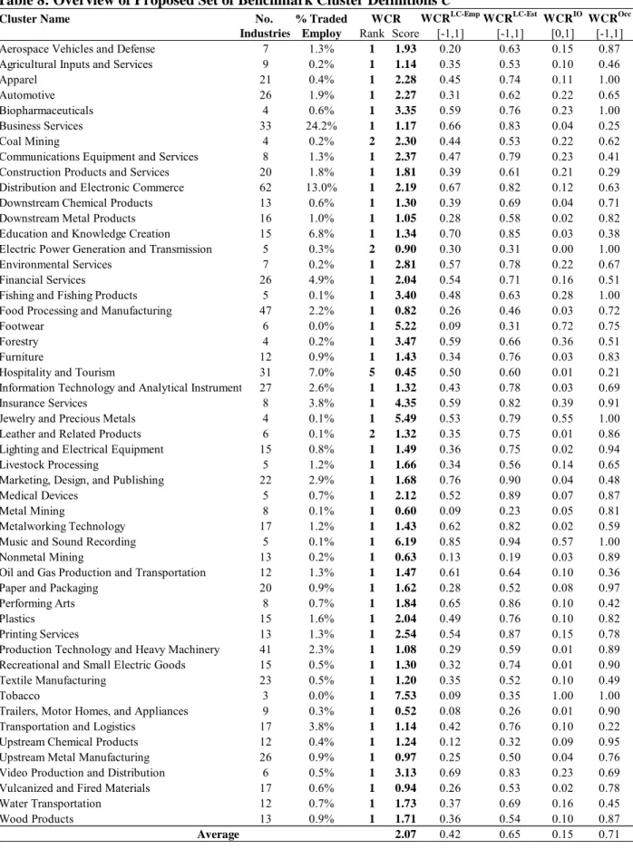
Another important contribution of this paper is that we implement our method to generate a new set of benchmark cluster definitions for the U.S. (BCD or C**), which captures a wide array of inter-industry linkages. The U.S.-based empirical analysis focuses on grouping 778 6-digit NAICS industries in manufacturing and services in 2009, and uses County Business Patterns (CBP), the Benchmark Input-Output Account of the United States, and Occupational Employment Statistics (OES) datasets to define multiple industry relatedness measures.
5
The proposed BCD is generated using inter-industry measures of co-location patterns of employment and the number of establishments, input-output links, and labor occupation links, and contains 51 clusters. We examine the relative performance of the BCD and three existing sets of (mutually exclusive) cluster definitions: industries within the same 3-digit NAICS, Porter (2003), and Feser (2005). Grouping industries within the same 3-digit NAICS scores poorly in capturing multiple inter-industry linkages, which is perhaps not surprising since the industrial classification system groups industries based on the similarities of their products/services, not on their inter-industry complementarities. Moreover, manufacturing and service industries belong to different parts of the NAICS, so that products and services are definitionally unrelated. Numerous empirical studies on economies of agglomeration have relied solely on industry codes to define inter-industry relatedness, potentially limiting their ability to capture a broad array of relevant industry linkages.
Our benchmark set scores higher in capturing a broader range of inter-industry linkages than the three other prominent sets of cluster definitions. The BCD also scores better or the same as the other sets in input-output linkages and shared labor occupations.
While the analysis is based on U.S. data, our clustering methodology can be implemented in other large and integrated economies with sufficient data availability. At present, however, U.S. data offers several advantages. Comparably large and diversified economic areas like the EU have heterogeneous data accessibility across countries, and current and past barriers to trade across locations can limit economies of agglomeration. Smaller economies (like the Nordics) have access to rich data, but their relative small size leads to specialization in a narrow range of industries.
Our benchmark cluster definitions offer a useful tool for research and policy on regional economic development. They allow the comparison of clusters across locations and over time by mapping the defined clusters into regional units and measuring the specialization patterns of regions in the clusters. Using the BCD, the U.S. Cluster Mapping Project has created a detailed regional cluster dataset that facilitates comparisons across regions and across clusters on numerous dimensions.2 For example, the Boston, MA and San Diego, CA Economic Areas have high employment specialization in Biopharmaceuticals, but the size and breadth of the cluster is
2 The U.S. Cluster Mapping website (http://clustermapping.us/) is supported by the U.S. Economic Development Administration, U.S. Department of Commerce.
6
lower in San Diego, which lacks specialization in biological products (except in-vitro diagnostic substances). The Project also includes data on the business environment and cluster institutions to inform research and policy. This data tool can be used in combination with cluster methods that focus on examining region-specific links among firms, individuals, and supportive institutions in clusters to shed light on the mechanisms at play in particular regional clusters.
The rest of the paper is organized as follows: Section 2 reviews the literature on industry cluster definitions. Section 3 describes our clustering algorithm. In Section 4, we discuss our main findings regarding the generation and assessment of cluster configurations, and Section 5 proposes a set of benchmark cluster definitions. In Section 6 we compare the BCD to existing sets of cluster definitions in the literature, and discuss some research and policy applications. Section 7 concludes.
2. Defining Industry Clusters
There are various types of economies of agglomeration identified in the literature, including input-output linkages, labor market pooling, knowledge spillovers, sophisticated local demand, specialized institutions, and the organizational structure of business and social networks (Marshall, 1920; Porter, 1990, 1998; Swann, 1992; Saxenian, 1994; Storper, 1995; Markusen, 1996; among others). These economies of agglomeration manifest themselves in clusters – geographic concentrations of related industries and associated institutions. Within regional clusters, firms and associated institutions (i.e., trade organizations, universities, and local government) can operate more efficiently and innovate faster due to sharing common technologies, infrastructure, pools of knowledge and skills, inputs, and responding to demanding local customers.
To implement cluster research and policy, however, we need to measure the boundaries of clusters: What set of related economic activity and institutions constitutes a cluster? Two main approaches to defining clusters have developed over the last 20 years: clusters based on inter-industry linkages inferred from multi-region analysis (which we refer to as comparable cluster
definitions) and cluster definitions based on observed linkages among industries or firms in a
single region (which we refer to as region-specific cluster definitions). Many empirically derived cluster definitions have been generated by researchers and practitioners over the years based on both approaches (see Cortright (2006) and Feser et al., (2009) for a review). The goal of this
7
paper is to develop a novel methodology to generate and assess sets of comparable cluster definitions. We next explain both approaches to define clusters and the contribution of our clustering method to the literature.
2.1 Comparable Cluster Definitions
A set of comparable cluster definitions allocates individual industries to specific clusters (e.g., Biopharmaceuticals), allowing clusters to be compared across locations. The defined clusters are mapped into regional units to measure the cluster specialization of regions. We can then compare particular clusters across regions, as well as the overall cluster composition of regions. Regional cluster strength reflects specialization in an array of related industries, not specialization in a narrowly defined single industry (Porter, 1998, 2003; Feldman and Audretsch, 1999; Delgado et al., 2014). Thus, regional cluster strength is conceptually similar to the notion of “related variety” introduced by Frenken et al. (2007). For example, a regional cluster with a high breadth of industries will capture related variety.
There are two types of inter-industry relatedness measures that have been developed in the literature (see Section 3.1 for a detailed explanation). Some studies use national-level data to capture particular inter-industry linkages, including knowledge links based on co-patenting (see e.g., Scherer, 1982; Koo, 2005a; Glaeser and Kerr, 2009); input and output links (see e.g., Feser and Bergman, 2000; Feser, 2005); skill links (see e.g., Koo, 2005b; Glaeser and Kerr, 2009; Neffke and Henning, 2013); and product similarity as defined by the industry classification system (e.g., same 3-digit NAICS). Still other studies define measures based on the co-location patterns of industries across many regions to capture various types of linkages (Ellison and Glaeser, 1997; Porter, 2003; Ellison et al., 2010). Only a few studies use the inter-industry relatedness measures to then define clusters of related industries. We next discuss the main existing sets of cluster definitions.
Knowledge Clusters. Studies of knowledge clusters focus on a selected set of U.S.
manufacturing industries with high technological intensity. For example, Feldman and Audretsch (1999) group industries that have a common science and technological base, using the Yale Survey of R&D Managers. This survey assesses the relevance of key academic disciplines for a product category. Industries with similar rankings of the importance of different academic disciplines are grouped into six mutually exclusive clusters. Alternatively, Koo (2005b) groups
8
manufacturing industries into seven mutually exclusive knowledge-based clusters using principal component factor analysis on an inter-industry patent-citation flow matrix.
Input-Output Clusters. Feser and Bergman (2000) define a set of U.S. manufacturing
clusters using input-output links based on the Benchmark Input-Output Accounts of the United States. They group input-output classification codes (IO codes) into 23 clusters using principal component factor analysis on an inter-industry input-output link matrix. The factor analysis method tends to create highly uneven clusters, with a large number of IO codes grouped into a few clusters. To address this issue, Feser (2005) develops a new methodology based on hierarchical clustering on an input-output link matrix for manufacturing and service activities. This transparent method creates a set of 45 mutually exclusive clusters. Overlapping clusters are then created in a second stage by identifying secondary IO codes highly related to the primary codes within a cluster. For each cluster, the method provides scores of the fit of each IO code within its cluster. The IO codes are then matched to 2002 NAICS codes to create a final set of clusters of related industries.
Co-Location-Based Clusters. Porter (2003) examines the co-location patterns of narrowly
defined industries in both service and manufacturing to define clusters, following the principle that co-location reveals the presence of linkages across industries. The methodology first distinguishes traded and local industries. Local industries are those that serve primarily the local markets (e.g., retail), whose employment is evenly distributed across regions in proportion to regional population. Traded industries are those that are more geographically concentrated and produce goods and services that are sold across regions and countries. The set of traded industries excludes natural-resource-based industries, whose location is tied to local resource availability (e.g., mining).
To measure the relatedness between a pair of traded industries (4-digit SIC), Porter (2003) computes the pairwise correlation of industry employment across states using 1996 data. This measure of co-location patterns is referred to as the “locational correlation” of employment (LC-Employment) and could capture various types of inter-industry linkages. Porter (2003) uses an iterative approach to define clusters rather than a clustering function approach. A set of 41 narrow (mutually exclusive) clusters are created using an iterative process to identify pairs and then groups of industries highly linked based on statistically significant locational correlations. In a second stage, a set of broad (overlapping) clusters is created by including other industries
9
that have a high locational correlation with the core industries within the narrow cluster. While the cluster definitions are mainly based on the empirical patterns of employment co-location among industries, the Benchmark Input-Output Account of the United States and industry definitions are used to correct the placement of industries with high co-location but low economic relatedness. These cluster definitions have proven very useful in the empirical analysis of the role of clusters on regional performance (see e.g., Porter, 2003; Delgado, Porter, and Stern, 2010, 2014).
2.2 Region-Specific Cluster Definitions
Comparable cluster definitions can capture most economic activities and are necessary for studies that aim to examine clusters across regions. However, one limitation of any multi-region cluster approach is that it may overlook specific inter-industry linkages that may exist in particular regional clusters. These idiosyncratic regional linkages are the focus of the region-specific cluster definitions. This approach focuses on a single region to measure industry and/or firm interdependencies and define the region’s clusters. Such studies vary in their industry coverage, types of economic units (industry, technology classes, or firms), types of regional units (administrative or non-administrative), and methods.
A small set of papers defines region-specific clusters for a large set of economic activities. Some of these studies identify specific “driver” industries in which a region has a competitive advantage. Then they use region-specific inter-industry linkages, such as regional input-output models, to define the clusters around the driver industries (Hill and Brennan, 2000). Other studies focus on identifying the (non-administrative) geographic boundaries of a given cluster. To do so, they examine the spatial density of businesses for particular industries (Duranton and Overman, 2005) or the spatial density of patents for particular technology classes (e.g., Kerr and Kominers, 2010; Alcacer and Zhao, 2013). The goal is to identify locations with a high density of economic activity in a particular field that will facilitate inter-firm connections and externalities.
The bulk of region-specific cluster definitions are qualitative and based on case studies that tend to focus on particular clusters (see e.g., Bresnahan and Gambardella (2004); Cortright, 2010; Porter and Ramirez-Vallejo, 2013), for example, the Athletic and Outdoor cluster in Portland (Cortright, 2010). These studies rely on existing cluster organizations, industry
10
directories, and other primary data collection to identify clusters. They offer rich details on the firms and institutions within particular defined clusters, but may be less appropriate for comparing clusters across regions.
The conceptual limitation to region-specific approaches to define clusters is that such definitions are based on observed linkages among existing economic activities in a region (Bathelt, Malmberg, and Maskell, 2004; Maskell and Malmberg, 2007; Feser et al., 2009; Bathelt and Li, 2013). Activities that are not present in a region (e.g., industries, technology classes, and labor occupations that are not present) are classified as unrelated to the other activities in the region. However, such non-present activities could be related to the activities in the region, but historical factors, market imperfections or other factors may have prevented their development. Region-specific cluster definitions could thus be too narrow (or myopic) in terms of the linkages captured because they abstract from the linkages that may be present in other locations. Thus, region-specific cluster definitions could be complemented by comparable cluster definitions derived from patterns across multiple regions.
This paper creates a new cluster methodology that systematically generates comparable cluster definitions based on multiple types of inter-industry linkages. This approach provides scores that assess the ability of each set of definitions to capture high inter-industry linkages within individual clusters. For example, we can compare the Feser (2005) and Porter (2003) sets of cluster definitions as well as other sets.
We implement the algorithm and propose a new set of U.S. Benchmark Cluster Definitions (BCD) that captures a wide variety of inter-industry linkages. This set can be updated over time as new data (e.g., new industry definitions) becomes available.
3. The Clustering Algorithm
In order to derive clusters of industries, we use cluster analysis, or numerical methods to classify similar objects (cities, people, genes, industries, etc.) into groups (Everitt et al., 2011). In contrast to network analysis, where each object is related to any other object,3 cluster analysis
3For example, some papers focus on defining the “product space” – the network of relatedness between products. Hidalgo et al. (2007) define the product space for exported goods. Other studies focus on specific dimensions of the product space, such as the technology, knowledge, or market space (Jaffe, Trajtenberg, and Henderson, 1993; Neffke et al., 2011; Bloom et al., 2012).
11
creates groups (termed clusters) in such a way that objects in the same cluster are more similar among themselves than to those in other clusters.
Defining clusters of related industries involves a number of key choices that can be parameterized in a clustering algorithm. The algorithm includes criteria for scoring alternative cluster configurations. Once the most promising configuration is identified, the algorithm addresses outlier industries to develop a final set of cluster definitions.
The clustering algorithm is designed to define mutually exclusive clusters, where each industry is uniquely assigned to one cluster. The methodology also allows the measurement of relatedness between any pair of (mutually exclusive) clusters and the creation of overlapping clusters (with individual industries shared by multiple clusters).
Drawing on Porter (2003), our method first distinguishes between traded industries (geographically concentrated) and local industries (geographically dispersed). There are 1,088 6-digit NAICS-2007 industries in the 2009 CBP data (excluding farming and some government activity). We identify 778 traded industries using the specialization and concentration patterns of each industry across U.S. regions. In 2009, the traded industries account for 36% of total U.S. employment, 50.5% of payroll, and more than 90% of patenting activity.4
The analysis focuses on grouping the 778 traded industries in service and manufacturing into non-overlapping groups. We refer to each cluster configuration as C and its individual clusters as c. There are five inter-related steps to create and assess each configuration C: (1) define a similarity matrix Mij that captures the relatedness between any two industries; (2) make
broad parameter choices β; (3) use a clustering function to create a configuration C based on the similarity matrix and parameter choices (C=F(Mij, β)); (4) calculate performance scores for each
C and identify the most promising configuration C*; and (5) assess and correct the individual
clusters in C* to determine the finalized set of cluster definitions C**. Each of these clustering
algorithm steps is explained in detail below.5
3.1 Step 1: Similarity Matrix
The first step to group related industries into clusters is to define the degree to which each pair of industries is related. A similarity matrix Mij provides the relatedness between any pair of
4 The complete description of the traded and local categorization can be found on the U.S. Cluster Mapping website. 5 All the steps of the algorithm were implemented using STATA software.
12
industries i and j. The matrix is based on the choice of indicator and the similarity measure. Indicators used in the literature include employment, number of establishments, measures of buyer-supplier linkages, and measures of shared labor requirements. The choice of a similarity measure allows the user to decide how the distance between two industries i and j should be measured (e.g., correlation coefficient, Euclidean, Jaccard index, or user-defined measures).
There are many alternative similarity matrices. Our analysis focuses on the inter-industry relatedness measures most frequently used in the field of regional studies to capture economies of agglomeration. The similarity matrices can be divided into three types. First, there are Mij that
exploit co-location patterns across many regions to capture various types of inter-industry linkages. This group includes the locational correlation of employment developed by Porter (2003) and the Ellison and Glaeser (1997) coagglomeration index. Second, there are Mij that
focus on national-level inter-industry linkages, including measures based on national input and output tables (see Feser and Bergman, 2000; Feser, 2005; Ellison, Glaeser, and Kerr, 2010) and on labor occupation links (Glaeser and Kerr, 2009). Third, we create multidimensional matrices that use a combination of these matrices. In what follows, we explain each of these similarity matrices as well as additional industry linkages we do not directly measure.
Pairwise Industry Co-location Patterns. Before we explain the co-location similarity
matrices used in our analysis, we need to clarify the regional unit used for these measures and the source of the underlying data. There are two spatial approaches to measure the co-location patterns of industries across regions: using discrete spatial units like states (Ellison and Glaeser, 1997; Porter, 2003; Ellison, Glaeser, and Kerr, 2010) and using continuous spatial units that are based on the density of businesses (Duranton and Overman, 2005). Discrete spatial units that capture relevant regional markets offer a reasonable starting point for understanding co-location patterns. The differences between discrete and continuous co-location measures in their ability to capture inter-industry externalities can be tested. For example, Ellison, Glaeser, and Kerr (2010) show that their co-agglomeration index based on states and an approximation of the continuous co-agglomeration metric developed by Duranton and Overman (2005) both capture similar inter-industry Marshallian effects (input-output, skill, and knowledge links). Using continuous spatial measures is beyond the scope of this paper due to data limitations.
We use meaningful administrative regional units: Economic Areas (EAs) as defined by the Bureau of Economic Analysis (BEA). EAs represent 179 relevant regional markets that cover
13
the entirety of the continental United States (Johnson and Kort, 2004). The underlying employment and count of establishments of an EA-industry is sourced from the County Business Patterns (CBP) 2009 data.6
Locational Correlation (LC). Porter (2003) examines the employment co-location
patterns of pairs of industries to capture inter-industry linkages of various types (e.g., technology, skills, supply, or demand links). He defines the locational correlation of employment (LC-Employment) of a pair of industries as the correlation coefficient between employment in industry i and employment in industry j in a region r:
(1).
Similarly, we also define an alternative locational correlation based on the count of establishments in a region-industry:
(2).
Economies of agglomeration channels include firms as well as employees. The presence of numerous establishments can facilitate inter-firm interactions that result in spillovers (Glaeser and Kerr, 2009). Thus, the co-location patterns of count of establishments could help capture inter-industry linkages that are facilitated by the number of businesses.
The correlation coefficient is a well-known distance measure for continuous data used in clustering analysis (Everitt et al., 2011). The LC measures can be implemented for very granular industry definitions, and its scale is easy to interpret, with values between -1 and 1. Positive and large values suggest that there are relevant economic interdependencies between a pair of industries. For example, if the location of employment (count of establishments) in electronic computers and software is highly correlated, it would suggest that both industries are linked. While the LC measures tend to capture relevant linkages, it is possible that in some cases industries with high co-location may have little economic relatedness but instead capture shared natural resources. As we discuss further below, this does not limit the usefulness of co-location measures.
LC also could be sensitive to the size of the regions (Porter, 2003). For example, for pairs
of industries with employment concentrated in large regions (i.e., with many pairs of zero
6 The CBP data is made available at the county, state, and U.S. level. Economic Area data is built up from the county file. CBP data uses cell suppression in certain geography-industries with a small presence of firms. When employment data is suppressed, a range is reported. We utilize the midpoint in the range in our data.
- ij ( ir, jr)
LC Employment Correlation Employment Employment
- ij ( ir, jr)
14
activity across regions), the LC could be biased. We limit this problem by using EAs versus using smaller regional units (like counties) that do not fully capture the regional market. We also implement several sensitivities to EA size that suggest this problem is limited.7 In our data, the average LC-Employment and LC-Establishments of a pair of industries are 0.30 and 0.52, respectively (Table 2).
The Coagglomeration Index (COI). This index developed by Ellison and Glaeser (1997)
captures whether two industries are more co-located than expected if their employment is distributed randomly. We use the revised version of the COI in Ellison, Glaeser, and Kerr (2010):
(3);
where sri is the share of industry i’s employment in region r; and xr measures the aggregate size
of region r, which they model as the mean employment share in the region across industries. A value of zero or negative for COI would suggest no externalities-driven co-agglomeration. The higher the positive value of the COI, the greater is the potential for externalities between two industries, but it is not easy to assess whether particular positive values are large or small.
Ellison et al. (2010) compute the COI for pairs of manufacturing industries (3-digit SIC codes) and use states as the main regional unit. They find that each of the three Marshallian effects (input-output, skill, and knowledge links) matter for the co-agglomeration of a pair of industries. However, shared natural advantages (e.g., coastal access) also matter for the co-agglomeration, but this effect is less important than the cumulative effect of the Marshallian factors. Their findings suggest that co-location captures not only meaningful economic interdependencies and externalities between industries, but also some natural advantages.
We extend the Ellison, Glaeser, and Kerr (2010) analysis, and compute the COI for 6-digit NAICS manufacturing and service industries, using EAs as the regional unit. The mean of this variable is around zero with a standard deviation of 0.010; and the values range from a minimum of -0.05 to a maximum of 0.37 (Table 2). These values are very similar to those obtained in Ellison et al. (2010) for 3-digit SIC manufacturing industries and with a state as the regional unit. In our data, the COI is skewed, with 90% of the distribution below 0.01.
7 We compute alternative LC matrices by dropping the 10 smallest and 10 largest EAs, and these LC matrices are highly correlated to our baseline measures based on all EAs.
2
ij ri r rj r r
r r
15
National-Level Inter-Industry Links. We explain the next two similarity matrices that are
based on national-level data: input-output and labor occupation links. Because these measures do not consider location patterns, they may capture industry interdependencies that are not geographically bounded.
Input-Output Links (IO). Measures based on the Benchmark Input-Output Accounts of
the United States are widely used to capture supplier and buyer flows between industries (see Feser, 2005; Ellison, Glaeser, and Kerr, 2010; Alcacer and Chung, 2012). Following Ellison et al. (2010), we construct a symmetric IO link between any pair of industries i,j based on the maximum of all unidirectional input and output links:
(4).
The inputij link is the share of industry i’s total value of inputs that comes from industry j, and the outputij link is the share of industry i’s total value of outputs that goes to industry j.
8 The
IOij link takes a minimum value of zero if the two industries do not buy from or sell to each
other, and a maximum value of 1 if any of the two industries buy or sell exclusively from or to the other.
To compute this variable, we use the 2002 Benchmark Input-Output Account of the United States developed by the BEA. The average of this variable is 0.02 (Table 2). Most pairwise industrial combinations have a small IO link (also documented at Ellison et al., 2010), making the distribution over all pairwise combinations skewed to the right. In our sample, 90% of the distribution of this variable is below 0.06. Overall, input-output tables are more detailed for manufacturing than service industries, and so may better capture links among manufacturing industries.9
In the sensitivity analysis, we also compute a more conservative IO link score that takes the average (versus maximum) of the unidirectional input and output links, correcting downwards the score for pairs of industries with large asymmetries in their links. The average
8 To properly capture the strength of the input-output links between two industries, we compute these percentages excluding final consumption and value-added commodity codes.
9 In the underlying input-output data, many manufacturing industries are only available at the 4/5-digit NAICS level, and many service industries at the 2/3-digit NAICS level. The following activities are aggregated at the 2-digit NAICS level: Construction (23 NAICS), Wholesale trade (42 NAICS), Retail trade (44 and 45 NAICS), and Management of Companies and Enterprises (55 NAICS). This higher level of aggregation may induce some measurement error in the links among the corresponding 6-digit NAICS industries (e.g., we have to assume that any 6-digit industries within Wholesale trade have the same input-output links with other 6-digit industries).
j j j
16
and maximum pairwise IO links are highly correlated, and our findings are robust to using these alternative measures.10
Labor Occupation Links (Occ). Labor occupations have been used to measure the extent
to which industries share similar skills (Koo, 2005a; Glaeser and Kerr, 2009). We use the Occupational Employment Statistics (OES) Survey of the Bureau of Labor Statistics (BLS; 2009 data). The OES data provides 792 non-governmental occupations and information on the prevalence of these occupations for each industry (i.e., for each occupation (e.g., computer programmers); it provides the percentage of that occupation in the total occupational employment of the industry). Using this data and following Glaeser and Kerr (2009), we compute the pairwise correlation between the occupation composition of any two industries:
(5);
where Occupationi is a vector with the percentage of each of the 792 occupations in the total
occupational employment of industry i. A limitation of this measure is that occupation data is aggregated at the 4-digit NAICS level (i.e., industries with the same 4-digit NAICS will have the maximum occupational link by construction).11 The average labor occupation correlation in our sample is 0.18.12
Multidimensional Similarity Matrices. We also create combinations of the
unidimensional similarity matrices described above. Creating multidimensional similarity matrices begins with understanding the relationship between the unidimensional matrices. Looking at the correlations in Table 3, Employment is highly correlated with
LC-Establishments (correlation of 0.77) and with the coagglomeration index (correlation of 0.36).
These high correlations are robust to the size of the industry and to manufacturing and service industries. IO links have a modest positive correlation with the other measures. We also explore a matrix that captures product similarity as defined by the industry code (NAICS-3). This matrix is equal to 1 for pairs of industries with the same 3-digit NAICS code (and 0 otherwise), and
10 Other papers use measures of indirect input-output links that capture the extent to which a pair of industries have meaningful suppliers and buyers in common (see Feser, 2005).
11 We are using 7-digit Standard Occupational Classification (SOC) and 4-digit NAICS data because of better coverage. The data can be accessed at http://www.bls.gov/oes/oes_dl.htm.
12 Another way to measure skill links between industries is to examine the actual flow of employment using matched employer-employee data for the workforce of a country. See Neffke and Henning (2013) inter-industry skill-relatedness analysis for the Swedish economy.
( , )
ij i j
17
relates very poorly with all similarity matrices except with occupational linkages (correlation of 0.45).
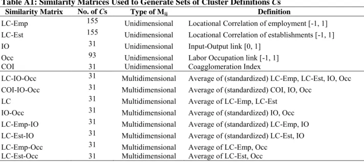
By using a multidimensional similarity matrix, we can better capture more types of inter-industry links (e.g., demand, supply, skills, knowledge, and others), and we can overcome some of the data limitations of the unidimensional matrices (see Table A1 in the Appendix for the definitions of all Mijused). For example, we compute an Mij that we call LC-IO-Occij, which is
the average of four (standardized) individual matrices: LC-Employmentij, LC-Establishmentsij,
IOij, and Occij.13 The multidimensional LC-IO-Occ has a high and statistically significant
correlation with each of the individual matrices (Table 3). This suggests that a pair of highly linked industries based on one particular measure (e.g., IO) will also tend to be meaningfully related based on the multidimensional similarity matrix. Thus, LC-IO-Occ seems to better capture various inter-industry links.
Through our algorithm, we can compare how well cluster configurations derived from different similarity matrices perform given the validation scores developed in Step 4 below. We can then assess which matrices seem to result in cluster configurations that capture the broadest range of inter-industry links (see Section 4).
Similarity Matrices and Alternative Agglomeration Mechanisms. While we explore a
particular set of relevant inter-industry measures, there are specific agglomeration mechanisms that we do not measure explicitly, such as knowledge linkages and social linkages.
Prior studies that focus on aggregated industries in manufacturing examine inter-industry knowledge linkages using patent citation patterns (e.g., Koo, 2005b; Ellison, Glaeser, and Kerr, 2010). We cannot create inter-industry patenting linkages due to data limitations.14 However, knowledge linkages may be partly captured by our industry linkage measures. For example, co-location patterns of industries could capture some knowledge links as shown by Ellison, Glaeser, and Kerr (2010). Two industries may co-locate across regions because they share knowledge, and proximity facilitates the flow of knowledge. Similarly, if two industries share labor occupations, knowledge linkages could flow more easily.
We also do not measure social linkages of firms and individuals, which are important to define regional clusters. The inter-industry economic links captured by our measures can
13 We standardize the unidimensional matrices since their scale and/or distribution are different (see Table 2). 14 We use narrowly defined industries (6-digit NAICS), making the bridge to patent classes noisy. Additionally, many service industries have low patent intensity.
18
facilitate opportunities for inter-firm interactions. For example, firms operating in industries that share labor requirements or other inputs are more likely to interact and develop socioeconomic links.
If measures of inter-industry knowledge linkages or social linkages become available, they could be incorporated into our clustering algorithm. We could compare them against other similarity matrices, and assess how cluster configurations that are generated using the new matrices perform in the validation scores defined in Step 4 below.
More broadly, the nature and intensity of knowledge and socioeconomic linkages can vary significantly across regional clusters. Studies of the network among firms, individuals, and associated institutions will be especially informative as to the mechanisms at work in specific clusters (Sorenson and Audia, 2000; Rosenthal and Strange, 2003; Feldman, Francis, and Bercovitz, 2005; Bathelt, Malmberg, and Maskell, 2004; Storper and Venables, 2004; Lorenzen and Mudambi, 2013).
3.2 Step 2: Broad Parameter Choices
The parameter choices (β) required as inputs to the clustering functions include setting the initial number of clusters (i.e., number of groups), determining how the underlying data should be normalized, and determining the starting values for the clustering function.
An important parameter choice in clustering analysis is the initial number of clusters (numc). There are 41 clusters in Porter (2003) and 45 input-output based clusters in Feser (2005). Current methods to identify the “optimal” number of clusters in clustering analysis are very inconclusive (Everitt et al., 2011). Therefore, we explore values for the number of clusters between 30 and 60. Overall, too few or too many groups could result in less useful cluster definitions. Too few clusters could result in large clusters that include industries that are not very related; and too many clusters could result in clusters that are not meaningfully different from each other. Using Step 4 in the cluster algorithm (described below), it is possible to compare the quality of different configurations based on differences in the initial number of clusters.
The other two parameter choices refer to the starting values and the type of normalization of the underlying data for the clustering functions. The starting values were chosen at random. The underlying data was either untransformed (raw) or row-standardized (rst). These two parameter choices are relevant only for partition-clustering functions: kmeans and kmedians. The
19
normalization of the data can be important for these two clustering functions since it could result in a better centroid for each individual cluster.15
3.3 Step 3: Clustering Function
Clustering functions are designed to find the greatest relatedness among industries within each cluster. There are several clustering functions F(•) for grouping industries into clusters (see Everitt et al., 2011; Grimmer and King, 2011). Each function creates a new grouping C based on the similarity matrix and parameter choices: C = F(Mij, β). Our analysis uses the main cluster
functions for continuous data: the hierarchical function (with Ward’s linkage) and centroid-based clustering functions (kmean and kmedian).16
Only hierarchical functions allow the user to import a particular similarity matrix. In contrast, kmean and kmedian functions require the underlying raw data to directly compute the similarity matrix (and centroids). Thus, for similarity matrices that require additional manipulation of the underlying data (e.g., IO or COI), we can only use the hierarchical function.
Example of Steps 1 to 3 of the Clustering Algorithm. To illustrate Steps 1 to 3 of our
algorithm, we replicate a set of cluster definitions that we already know, namely the 3-digit NAICS groupings. We define the similarity matrix NAICS-3ij as a symmetric binary matrix
where pairs of industries within the same 3-digit NAICS code are assigned a value of 1 (and a value of 0 otherwise). Then, we set the broad parameters (β) so that there are 66 clusters just as there are 66 different 3-digit NAICS codes for our 778 industries. Finally, we run the hierarchical clustering function using the NAICS-3 matrix and 66 clusters. As expected, we find that the resulting grouping C is indeed equal to the NAICS-3 groupings, validating the clustering algorithm.
3.4 Step 4: Performance Scores for Each C
Given the number of possible similarity matrices, parameters, and clustering functions that could be chosen, the number of alternative cluster configurations is quite large. By combining the choices described above in Steps 1 to 3 in different ways, we have generated 713
15 The centroid of a cluster is the mean industry employment (for kmean) and the median industry employment (for
kmedian). These centroids could be biased towards larger regional industries. To limit this problem, we allow for
row-standardization of the region-industry employment/establishment data.
16 We also tried hierarchical clustering with average linkages, but the resulting individual clusters were very uneven. See Grimmer and King (2011) for a new clustering approach that combines multiple clustering functions.
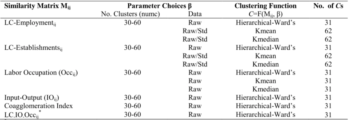
20
different Cs. For example, choosing the LC-Employment similarity matrix, 40 clusters, raw underlying data, and the kmean clustering function will result in one configuration C1.
Alternatively, choosing the IO links similarity matrix, 35 clusters, and the hierarchical clustering function will result in a different configuration C2 (see Table 1 for examples of Cs).
Without some way to evaluate the relative quality of all these Cs, it is very hard to find the most useful sets of definitions that incorporate a broad range of inter-industry linkages. The cluster analysis literature often lacks satisfactory methods for evaluating different categorization schemes (Grimmer and King, 2011). In contrast, our approach provides a score for each configuration C. In order to generate these scores, we must first address the question, What
makes a good set of cluster definitions?
In our analysis, the primary criterion for a good set of cluster definitions is that industries within a particular cluster (e.g., the Automotive cluster) should be more closely related among themselves than to industries in other clusters. In other words, individual clusters should be meaningfully different from each other, and individual industries should fit well within their own cluster. Our score approach assesses this by using alternative measures of inter-industry linkages that we use for creating validation sub-scores (e.g., sub-scores based on input-output links). Our view is that a useful set of clusters will capture various types of industry linkages, including demand, supply, skills, and others (Marshall, 1920; Porter, 1998). Thus, we develop an overall validation score (VS) for each C that combines sub-scores based on alternative industry measures.
A secondary criterion is that the configurations should be robust. We would prefer cluster definitions that are similar to other well-performing cluster definitions generated by the algorithm, since this would suggest that they are more robust. We develop Overlap Scores (OS) to capture the overlap of each C to other configurations.
Those Cs with the highest ranked validation scores are then subject to the robustness criteria to select the better configurations. The configuration that does relatively well in all criteria is the C* selected to undergo further assessment in Step 5. In the remainder of this section, we explain the validation and overlap scores.
Validation Scores. We develop validation scores that capture the extent to which
individual clusters and industries have high Within Cluster Relatedness (WCR) relative to Between Cluster Relatedness (BCR) with other clusters. The validation scores assess the quality
21
of a cluster configuration C along two dimensions. The first score, VS-Cluster, captures whether
individual clusters in C are meaningfully different from each other. The second score, VS-Industry, assesses the fit of individual industries within their own cluster. The two scores are
related, but capture different information. For example, in cluster configurations with many clusters, industries could fit very well in a cluster, but the individual clusters may not be very different from each other. Alternatively, in other cluster configurations with a few large clusters, individual clusters may be meaningfully different, but numerous industries may fit better in other clusters.
At the cluster level, we define WCRc as the average relatedness between pairs of industries within a cluster, while BCRc is the average relatedness between industries in cluster c and those in another cluster. For example, consider two clusters in C: cluster c1with industries
a1, a2and cluster c2 with industries b1, b2; and a similarity matrix Mij(e.g., LC-Employment) that
may be different from the one used to generate C. Then, the WCR of focal cluster c1 is
, and the BCR of c1 and c2 is .
For each focal cluster c in C, we compute its BCR with every other cluster and examine the resulting distribution to compute two cut-off values – the average and the 95th percentile values (AvgBCRc and Pctile95BCRc). For example, if there are 47 clusters in C, for each focal cluster c we then have 46 different BCRc values, and we compute the average and the 95th percentile of the BCRc values. We can then assess whether a cluster’s WCRc is higher than these two threshold values.
Once we define WCRc, AvgBCRc, and Pctile95BCRc for each cluster in C, we compute a validation score that captures the percent of clusters with high WCRc (VS-Cluster). This score is made up of two broad sub-scores that we average. The first calculates the percent of clusters in C with WCRc higher than AvgBCRc (VS-Cluster Avg) based on a particular similarity matrix Mij.
The second sub-score is similar but more restrictive; it calculates the percent of clusters in C with WCRc higher than Pctile95BCRc (VS-Cluster Pctile95):
(6a) (6b);
where Nc is the number of clusters in C and I is an indicator function equal to 1 if for a given
cluster c WCRc>AvgBCRc in (6a) or WCRc>Pctile95BCRc in (6b). We then average these two
1 1 2 c a a WCR M BCRc ,c1 2 Avg(M , M , M , M )a b1 1 a b1 2 a b2 1 a b2 2 M C c c ij c ij c
VS-Cluster Avg =(100/N )* I[WCR (M ) AvgBCR (M )]
M
C c c ij c ij
c
22
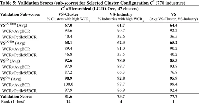
sub-scores to compute VS-ClusterM. For example, for C* the VS-ClusterLC-Emp score is 67.0%,
meaning that approximately 31 (of 47) clusters have relatively high WCRc based on
LC-Employment (Table 5).
We compute (6a) and (6b) based on four different Mij (Employment,
LC-Establishments, IO, and Occ). Note that the similarity matrices we use here are not dependent on
the similarity matrix used to create C. This allows us to calculate validation scores that can be consistently compared regardless of the underlying measures used to generate Cs. This results in eight sub-scores that we then average to generate the main validation score.17 A score of 100 indicates that all the individual clusters in C contain industries that are highly related based on multiple linkages. For example, for C* the VS-Cluster is 81.6% (Table 5), while the average of
this variable across all Cs is 73.9% (Table 4).
So far, we have computed a validation score that examines individual clusters. We then compute a validation score based on the fit of individual industries within their own cluster
(VS-Industry). For a given industry i, we want it to be more related to the industries within its own
cluster than to industries outside its cluster.18 Similar to our calculation of VS-Cluster, we measure the percent of industries with WCRic higher than their average BCRi (VS-Industry Avg) and higher than the 95th percentile of BCRi (VS-Industry Pctile95) based on various similarity matrices.
(7a) (7b);
where Ni is the number of industries in C. We compute (7a) and (7b) based on four different Mij
(LC-Employment, LC-Establishments, IO, and Occ), resulting in eight sub-scores that we then average to generate the validation score VS-Industry.
The overall validation score VS of a cluster configuration is computed as the average of the VS-Cluster and VS-Industry scores. Those Cs with highly ranked scores for both VS-Cluster
17 We do not include validation sub-scores based on COI to compute our main validation scores because COI and
LC-Employment will capture similar industry interdependencies.
18 The industry WCR
ic score is the average pairwise relatedness between the focal industry and the other industries within the cluster; while industry BCR is the average relatedness between the focal industry and industries in a different cluster. Using the example above, if we consider focal industry a1 in cluster c1, then its WCRa1c=Ma1,a2 and
the BCR of a1 with industries in cluster c2 is BCRa1, c2=Avg(Ma1,b1, Ma1,b2).
M
C i ic ij i ij
i
VS-Industry Avg =(100/N )* I[WCR (M ) AvgBCR (M )]
M
C i ic ij i ij
i
23
and VS-Industry are the most promising configurations (the “candidates” C*s). The final
candidate C* is the configuration with the maximum VS score. For example, Table 5 illustrates
the validation scores and sub-scores for the candidate configuration C*.
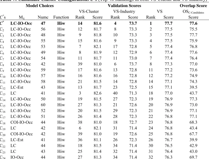
Overlap Scores. The candidate C*s are subject to the robustness criteria. We develop
scores that capture the robustness of a particular C by comparing the industry overlap between the clusters in C and the clusters in other candidate configurations. To compare a configuration
C1 to another C2, for each individual cluster c in C1, we find a matching cluster b in C2 (i.e., the
cluster b that has the highest industry overlap with c). Specifically, we compute the overlap between a pair of clusters c, b using the geometric mean of the industry overlap in each direction:
, 100 ( , / )
c b c b c b
overlap Shared Industries Industries Industries .
Where Shared Industries is the number of industries in common in b and c; and Industries are the number of industries in each cluster. The maximum overlap of a pair of matched clusters is 100. Then we define the overlap score of C1 to C2 as the average industry overlap across C1’s
clusters: 1 2 1 , 1 C C c b c C c
Overlap Score overlap
N
Similarly, we compute the average overlap of C1with all other candidate configurations (Overlap Score C-Candidates). For example, on average the
proposed candidate C* has an industry overlap of 77.6% with other relevant candidates,
indicating that these alternative Cs tend to provide, on average, similar groupings of industries (Table 7).
The configuration that does relatively well in the validation score (and overlap score) is the C* selected to undergo further assessment in Step 5. Generally, the higher the validation
scores, the better the C*. However, there could be anomalies within individual clusters that
would require some assessment and reallocation of individual industries to obtain the finalized set of cluster definitions C**.
3.5 Step 5: Assessing Individual Clusters of Candidate C*
Because clustering analysis cannot perfectly substitute for expert judgment, the methodology concludes with a systematic correction of anomalies and characterization of the individual clusters in C*, resulting in a finalized set of cluster definitions. Although Steps 1 to 4
systematically assign industries to clusters, the resulting Cs can be improved. Limitations in the underlying data may create spurious industry relatedness that will place some industries into
24
clusters where they are not the best fit. Some clusters may contain conceptually distinct groups that may have not been separated because of the choice of initial number of groups (numc parameter); and other clusters may be better off combined. Step 5 allows us to examine the clusters in C* to assess whether there are industry outliers that are better placed into different
clusters and whether to combine or break individual clusters to improve the coherence of the clusters. We can use our score approach to inform these expert-driven choices. Users can assess how certain changes impact the WCR scores of individual clusters and the validation scores of the cluster configuration relative to the initial values.
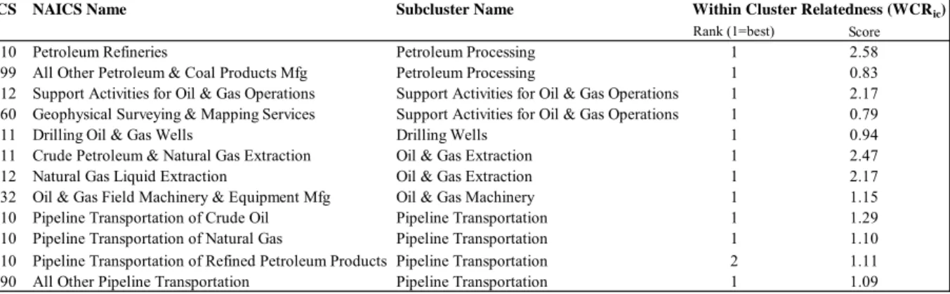
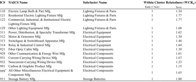
We define two types of possible outlier industries: systematic and marginal outliers. Systematic outlier industries are those with a low overall WCRic score (based on the average of standardized sub-scores for WCRLC-Emp, WCRLC-Est, WCRIO, and WCROcc).19 Systematic outliers are identified and corrected with a simple sub-process. They are identified based on two criteria: the industry WCR is low relative to other clusters (i.e., WCRic is below the 75th percentile value of BCRi); or WCR is low relative to other industries in the same cluster (i.e., WCRic is two standard deviations below the average WCRic). Then the systematic outliers are reassigned to the cluster where their WCR is highest. This sub-process is iterated several times until there are no systematic outliers.
Marginal outlier industries are those industries that, even with a high WCRic, could be conceptually better in another cluster. These outliers are often the result of limitations in the underlying data.20 For example, Men’s and Boy’s Clothing Manufacturing industries (NAICS 315221-31525) are in the Printing Services cluster for C*, but they likely best belong to an
Apparel cluster. Identifying these marginal outliers requires examining each cluster and analyzing the main product/service lines of the industries based on the detailed definitions offered by the NAICS system. The outliers are reallocated to their “next best” cluster using the
19 The WCR score is based on these four sub-scores to have a more robust score that captures multiple inter-industry linkages within the cluster.
20 In a few cases, the input-output link between two industries may be overestimated due to the level of aggregation of underlying data and/or due to our symmetric measure of IO links. For example, R&D industries (NAICS 541700) appear very highly linked to Water Transportation (NAICS 483000) industries because Water Transportation supplies a large percentage of its output to R&D industries. This induces the R&D industries to be grouped with Water Transportation if input-output links are considered in the similarity matrix. For industries where the underlying input-output data is highly aggregated and for industries with very high input-output links in the cluster, we check that these industries also fit well in their cluster based on the other measures (LC and Occ).
25
WCRi scores. Reallocated marginal outliers can be easily tracked and documented so that the process is transparent.
Once we correct industry outliers, we then examine whether some individual clusters should be combined or partitioned. If two individual clusters have very high BCR and they do not seem conceptually different, they could be combined. In contrast, some individual clusters could be partitioned if we find clear conceptual and relatedness differences among certain sub-groups of industries in a cluster. Because of these corrections, the initial number of clusters (numc) and the number of clusters in the finalized set of cluster definitions may differ.
After all five steps in the cluster algorithm are complete, we are able to recommend a final set of benchmark cluster definitions C** (the BCD). We explain the main findings and the
proposed new cluster definitions in the next Sections.
4. Generating and Assessing Cluster Configurations
We apply the clustering algorithm to generate 713 different cluster configurations that group 778 6-digit NAICS industries using 2009 U.S. data. These configurations are based on 13 different similarity matrices (Mij) and the parameter and clustering function choices discussed in
the prior section (C=F(Mij, β)). As illustrated in Table 1, some Cs are generated using
unidimensional matrices (e.g., Emp) and others using multidimensional matrices (e.g.,
LC-IO-Occ). We then generate the validation scores for each configuration to assess their relative
quality. In this section, we use the scores to compare Cs generated using different similarity matrices. We then explain the properties of the proposed candidate C* that will be subject to
assessment and adjustments of individual clusters in the last step of the algorithm to obtain the BCD.
Validation Scores by Choice of Similarity Matrix. Through our algorithm, we can
compare how well the configurations derived from different similarity matrices perform in the validation scores. We can then assess which similarity matrices seem to result in cluster configurations that capture the broadest range of inter-industry linkages and potential externalities (e.g., demand, supply, skills, knowledge, and others).
We use our score function to compare Cs generated by either a unidimensional similarity matrix (LC-Emp, LC-Est, COI, IO, Occ) or the multidimensional LC-IO-Occ matrix. Each of these matrices can be used to create a number of different Cs by changing the type of clustering