HAL Id: hal-01571232
https://hal.inria.fr/hal-01571232
Submitted on 1 Aug 2017
HAL is a multi-disciplinary open access
archive for the deposit and dissemination of
sci-entific research documents, whether they are
pub-lished or not. The documents may come from
teaching and research institutions in France or
abroad, or from public or private research centers.
L’archive ouverte pluridisciplinaire HAL, est
destinée au dépôt et à la diffusion de documents
scientifiques de niveau recherche, publiés ou non,
émanant des établissements d’enseignement et de
recherche français ou étrangers, des laboratoires
publics ou privés.
Maximum flow under proportional delay constraint
Pierre Bonami, Dorian Mazauric, Yann Vaxès
To cite this version:
Pierre Bonami, Dorian Mazauric, Yann Vaxès. Maximum flow under proportional delay constraint.
Theoretical Computer Science, Elsevier, 2017, 689, pp.58-66.
�10.1016/j.tcs.2017.05.034�.
�hal-01571232�
Maximum flow under proportional delay constraint
Pierre Bonamia,b, Dorian Mazaurica,c, Yann Vax`esaaAix-Marseille Universit´e, CNRS, LIF UMR 7279, 13000, Marseille, France. bIBM ILOG CPLEX, Madrid, Spain.
cInria Sophia Antipolis - M´editerran´ee
Abstract
Given a network and a set of source destination pairs (connections), we consider the problem of maximizing the sum of the flow under proportional delay constraints. In this paper, the delay for crossing a link is proportional to the total flow crossing this link. If a connection supports non-zero flow, then the sum of the delays along any path corresponding to that connection must be lower than a given bound. The constraints of delay are on-off constraints because if a connection carries zero flow, then there is no constraint for that connection. The difficulty of the problem comes from the choice of the connections supporting non-zero flow. We first prove a general approximation ratio using linear programming for a variant of the problem. We then prove a linear time 2-approximation algorithm when the network is a path. We finally show a Polynomial Time Approximation Scheme when the graph of intersections of the paths has bounded treewidth.
Keywords: Maximum flow, on-off delay constraints, polynomial time approximation scheme (PTAS), dynamic programming, bounded treewidth, linear programming.
1. Introduction
The multi-commodity flow problem is a classical network flow problem with multiple commodities (flow demands) between different source and sink nodes. This problem has been widely studied in the literature. Given a network, a set of capacities on edges, and a set of demands (commodities), the problem consists in finding a network flow satisfying all the demands and respecting capacities and flow conservation constraints. The integer version of the problem is NP-complete [6], even for only two commodities and unit capacities (making the problem Strongly NP-complete in this case). In that version, the problem consists of producing an integer flow satisfying all demands and respecting the previously mentioned constraints. However, if fractional flows are allowed, the problem can be solved in polynomial time through linear programming [1, 4, 8].
Network operators must satisfy some Quality of Service requirements for their clients. One of the most important parameters in telecommunications networks is the end-to-end delay of a unit of flow between a source node and a destination node. This requirement is not taken into account in the multi-commodity flow problem. The delay through a link depends on the amount of flow supported by this link; classically it is modeled by a convex function. The end-to-end delay for a demand and a path associated with this demand, is the sum of the delays through all links of this path. Some papers focus on minimizing the mean end-to-end delay. This problem consists of minimizing a convex function under linear constraints [3, 9] and can be solved using semidefinite programming [12]. Other papers focus on finding a multi-commodity flow that satisfies the demands and that minimizes the maximum end-to-end delay [5].
As the authors of [2], we think that a more realistic problem consists of adding strict end-to-end delay constraints for all connections. Indeed, in communication networks, there are multiple classes of services, and for each of them, it is crucial to respect a certain level of Quality of Service, i.e. respecting a threshold for the end-to-end delay. It is why we study a multicommodity flow problem in which all demands have to respect an end-to-end delay constraint.
In this paper, we focus on multicommodity network flow problems in which each edge possesses a proportional latency function that describes the common delay experienced by the flow on that edge as a function of the flow rate. These problems model congestion effects that appear in a variety of applications such as communication networks, vehicular traffic, supply chain management, or evacuation planning. In such applications, the latency function need
not be proportional to the flow rate. We investigate the problem of maximizing the sum of the flow under proportional delay constraints. We allow fractional flows for all connections. As mentioned before, we have an end-to-end delay constraint for each demand. But, if a path associated with one connection carries zero flow, then the constraint is not active. These on-off constraints make the problem more difficult to solve than just a simple linear program [7].
In [2], it is proved that this problem is NP-hard even if there are only two paths per connection. In their proof, delay and capacity constraints are used. The complexity of the problem is unknown when only considering delay constraints. We formally present our problem in Section 1.1. We then describe a simple example in Section 1.2 and preliminary results in Section 1.3. We present our contributions in Section 1.4.
1.1. Problem formulation and model
Let G = (V, E) be a connected undirected graph (that represents a network) with a coefficient αefor each edge
e∈ E. Let {(s1,t1), . . . , (sm,tm)} be a set of m source destination pairs (connections). Let
P
= {P1, . . . , Pm} be a set ofmpaths in G. For all i = 1, . . . , m, Piis the path, between the source siand the destination ti, allocated to connection
(si,ti). Without loss of generality, we suppose that there is a unique path for each connection. Indeed, we can have
several connections involving the same pair of nodes but with different associated paths. We denote by xi the flow
through the path Pifor all i = 1, . . . , m. We suppose that the delay τefor crossing an edge e ∈ E is proportional to the
total flow ∑i:e∈E(Pi)xicrossing the edge e, i.e. τe= αe∑i:e∈E(Pi)xi. Let λ> 0. For all i = 1, . . . , m, we require for path
Pithat, if xi> 0, then the end-to-end delay ∑e∈Piτeis at most λ. By scaling the coefficients of the αe, we can make
this bound λ equal to one. Using the notation βi, j:= ∑e∈E(Pi)∩E(Pj)αe, these constraints can be written as follows:
∑mi=1βi, jxi≤ 1. A multicommodity flow x = (x1, . . . , xm) is admissible if the following latency requirement is satisfied:
for all j = 1, . . . , m such that xj> 0, then ∑e∈E(Pj)τe≤ 1. Furthermore, for all i = 1, . . . , m, if xi> 0, then we say that
connection (si,ti) and path Piare active (inactive otherwise). The Maximum Flow under Delay Constraint problem
(FDC) consists in finding among the solutions satisfying these constraints a solution of maximum value ∑mi=1xi, i.e.:
Max ∑mi=1xi ∑mi=1βi, jxi≤ 1 j= 1, . . . , m xj> 0 xi≥ 0 i= 1, . . . , m.
The hardness of this problem comes from the choice of the active paths. Indeed, if we are given a set of active paths
P
∗⊆P
in some optimal solution, then the problem becomes polynomial since it reduces to solving the linear programLP(
P
∗). Without loss of generality letP
∗= {P1, . . . , Pm∗} with m∗≤ m. LP(
P
∗) Max ∑m ∗ i=1xi ∑m ∗ i=1βi, jxi≤ 1 j= 1, . . . , m∗ xi≥ 0 i= 1, . . . , m∗.The dual of this linear program is:
DLP(
P
∗) Min ∑m ∗ j=1yj ∑m ∗ j=1βi, jyj≥ 1 i= 1, . . . , m∗ yj≥ 0 j= 1, . . . , m∗. Note that LP(P
∗) and its dual DLP(
P
∗) differ only by the sense of inequalities and the direction of optimization. In particular, if the system of equations ∑mi=1∗ βi, jxi= 1, j = 1, . . . , m∗, has a solution then this solution is optimal for the
primal and for the dual since it satisfies both primal and dual complementary slackness conditions. 1.2. Example
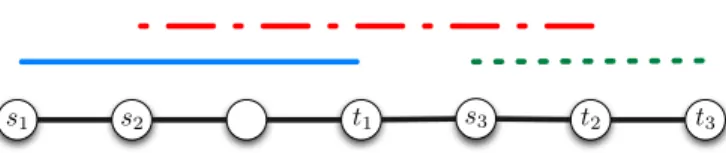
Consider the path G = (V, E) described in Figure 1 and the three source destination pairs (s1,t1), (s2,t2), and
(s3,t3). We set αe= 1 for all e ∈ E. FDC consists of solving:
Max x1+ x2+ x3 x1(3x1+ 2x2) ≤ x1 x2(2x1+ 4x2+ x3) ≤ x2 x3(x2+ 2x3) ≤ x3 x1, x2, x3≥ 0
s2
s1 t1 s3 t2 t3
Figure 1: Instance of FDC: path G = (V, E) with αe= 1 for all e ∈ E, and three source destination pairs (s1,t1), (s2,t2), and (s3,t3).
The first constraint means that, if the path P1is active, then the end-to-end delay for connection (s1,t1) must be at
most one. The delay for crossing the leftmost edge of P1is x1. The delay is x1+ x2for each of the two other edges.
Thus, if x1> 0, then 3x1+ 2x2≤ 1. Note that if x1= 0, the first constraint is always satisfied. The second and the
third inequalities are constructed similarly. One can observe that x∗= (1/3, 0, 1/2) is the optimal solution. Note that connection (s2,t2) is inactive, i.e. x2= 0, and so the second constraint is satisfied. That explains why the end-to-end
delay 2x1+ 4x2+ x3= 7/6 > 1 for connection (s2,t2) is not satisfied.
1.3. Preliminaries
We first prove in Lemma 1 that we can consider instances such that the path of a connection is not included in a path of another connection (but the paths may intersect).
Lemma 1. Let I be an instance of FDC. If there are two different connections Pjand Pksuch that E(Pk) ⊆ E(Pj), then
there is an optimal solution x∗such that x∗j= 0.
Proof. Consider any admissible flow x for I such that xj> 0. We construct another admissible flow x0from x in which
we only change the amount of flow for paths Pjand Pk. More precisely, we set x0k:= xk+ xj, x0j:= 0, and x 0
i:= xifor
all i ∈ {1, . . . , m} \ { j, k}. Clearly, the total amount of flow is unchanged, i.e. ∑m
i=1xi= ∑mi=1x0i. Let τ and τ
0denote the
vector of delay for x and x0, respectively. By construction of x0, we get τ0e≤ τefor all e ∈ E because E(Pk) ⊆ E(Pj). As
xis an admissible flow, then it follows that ∑e∈E(Pi)τ
0
e≤ 1, for all i = 1, . . . , m. Thus, the vector of flow x0is admissible.
To conclude, if x is an optimal solution, then x0is an optimal solution such that x0j= 0.
By Lemma 1, we only consider instances such that E(Pk) 6⊆ E(Pj) for all j, k ∈ {1, . . . , m}, j 6= k.
Let us define the graph H of intersections of the paths of an instance of FDC. The set of nodes V (H) = {h1, . . . , hm}
corresponds to the set of paths
P
= {P1, . . . , Pm}. For i, j ∈ {1, . . . , m}, i 6= j, there is an edge {hi, hj} ∈ E(H) betweentwo nodes hi∈ V (H) and hj∈ V (H) if, and only if, there exists e ∈ E such that e ∈ E(Pi) ∩ E(Pj), i.e. when Piand
Pj share at least one edge. The graph H of intersections of the paths of the instance depicted in Figure 1 is a path
composed of three nodes. Without loss of generality, we assume that the graph H is connected. Indeed, if H is not connected, we can consider the maximal connected components of H as independent instances of FDC.
1.4. Contributions
The complexity of FDC is still unknown but we conjecture that it is very hard to solve even for simple classes of instances. In this context, we make the following contributions. In Section 2, we prove a general polynomial approximation algorithm and a polynomial L-approximation algorithm, where L is the size of a longest path of
P
. In Section 3, we prove a linear time 2-approximation algorithm when G is a path. In Section 4, we prove a Polynomial Time Approximation Scheme (PTAS) when the graph H of intersections of the paths has bounded treewidth.2. Approximation algorithms using linear programming
This section is dedicated to prove approximation algorithms for FDC based on a variant of the problem, called Maximum Flow under Strong Delay Constraint problem (FSDC), for which all the end-to-end delay constraints must be satisfied even for inactive connections. This problem is polynomial since it reduces to solving the linear program LP(
P
), i.e. LP(P
∗) previously described when replacingP
∗byP
and m∗ by m. Note that an admissible solutionfor FSDC is an admissible solution for FDC because the end-to-end delay constraints are satisfied for all (active and inactive) connections in FSDC. Consider the example of Figure 1. One can observe that x = (1/4, 0, 1/2) is an optimal
solution for this variant of the problem. Such a solution for FSDC obtained by solving LP(
P
) is close to the optimal solution x∗for FDC. Indeed, (x∗1+ x∗2+ x∗3)/(x1+ x2+ x3) = 10/9.We first analyze the ratio between the value of an optimal solution for FSDC and the value of an optimal solution for FDC. We then deduce some polynomial approximation algorithms for FDC based on the solution of the linear program LP(
P
) for FSDC (Theorem 3 and Corollary 1). Let us first define some parameters and prove Lemma 2. Definition 1. For all k = 1, . . . , m, let S∗k⊆ {1, . . . , m} \ {k} be a maximum cardinality set of indices such that for all
i∈ S∗
k, there exists e ∈ E(Pk) ∩ E(Pi) such that for all j ∈ S ∗
k\ {i}, e /∈ E(Pj). Let |S
∗| = max
i=1,...,m|S∗i|.
Intuitively, S∗k is a maximal set of (indices of) paths that each have a ”private” edge in common with Pk(i.e. an
edge not shared with another path).
Lemma 2. Let I be any instance. Let x∗be an optimal solution for FDC and let x be an optimal solution for FSDC. Then ∑mi=1xi≥ ∑mi=1xi∗/|S
∗|.
Proof. Recall that if x∗k> 0, then ∑e∈E(Pk)τ∗e≤ 1. We first prove that if xk∗= 0, then ∑e∈E(Pk)τ∗e≤ |S∗k|. Let Pkbe a path
such that x∗k= 0. Consider a minimal (by inclusion) set of active paths S ⊆
P
that covers all edges of Pksupportingnon-zero flow. By definition of S∗k, |S| ≤ |S∗k|. Assign to each edge e ∈ E(Pk) supporting non-zero flow, a path Pi, i ∈ S
such that e ∈ Pi. For each i ∈ S, let Eibe the set of edges assigned to the path Pi. Since x∗i > 0, ∑e∈Eiτ
∗
e≤ 1, i.e. the
sum of the delays on the edges of Eiis at most 1. There are |S| groups of edges, and thus ∑e∈E(Pk)τ
∗
e≤ |S| ≤ |S∗k|, i.e.
the total delays on the edges of Pkis at most |S∗k|.
For all k ∈ {1, . . . , m} such that x∗
k= 0, then ∑e∈E(Pk)τ
∗
e≤ |S∗k|. Consider the solution x
0obtained by dividing all the
flows of x∗by |S∗|. Formally, set x0
i:= x∗i/|S∗| for all i = 1, . . . , m. By construction, ∑mi=1x0i= ∑mi=1x∗i/|S∗|. By previous
claims, x0is an admissible solution for FSDC. Finally, an optimal solution x for FSDC satisfies ∑mi=1xi≥ ∑mi=1x0i.
Because FSDC is polynomial and by Lemma 2, we deduce the following theorem: Theorem 3. There exists a polynomial |S∗|-approximation algorithm for FDC.
Let k ∈ {1, . . . , m} such that |E(Pi)| = L, where L = maxi=1,...,m|E(Pi)| be the size of a longest path. By definition,
Sk∗is a maximal set of paths for which there exists at least one edge that is not shared with another path (of S∗k). We get that |S∗| ≤ L. Indeed, the number of ”private” edges cannot be greater than the number of edges of the path. We deduce the following corollary of Theorem 3:
Corollary 1. There exists a polynomial L-approximation algorithm for FDC, where L = maxi=1,...,m|E(Pi)|.
Finally, when the graph G is a path, one can observe that |S∗| ≤ 2. Indeed, by Lemma 1, we assume that any path (of a connection) is not included in another path, and so S∗k is composed of at most two paths (”located” in both extremities) for every k ∈ {1, . . . , m}. Thus, there is a polynomial 2-approximation algorithm. For such class of instances, we prove in Section 3 a stronger result (in terms of complexity), namely a linear 2-approximation algorithm for FDC.
3. Linear time 2-approximation algorithm when G is a path
This section is dedicating to proving another polynomial 2-approximation algorithm when the graph is a path. The interest of this algorithm is its linear time complexity. A solution x of FDC is said to be independent if its support {Pk: xk> 0} is a family of edge-disjoint paths. In other words, x is independent if the set of vertices {hk: xk> 0} ⊂ V (H)
forms an independent set of H. Recall that the graph H is the graph of intersections of the paths. We prove in Lemma 4 that a best independent solution has a value which is at least half the total flow of an optimal solution if G is a path. Note that x = (1/3, 0, 1/2) is the best independent solution for the instance depicted in Figure 1 (that coincides in that case to the optimal solution of FDC). In the following, we consider that H is node-weighted. For all i = 1, . . . , m, the weight whi(or simply denoted wi) of the node hi∈ V (H) represents the maximum amount of flow that can support the
Lemma 4. Let I be any instance and let G be any path. Let x∗be an optimal solution and let x be a best independent solution for FDC. Then ∑mi=1xi≥12∑mi=1x∗i. There exists a linear time2-approximation algorithm for FDC when G is
a path.
Proof. Consider an optimal solution x∗of an instance I and the instance I0 obtained from I by removing all source-destination pairs that do not belong to the support of x∗. Since instances I and I0 have the same optimum and an independent solution for I0is also an independent solution for I, it suffices to prove the claim of lemma 4 for I0. For the instance I0, there is an optimal solution in which all delay constraints are active. This solution is therefore an optimal solution of the linear program LP(
P
∗) where
P
∗:= {Pi: x∗i > 0} and its value is at most the value of any feasible
dual solution y of DLP(
P
∗). Without loss of generality let
P
∗= {P1, . . . , Pm∗} with m∗≤ m. Let xI0 be an optimal
independent solution of I0, we will show that there exists a feasible solution yI0 of DLP(
P
∗) whose value is at mosttwice the value of xI0.
Since G is a path, the graph H of intersections of the paths is an interval graph. Let
C
be the set of maximal cliques of H. Since H is perfect, from the theory of perfect graphs (see for instance Chapter 65 of [11]), the caracter-istic vector z of a maximum weighted independent set is an optimal solution of the following linear program LPQ(P
∗):(LPQ(
P
∗)) Max ∑m ∗ i=1wizi ∑i:hi∈Czi≤ 1 ∀C ∈C
zi≥ 0 i= 1, . . . , m∗.Consider the dual (DLPQ(
P
∗)) of this linear program :(DLPQ(
P
∗)) Min ∑C∈CtC ∑C:hi∈CtC≥ wi i= 1, . . . , m ∗ tC≥ 0 ∀C ∈C
.Let t be an optimal solution of DLPQ(
P
∗). The following algorithm computes from t, a feasible solution y of DLP(P
∗).Let C ∈
C
, we denote l(C) (resp. r(C)) the index of the leftmost (resp. rightmost) path such that its corresponding node in H belongs to the clique C. For all i = 1, . . . , m∗ do yi := 0, and for all C ∈C
do yl(C):= yl(C)+ tC andyr(C):= yr(C)+ tC. Since the value of each variable tCfor C ∈
C
is added to exactly two variables yj, j = 1, . . . , m∗, thevalue of y is at most twice the value of t. For all i = 1, . . . , m∗, if e ∈ E(P
i) the following inequality holds: ∑j:e∈E(Pj)yj≥ ∑C:hi∈CtC≥ wi. Since t is a feasible
solution of DLPQ(
P
∗), the second inequality is trivially true. In order to verify the first inequality, note that if thenode hicorresponding to the path Pibelongs to the clique C then e ∈ E(Pi) implies that e ∈ E(Pl(C)) or e ∈ E(Pr(C)).
Thus, if a clique C contributes tC for the second sum then yl(C)or yr(C)contribubes tC for the first one. We conclude
that, for all paths i = 1, . . . , m∗, ∑e∈E(Pi)αe(∑j:e∈E(Pj)yj) ≥ ∑e∈E(Pi)αewi= wi∑e∈E(Pi)αe= 1.
This shows that y is a feasible solution of DLP(
P
∗). By the definition of y, its value is at most twice the weight ofa maximum weight stable set S of H. The independent solution corresponding to S is thus a 2-approximation for the instance I0.
To conclude the proof, computing an optimal independent solution when G is a path reduces to compute a maxi-mum weighted independent set of H and so we get the linear time complexity because H is an interval graph.
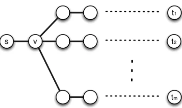
Note that we cannot find a similar result when the graph G is a tree. Indeed, a best independent solution may be arbitrarily far from an optimal solution for this class of graphs. As an example, consider the instance depicted in Figure 2. The graph G is a tree composed of m edge disjoint paths between v and the leaves ti, 1 ≤ i ≤ m, each
composed of m edges, and there is an edge between s and v. There are m ≥ 1 source destination pairs (s,t1), . . . , (s,tm).
For every i ∈ {1, . . . , m}, we denote by Pithe path corresponding to connection (s,ti). For every edge e ∈ E \ {s, v},
then αe= 1, and αs,v= 1/m. Since {s, v} ∈ E(Pi) for every i ∈ {1, . . . , m}, then any independent solution contains at
most one active path and the total amount of flow is at most m/(m2+ 1). Furthermore, if x
i= 1/(1 + m) for every
i∈ {1, . . . , m}, then x is an admissible solution for FDC such that the total amount of flow is m/(1 + m).
Conjecture 1. Let k ≥ 1 be any constant integer and let Hkbe the node-weighted graph constructed as follows. The set of vertices is the family of all the subsets of at most k paths (connections), and there is an edge between two nodes u and v if, and only if, there is at least one edge of G that belongs to one path of u and to one path of v. The weight
s v t2
t1
tm
Figure 2: Instance of FDC such that a best independent solution is arbitrarily far from an optimal solution. See details in the text.
e c b a f d a,b,c b,c,e c,e,f b,e,d u1 u2 u3 u4
Figure 3: A graph H of intersections of the paths (left) and an optimal tree decomposition T of H with tw(T ) = 2 (right).
of a node u is the amount of flow of an optimal solution of FDC reduced to the set of paths corresponding to u. We conjecture that computing a maximum weighted independent set of Hkgives a((k + 1)/k)-approximation algorithm when G is a path. Note that k= 1 corresponds to the polynomial 2-approximation algorithm proved in Lemma 4.
4. Polynomial Time Approximation Scheme for some classes
This section is dedicated to prove a Polynomial Time Approximation Scheme (PTAS) for FDC when the graph H of intersections of the paths has bounded treewidth.
We first define a variant of the problem, called Maximum Discrete Flow under Delay Constraint problem (DFDC), as follows. The only change is that the possible amount of flow for all connections is taken among a finite set of non negative values containing zero. More formally, given a finite set X of non negative values containing zero, xi∈ X
for all i = 1, . . . , m. Consider the instance described in Figure 1 with X = {0, 1/3, 2/3, 1}. One can observe that x= (1/3, 0, 1/3) is an optimal solution for this variant of the problem.
In this section, we prove an exact dynamic programming algorithm for DFDC based on a tree decomposition of H(Lemma 5). We then deduce a PTAS for FDC when the graph H of intersections of the paths has bounded treewidth (Theorem 6).
A tree decomposition T of H, with set of nodes V (T ) = {Y1, . . . ,Yn}, where each Yiis a subset of V (H), satisfies
the following properties. i) The union ∪ni=1Yiof all sets Yiequals V (H). ii) If Yiand Yjboth contain a vertex h ∈ V (H),
then all nodes Yk of T in the (unique) path between Yi and Yj contain h as well. iii) For every edge {h, h0} ∈ E(H),
there is a subset Yithat contains both h and h0. The width of a decomposition is maxi=1,...,n|Yi| − 1 and the treewidth
of H is the minimum width among all its possible tree decompositions.
Before formally proving Lemma 5, we give the intuition of the dynamic programming algorithm described in it. Consider an instance of FDC for which the graph H of intersections of the paths is depicted in Figure 3 (left). The tree T depicted in Figure 3 (right) is an optimal tree decomposition of H with tw(H) = 2. Consider any set X of positive values containing 0. We now explain the computation of an optimal solution for DFDC based on the tree decomposition.
also in u2while d is not in it. For every possible admissible vector of flows for {b, e}, we compute an optimal
flow for d. We obtain O(|X |2) vectors.
2) Consider u4. The set of corresponding paths is {c, e, f }. The parent of u4is u2. For every possible admissible
vector of flows for {c, e}, we compute an optimal flow for f . There are O(|X|2) vectors.
3) Consider u2. The set of corresponding paths is {b, c, e}. The parent of u2is u1. Paths b and c are also in u1while
eis not in it. For every possible admissible vector of flows for {b, c}, we aim at computing an optimal flow for {d, e, f }. To do that, for every possible admissible vector of flows for {b, c, e}, we compute an optimal flow for {d, f } by using the computations done in 1) and 2).
4) Consider the root u1. The set of corresponding paths is {a, b, c}. For every possible admissible vector of flows
for {a, b, c}, we compute an optimal flow for {d, e, f } by using the computation done in 3).
5) We finally compute an optimal solution for DFDC by chosing an optimal vector among the set of vectors computed in 4).
Lemma 5. Let I be any instance and let X be a finite set of non negative values containing zero. There exists an exact O(m|X |tw(H)+1)-time complexity algorithm for DFDC where tw(H) is the treewidth of H.
Proof. Consider a tree decomposition T of H such that tw(H) = maxi=1,...,n|Yi| − 1. Let t = tw(H) + 1. Let r ∈ V (T )
be the root (arbitrarily chosen) of the tree T . The set N(u) represents the children of u for all u ∈ V (T ). Let du= |N(u)|.
The subtree Tuis the connected component of T containing u when removing the edge {u, u0} where u0is the parent of
u, for all u ∈ V (T ) \ {r}. Recall that the set of nodes V (H) = {h1, . . . , hm} corresponds to the set of source destination
pairs, and so corresponds to the set of paths
P
= {P1, . . . , Pm}. Let us define Pu= {Pi: hi∈ u/ 0, ∃v ∈ V (Tu) : hi∈v, i = 1, . . . , m} and let Qu= {Pi: hi∈ u0, ∃v ∈ V (Tu) : hi∈ v, i = 1, . . . , m} where u0 is the parent of u in T , for all
u∈ V (T ) \ {r}. We set Pr= {P1, . . . , Pm} and Qr= /0. Note that the set Pu∪ Qurepresents all the paths that correspond
to nodes of subtree Tu. Let u ∈ V (T ). Let {q1u, q2u, . . . , q |X||Qu|
u } be the set of all possible vectors of flows for the set
of paths Qu. For all i = 1, . . . , |X||Qu| and for all P ⊆ Pu∪ Qu, we define fqi
u(P) as the total amount of flow of an
optimal solution for DFDC reduced to the set of paths P when the vector of flows for paths of Quis qiu. Without loss
of generality, we suppose that the vector qi
uis admissible for all u ∈ V (T ) and for all i = 1, . . . , |X||Qu|.
We aim at computing fqi
u(Qu∪ Pu) for all u ∈ V (T ) and for all i = 1, . . . , |X|
|Qu|. As |Q
u| ≤ t, then there are
O(|X |t) vectors to compute for each u. We proceed by induction. Consider any leaf u ∈ V (T ). Then |Pu∪ Qu| ≤ t by
construction of T . Thus, we compute fqi
u(Qu∪ Pu) for all i = 1, . . . , |X|
|Qu|by enumerating all the possible vectors for
paths of Qu. This can be done in O(|X ||Qu∪Pu|) = O(|X |t)-time.
Consider a non-leaf node u ∈ V (T ). Let N(u) = {u1, . . . , udu} be the set of children of u. Suppose we have
computed fqi
u j(Quj∪ Puj) for all j = 1, . . . , du and for all i = 1, . . . , |X|
|Qu j| . We now compute fqi u(Qu∪ Pu) for all i= 1, . . . , |X||Qu|. To do that, let R u= Pu\ ∪dj=1u Puj. Let {r 1 u, . . . , r |Qu∪Ru|
u } be the set of all possible vectors of flow for
the set of paths Ru. We define fqi
u,ri0u(P) as the total amount of flow of an optimal solution for DFDC reduced to the set
of paths P ⊆ Pu∪ Quwhen the vector of flows for paths of Quis qiuand when the vector of flows for paths of Ruis ri
0 u. By definition of fqi u(Qu∪ Pu), we get that fqi u(Qu∪ Pu) = max i0=1,...,|X||Ru|fqiu,ri0u(Qu∪ Pu).
By construction of T and by definition of P and Q, if a path P ∈ Puj0, for some j0∈ {1, . . . , du}, then P /∈ Puj for all
j∈ {1, . . . , du} \ { j0}. We deduce that fqi u,rui0(Qu∪ Pu) = du
∑
j=1 fqi u,ri0u(Puj) + fqiu,ri0u(Qu∪ Ru) = du∑
j=1 fqi u,ri0u(Puj) + fqui(Qu) + fri0u(Ru).Indeed, if two sets P and P0are disjoint, then fqui(P ∪ P0) = fqui(P) + fqui(P0). Note that some values of vectors qiuand
riu0 can be useless for the set of paths Puj but it is not necessary to introduce other notations. The values of fqi
u(Qu) and
fri
u(Ru) are directly deduced from q
i uand ri
0
u, respectively (sum of the elements of the vector). Finally,
fqi
u,ri0u(Puj) = fqu j(Quj∪ Puj) − fqu j(Quj),
where quj is the union of q
i uand ri
0
u from which we remove the elements that do not correspond to paths of Quj∪
Puj. The computation of fqi
u(Qu∪ Pu) for all i = 1, . . . , |X|
|Qu| can be done in O(|X ||Qu||X||Ru|d
u)-time because the
computation of fqi
u,rui0(Puj) can be done independently for each j. Since Qu∪ Ruis the set of paths (connections) that
corresponds to the nodes of H in u in the tree decomposition T of H, then |Qu∪ Ru| ≤ t. We deduce that such a
computation can be done in O(du|X|t)-time.
Finally, we have computed fqi
u(Qu∪ Pu) for all i = 1, . . . , |X|
|Qu|and for all u ∈ V (T ). As Q
r= /0, we have computed
f0/(Qr∪ Pr) for the root r. We deduce that f0/(Qr∪ Pr) is the total amount of flow of an optimal solution for DFDC.
Note that the computation of the vector of flow x of such an optimal solution is similar to the previous equations (e.g. by replacing max by argmax). The time complexity of the algorithm is O(|X |t∑u∈V (T )du) = O(|E(T )||X |t) =
O(m|X |tw(H)+1).
Let xmax= maxi=1,...,m1/ ∑e∈E(Pi)αeand xmin= mini=1,...,m1/ ∑e∈E(Pi)αe. In the rest of the paper, we assume that
log(xmax/xmin) is bounded by a polynomial in the size of the instance (in other words, xmax/xmincan be exponential).
We prove in Theorem 6 a PTAS for FDC when the graph H has bounded treewidth.
Theorem 6. Let t ≥ 1 be any constant integer. For any ε> 0, there is a polynomial (1 + ε)-approximation algorithm for FDC when tw(H) ≤ t.
Proof. For every ε> 0, we prove that there exists an instance of DFDC such that the optimal solution xε satisfies
∑mi=1xεi ≥ (∑mi=1xi∗)/(1 + ε), where x∗is an optimal solution for FDC.
We first prove that there exists an independent set IS(H) of H such that |IS(H)| ≥ m/(t + 1). Recall that m = |V (H)|. A graph is t-degenerate if every induced subgraph has a vertex of degree at most t, and the degeneracy of a graph is the smallest t for which it is t-degenerate. As tw(H) ≤ t and as the degeneracy is upper-bounded by the treewidth [10], then H has degeneracy at most t. We then construct IS(H) as follows: we add one node of degree at most t in IS(H), we remove this node and its neighbors, and we repeat this process on the remaining graph (of degeneracy at most t) until obtaining the empty graph. By construction, IS(H) is an independent set of H. Furthermore, since the number of steps of this process is at least m/(t + 1), we get that |IS(H)| ≥ m/(t + 1).
Let ε0be such that 0< ε0< ε. Let X0= {xmax/(1 + ε0)i: i = 0, 1, . . . , p} where p is such that xmax/(1 + ε0)p≤
(ε−ε0)xmin/(t +1) and X = {0}∪X0∪{xmin}. Thus, (1+ε0)p≥ xmax(t + 1)/(xmin(ε−ε0)), and so p ≥ log1+ε0(xmax(t +
1)/(xmin(ε − ε0))). One can check that p is bounded by a polynomial in the size of the instance because t is a constant
and ε0 only depends on ε, that is also a constant. Choosing ε0= ε/2, we get that |X| = 3 + dlog1+ε/2(2xmax(t +
1)/(xminε)e is bounded by a polynomial in the size of the instance (even if xmax/xminis exponential). By Lemma 5,
we compute in polynomial time an optimal solution xεfor DFDC with X as set of possible flow values. Recall that t
and |X | are constant. Let us define f+(x) = ∑mi=1xi
1
xi≥xmax/(1+ε0)p and f−(x) = ∑m
i=1xi
1
xi<xmax/(1+ε0)p for any vectorx. We set f (x) = f+(x) + f−(x). Consider an optimal solution x∗for FDC. We get f (x∗)< f+(x∗) + mx
max/(1 + ε0)p.
We construct an auxiliary vector x0 from x∗ as follows. For all i = 1, . . . , m, if there exists j, 1 ≤ j ≤ p, such that xmax/(1 + ε0)j≤ x∗i ≤ xmax/(1 + ε0)j−1, then set xi0= xmax/(1 + ε0)j. For all i = 1, . . . , m, if x∗i < xmax/(1 + ε0)p, then
set x0i= 0. We get f+(x∗)/ f (x0) ≤ 1 + ε0by construction of x0. As x0takes flow values in X , then f (xε) ≥ f (x0) because
xεis an optimal solution for DFDC. Thus, f+(x∗)/ f (xε) ≤ 1 + ε0.
We now prove that f (x∗)/ f (xε) ≤ 1 + ε. By previous claims, it is sufficient to prove that f+(x∗)/ f (xε) +
(mxmax)/((1 + ε0)pf(xε)) ≤ 1 + ε. First, recall that f+(x∗)/ f (xε) ≤ 1 + ε0. It remains to prove that (xmaxm)/((1 +
ε0)pf(xε)) ≤ ε − ε0. The polynomial time algorithm described in Lemma 5 finds, at least, a set of m/(t + 1) disjoint
paths (connections) with amount of flow (at least) xmin(other connections can be zero). Thus, as t + 1 ≥ m/|IS(H)|
and xmin∈ X, then f (xε) ≥ mxmin/(t + 1). The corresponding nodes forms an independent set of H. Recall that
pis such that xmax/(1 + ε0)p≤ (ε − ε0)xmin/(t + 1), and so xmin≥ (xmax(t + 1))/((1 + ε0)p(ε − ε0)). Thus, f (xε) ≥
(xmaxm)/((1 + ε0)p(ε − ε0)), and so (xmaxm)/((1 + ε0)pf(xε)) ≤ ε − ε0. We conclude that f (x∗)/ f (xε) ≤ 1 + ε, and so
We deduce a PTAS for two other classes of instances. Let us first define χe= |{i : E(Pi) ∩ e 6= /0, i = 1, . . . , m}| for
all e ∈ E, as the number of paths that contain edge e. Let χG= maxe∈Eχebe the maximum number of paths that share
an edge. Let ∆Gbe the maximum degree of G.
If G is a tree, then the treewidth tw(H) of the graph H is bounded by ∆GχG. We deduce Corollary 2.
Corollary 2. Let d,t ≥ 1 be any constant values. For any ε > 0, there is a polynomial (1+ε)-approximation algorithm for FDC when the graph G= (V, E) is a tree, ∆G≤ d, and χG≤ t.
If G is a path, then the treewidth tw(H) of the graph H is bounded by χG. We deduce Corollary 3.
Corollary 3. Let t ≥ 1 be any constant integer. For any ε> 0, there is a polynomial (1 + ε)-approximation algorithm for FDC when the graph G is a path and χG≤ t.
However, the complexity of FDC remains open when the graph G is a path if χGis not bounded. More precisely, we
do not know if the problem is NP-hard and if there exists a polynomial approximation algorithm with approximation ratio less than 2.
5. Conclusion and future work
In this paper, we introduced the FDC and we proposed polynomial time approximation scheme and constant factor approximation algorithms for some classes of instances. However, the complexity of FDC is still unknown while the problem has been proved to be NP-hard in presence of capacity constraints [2]. The two main open questions are the following. First, we conjecture that FDC is NP-complete in general. Thus, an important problem is to characterize the classes of instances for which FDC is NP-complete and to develop polynomial time exact algorithms for the others. Second, an interesting problem consists in obtaining better approximation ratios for the classes of instances investigated in this paper and to develop approximation algorithms for other ones (considering here classes for which we do not know exact polynomial time algorithms). To show the difficulty of such questions, when the graph G is a path, we do not know if FDC is in P while the best known polynomial time approximation algorithm gives an approximation ratio equal to two.
References
[1] Ahuja, R. K., Magnanti, T. L., Orlin, J. B., 1993. Network flows: theory, algorithms, and applications. Prentice-Hall, Inc., Upper Saddle River, NJ, USA.
[2] Ben-Ameur, W., Ouorou, A., 2006. Mathematical models of the delay constrained routing problem. Algorithmic Operations Research 1 (2).
[3] Bertsekas, D., Gallager, R., 1992. Data networks (2nd ed.). Prentice-Hall, Inc., Upper Saddle River, NJ, USA. [4] Cormen, T. H., Stein, C., Rivest, R. L., Leiserson, C. E., 2001. Introduction to Algorithms, 2nd Edition.
McGraw-Hill Higher Education.
[5] Correa, J. R., Schulz, A. S., Moses, N. E. S., 2007. Fast, fair, and efficient flows in networks. Operations Research 55 (2), 215–225.
[6] Even, S., Itai, A., Shamir, A., 1976. On the complexity of timetable and multicommodity flow problems. SIAM J. Comput. 5 (4), 691–703.
[7] Hijazi, H., Bonami, P., Cornu´ejols, G., Ouorou, A., 2012. Mixed-integer nonlinear programs featuring ”on/off” constraints. Comp. Opt. and Appl. 52 (2), 537–558.
[8] Minoux, M., 1989. Networks synthesis and optimum network design problems: Models, solution methods and applications. Networks 19 (3), 313–360.
[9] Ouorou, A., Mahey, P., Vial, J.-P., 2000. A survey of algorithms for convex multicommodity flow problems. Management Science 46 (1), 126–147.
[10] Robertson, N., Seymour, P., 1984. Graph minors. III. planar tree-width. Journal of Combinatorial Theory, Series B 36 (1), 49 – 64.
[11] Schrijver, A., 2003. Combinatorial optimization. Polyhedra and efficiency. Algorithms and Combinatorics. Vol. 24. Springer-Verlag, Berlin.
[12] Touati, C., Altman, E., Galtier, J., 2003. Semi-definite programming approach for bandwidth allocation and routing in networks. Game Theory and Applications 9, 169–179.