HAL Id: hal-02155578
https://hal.archives-ouvertes.fr/hal-02155578
Submitted on 26 May 2021
HAL is a multi-disciplinary open access
archive for the deposit and dissemination of
sci-entific research documents, whether they are
pub-lished or not. The documents may come from
teaching and research institutions in France or
abroad, or from public or private research centers.
L’archive ouverte pluridisciplinaire HAL, est
destinée au dépôt et à la diffusion de documents
scientifiques de niveau recherche, publiés ou non,
émanant des établissements d’enseignement et de
recherche français ou étrangers, des laboratoires
publics ou privés.
Simon Daout, Marie-Pierre Doin, Gilles Peltzer, Cécile Lasserre, Anne
Socquet, Matthieu Volat, Henriette Sudhaus
To cite this version:
Simon Daout, Marie-Pierre Doin, Gilles Peltzer, Cécile Lasserre, Anne Socquet, et al.. Strain
Parti-tioning and Present-Day Fault Kinematics in NW Tibet From Envisat SAR Interferometry. Journal
of Geophysical Research : Solid Earth, American Geophysical Union, 2018, 123 (3), pp.2462-2483.
�10.1002/2017JB015020�. �hal-02155578�
Strain Partitioning and Present-Day Fault Kinematics in NW
Tibet From Envisat SAR Interferometry
Simon Daout1,2 , Marie-Pierre Doin1, Gilles Peltzer3,4 , Cécile Lasserre1,5 , Anne Socquet1 ,
Matthieu Volat1 , and Henriette Sudhaus2
1Université Grenoble Alpes, Université Savoie Mont Blanc, CNRS, IRD, IFSTTAR, ISTerre, Grenoble, France,
2Department of Geosciences, Christian-Albrecht-Universitat zu Kiel, Kiel, Germany,3Department of Earth, Planetary, and Space Sciences, University of California, Los Angeles, CA, USA,4Jet Propulsion Laboratory, California Institute of Technology, Pasadena, CA, USA,5Univ Lyon, Université Lyon 1, ENS de Lyon, CNRS, UMR 5276 LGL-TPE, Villeurbanne, France
Abstract
An 8 year archive of Envisat synthetic aperture radar (SAR) data over a 300 × 500 km2widearea in northwestern Tibet is analyzed to construct a line-of-sight map of the current surface velocity field. The resulting velocity map reveals (1) a velocity gradient across the Altyn Tagh fault, (2) a sharp velocity change along a structure following the base of the alluvial fans in southern Tarim, and (3) a broad velocity gradient, following the Jinsha suture. The interferometric synthetic aperture radar velocity field is combined with published GPS data to constrain the geometry and slip rates of a fault model consisting of a vertical fault plane under the Altyn Tagh fault and a shallow flat décollement ending in a steeper ramp on the Tarim side. The solutions converge toward 0.7 mm/yr of pure thrusting on the décollement-ramp system and 10.5 mm/yr of left-lateral strike-slip movement on the Altyn Tagh fault, below a 17 km locking depth. A simple elastic dislocation model across the Jinsha suture shows that data are consistent with 4–8 mm/yr of left-lateral shear across this structure. Interferometric synthetic aperture radar processing steps include implementing a stepwise unwrapping method starting with high-quality interferograms to assist in unwrapping noisier interferograms, iteratively estimating long-wavelength spatial ramps, and referencing all interferograms to bedrock pixels surrounding sedimentary basins. A specific focus on atmospheric delay estimation using the ERA-Interim model decreases the uncertainty on the velocity across the Tibet border by a factor of 2.
1. Introduction
The present-day tectonics in Asia results from the ongoing India-Eurasia collision, initiated some 50 million years ago. The deformation is characterized by the existence of major active faults, mostly thrusts (as along the Himalayan, the Longmen Shan, and the Qilian Shan fronts that bound the Tibetan Plateau to the south, the east, and the northeast, respectively, or in the Tien Shan farther north) and strike-slip faults (such as the Red River fault in southeastern Asia, the Karakorum Jiali Fault Zone (KJFZ) in southern Tibet, or the Altyn Tagh Fault (ATF), the Kunlun Fault (KF), and the Haiyuan Fault (HF) in northern and eastern Tibet) (Molnar & Tapponnier, 1975; Tapponnier & Molnar, 1977; Tapponnier et al., 2001). These long mature faults, which may exceed 1,000 km in length, are known to produce large-magnitude earthquakes. However, accurately determining their slip rates remains at the heart of the debate on how continents deform (e.g., DeVries & Meade, 2013; Ge et al., 2015; Mériaux et al., 2012; Wang et al., 2014; Yuan et al., 2013).
A first class of deformation models represents continental deformation as mostly localized on major litho-spheric faults, allowing for large continental blocks to move laterally. The Indian and Tarim litholitho-spheric mantles are both considered to subduct under Tibet, reactivating old south and north dipping suture zones (Matte et al., 1996; Mériaux et al., 2004; Peltzer & Tapponnier, 1988; Tapponnier et al., 1982). In these models, present-day deformation would be accommodated by crustal thickening along accretionary wedges, which decouple crustal blocks and extrude large fragments of continent toward the east along major left-lateral strike-slip faults (e.g., the ATF, the KF, and the HF) (Gaudemer et al., 1995; Lasserre et al., 2002; Meyer et al., 1998; Van Der Woerd et al., 2002). In a second class of models, the deformation of the Tibetan lithosphere is assumed to be continuous and controlled by ductile flow, mostly driven by gravitational forces (England & Houseman, 1989; England & McKenzie, 1983; England & Molnar, 1997a, 1997b). In such models, strike-slip faults play
RESEARCH ARTICLE
10.1002/2017JB015020
Key Points:
• We construct a300 × 500km2 continuous LOS velocity map from the Tarim basin to the central part of the Tibetan Plateau
• We develop methodologies to improve data referencing and separate tectonic signal from surface and atmospheric processes • We identify unmapped active
structures in the Tarim basin and a distributed gradient of deformation along the Jinsha suture zone
Supporting Information: • Supporting Information S1 Correspondence to: S. Daout, [email protected] Citation:
Daout, S., Doin, M.-P., Peltzer, G., Lasserre, C., Socquet, A., Volat, M., & Sudhaus, H. (2018). Strain partitioning and present-day fault kinematics in NW Tibet from Envisat SAR interferometry. Journal of Geophysical Research: Solid Earth, 123, 2462–2483. https://doi.org/10.1002/2017JB015020
Received 22 SEP 2017 Accepted 14 FEB 2018
Accepted article online 20 FEB 2018 Published online 25 MAR 2018
©2018. American Geophysical Union. All Rights Reserved.
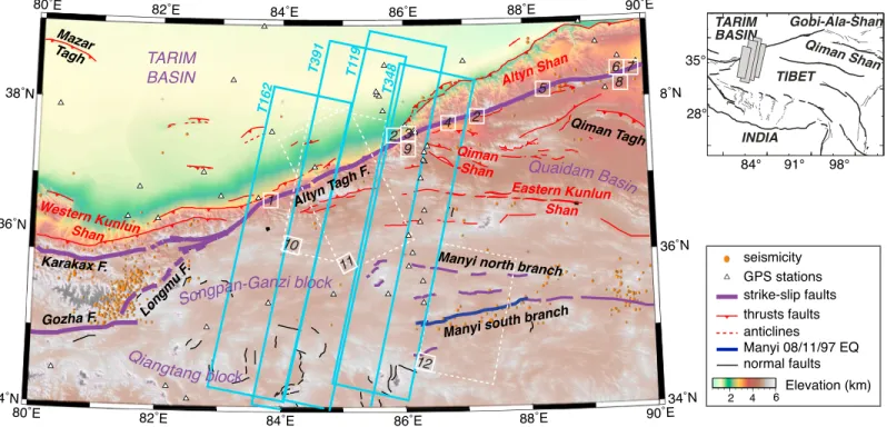
Figure 1. Seismotectonic setting of the Altyn Tagh Fault system superimposed on Digital Elevation Model of the Shuttle Radar Topography Mission
(Farr & Kobrick, 2000). Fault traces are modified from Van Der Woerd et al. (2002) and Replumaz and Tapponnier (2003). Orange dots show the seismicity from 1992 to 2014 from USGS. Black triangles are GPS stations from the Observation Network of China (Wang et al., 2017) and from the GPS transect of He et al. (2013). Surface traces of four overlapping Envisat descending tracks 162, 391, 119, and 348 used in this study are in cyan. Previous interseismic slip rate investigations include Quaternary time scale measurements from offset risers and glacial features from (1) Peltzer et al. (1989) (∼20–30 mm/yr), (2) Mériaux et al. (2004) (27 ± 7mm/yr), (3) Cowgill (2007) (9.4±2.3), (4) Gold et al. (2009) (∼7–17 mm/yr), (5) Cowgill et al. (2009) (11.5 ± 2.5mm/yr), and (6) Mériaux et al. (2012) (14 ± 1mm/yr); paleoseismic measurements from (7) Washburn et al. (2001) (∼10–20 mm/yr); GPS transects measurements from (8) Wallace et al. (2004) (9 ± 4mm/yr) and (9) He et al. (2013) (9 ± 4mm/yr); and interferometric synthetic aperture radar studies across the Altyn Tagh Fault from (10) Elliott et al. (2008) (11 ± 10mm/yr) and from (11) Zhu et al. (2016) (8 ± 0.7mm/yr), as well as across the MF, which broke during the 1997M7.6 earthquake (blue line), from (12) Bell et al. (2011) (3 ± 2mm/yr).
a minor role in accommodating the continental shortening (e.g., Bendick et al., 2000; Wallace et al., 2004; Wright et al., 2004; Zhang et al., 2004). Yet another class of models describes the presence of a low-viscosity layer (< 1018Pa s) within the crust due to increased radiogenic heat production in thickened crust (Clark &
Royden, 2000; Cook & Royden, 2008; Royden et al., 1997). This low-viscosity layer would result in significant mass transport in response to pressure gradient. This “channel” would flow more easily than either the over-lying brittle upper crust or the underover-lying mantle lithosphere, transporting material and contributing to the growth of the flat topography. Low-viscosity layers, potentially transient, have been evidenced by interfer-ometric synthetic aperture radar (InSAR) measurements on some parts of the Tibetan Plateau from far-field postseismic displacements (Huang et al., 2014; Ryder et al., 2007, 2011; Wen et al., 2012) or by lake surface and level changes (Doin et al., 2015). However, they suffer from trade-offs between the viscosity and the depth of the deformation and from our poor knowledge of the steady state rheology of the crust at longer time scales (e.g., DeVries & Meade, 2016; Leloup et al., 1999).
InSAR data provide unique information to characterize the present-day deformation of Tibet, in particular in western and central Tibet, where GPS data are critically sparse (e.g., Liang et al., 2013; Wang et al., 2017). Major faults such as the ATF, the KF, and the KJFZ fault systems are therefore poorly covered by GPS network in the near field (Figure 1). InSAR provides continuous maps of deformation throughout broad regions and therefore precisely constrains the fault’s interseismic loading and its lateral variations. However, because of many data processing challenges, only a few studies attempted to measure interseismic deformation in the western part of Tibet (e.g., Bell et al., 2011; Elliott et al., 2008; Garthwaite et al., 2013; Jolivet et al., 2008; Wang & Wright, 2012; Wright et al., 2004; Zhu et al., 2016).
With its remarkable morphology and 4 km of relief, the ATF is the main active structure along the northern boundary of the Tibetan Plateau (Cheng et al., 2016; Jolivet et al., 2001; Matte et al., 1996; Molnar & Tapponnier, 1975; Peltzer et al., 1989; Yin & Harrison, 2000) (Figure 1). If stable for a long period of time, a high slip rate on the ATF would accommodate a large part of the India-Asia convergence (Avouac & Tapponnier, 1993; Mériaux et al., 2004; Mériaux et al., 2004, 2005, 2012; Peltzer & Saucier, 1996; Peltzer et al., 1989; Washburn et al., 2001; Xu et al., 2005). It would only leave negligible convergence within Tibet and transfer most of the convergence to the thrust and fold systems in the Qaidam basin and the Qilian Shan (Jolivet et al., 2008; Lasserre et al., 2007; Tapponnier et al., 2001). Conversely, a low rate on the ATF would require some deformation distributed through the plateau and possibly larger slip rates on some other secondary faults (Bendick et al., 2000; Cowgill, 2007, 2009; Gold et al., 2009; He et al., 2013; Wallace et al., 2004; Zhang et al., 2004; Zhu et al., 2016) (Figure 1). In this paper, we focus on the northwestern part of the Tibetan Plateau between longitudes 83∘ and 87∘ (Figure 1). We processed four 100 km wide Envisat descending tracks from the Tarim basin, north of the ATF, to the central part of Tibet covering the western termination of the Manyi Fault (MF), which ruptured during the 1997 M ∼8 Manyi earthquake (Funning et al., 2007; Peltzer et al., 1999; Ryder et al., 2007; Wang et al., 2007). For most of this section (83∘ –86∘) the ATF is relatively simple with a single branch at the foot of the large topographic step between Tibet and the Tarim basin (Figure 1). East of 86∘, the ATF enters zones of higher topography between the Altyn Shan to the north and the Qiman Shan to the south. Both these ranges are compressional structures with an active thrust along the northern front of the Altyn Shan and smaller thrust faults branching off to the south. West of 83∘, the ATF enters the western Kunlun range and branches into a thrust system at its northern front and the left-lateral Longmu-Gozha Fault to the south (Figure 1). Quaternary deformation of sediments along the southern edge of the Tarim basin confirms the convergence between the Tarim and Tibetan blocks (Matte et al., 1996; Jiang et al., 2013). The thrust-system foreland extends to the Mazar Tagh range along a décollement rooting on the ATF that reaches up to the middle part of the Tarim basin over a width of about 500 km (Coudroy et al., 2009; Guilbaud et al., 2017; Wittlinger et al., 2004) (Figure 1). Recent earthquakes, such as the 2015 Mw6.4 Pishan earthquake that broke a blind thrust north of the west-ern Kunlun Shan, are evidence of the strain accumulation along these deep thrust systems (Lu et al., 2016; Sun et al., 2016), which now need to be considered in kinematic models.
In this study, we develop methodologies to address InSAR processing challenges and separate the tectonic signal from surface and atmospheric noise processes. We produce a line-of-sight (LOS) velocity map covering a broad region in the northwestern part of the Tibetan Plateau, shedding light on the kinematics of the western part of the ATF and associated faults. We then provide quantitative estimates of the loading rate and the range of geometries consistent with surface velocities observed by InSAR and GPS using a Bayesian framework and assuming conservation of motion across the fault network.
2. InSAR Processing
2.1. State of the Art
InSAR is a powerful tool to map precisely and over large areas surface displacements (e.g., Bürgmann et al., 2000; Hooper et al., 2012). This technique has been widely employed in earthquake and fault studies (e.g., Jolivet et al., 2013; Pathier et al., 2003; Rousset et al., 2016; Sudhaus & Jónsson, 2011; Wimpenny et al., 2017), volcanic dike intrusions (e.g., Cervelli et al., 2002; Grandin et al., 2009; Manconi & Casu, 2012; Pedersen & Sigmundsson, 2006), landslide monitoring (e.g., Fruneau et al., 1996; Hilley et al., 2004; Schlögel et al., 2015; Strozzi et al., 2013; Wasowski & Bovenga, 2014), urban subsidence (e.g., Amelung et al., 1999; Bawden et al., 2001; Fruneau & Sarti, 2000; López-Quiroz et al., 2009), permafrost freeze-thaw cycles (e.g., Chang & Hanssen, 2015; Daout et al., 2017; Liu et al., 2010; Short et al., 2011), or water vapor mapping (e.g., Hanssen et al., 1999; Wadge et al., 2002). However, for small deformation signals in high mountainous areas, such as interseismic deformation, the approach suffers from major limitations due to high topographic gradients and unsuitable valley flank orientations relative to the synthetic aperture radar (SAR) view angle, snow cover, or atmospheric delays. Within the Tibetan Plateau, Taylor and Peltzer (2006) measured by InSAR the surface velocity field associated with the Gyaring Co fault and quantified a localized surface displacement along conjugated faults. They first pointed out the difficulties associated with the deformation induced by freeze and thaw cycles and the atmospheric delay changes across the topographic steps (Figure S1 in the supporting information). Elliott et al. (2008), Jolivet et al. (2008), Wang and Wright (2012), Wright et al. (2004) and Zhu et al. (2016) quantified the interseismic surface displacements associated to the ATF (Figure 1) but faced the numerous ambiguities
and trade-offs between the tectonic deformation and topography, phase delays associated with stratified troposphere, or orbital ramps. To deal with these problems, Elliott et al. (2008) or Wang and Wright (2012) inverted InSAR maps, solving simultaneously for parameters describing the nontectonic processes and the slip rates on faults. This resulted in large uncertainties on the velocity gradients across fault due to the strong trade-off between the different parameters (Figure S1b). Moreover, due to the radar phase coherence loss along the sand dunes in the south of the Tarim basin and in some sedimentary basins within the plateau, these previous studies are restricted to using data in the near field of the ATF, although the far-field signal is important to accurately constrain fault slip rate. Bell et al. (2011) measured 3 ± 2 mm/yr of interseismic motion across the MF prior to the 1997 earthquake (Figure 1), but the high level of noise reveals the impor-tance of taking into account surface processes affecting the coherence of the interferometric phase. Wang and Wright (2012) and Garthwaite et al. (2013) describe the first attempts to process long radar tracks across the Tibetan Plateau. There again, coherence loss and the contribution of atmospheric signal limited the pos-sibility to resolve tectonic rates without ambiguities in all areas. For example, Wang and Wright (2012) did not unwrap the interferometric phase across the ATF and studied separately the northern and the southern parts of the fault.
2.2. Data Set and Formation of Wrapped Interferograms
We processed the complete Envisat descending archive along four 500 km long and 100 km wide Envisat over-lapping tracks (162, 391, 119, and 348) between 2003 and 2011 (Figure 1). To obtain displacement time series in this natural environment and limit the effects of phase decorrelation, we constructed 484 small baseline differential interferograms with the New Small Baselines Subset chain (NSBAS) (Doin et al., 2011, 2015) based on the ROI_PAC software (Rosen et al., 2004).
Single Look Complex images are computed from the raw radar data in a common mean Doppler geome-try. Single Look Complex images are resampled to a single master image geometry, and a slope-dependent range spectral filter is applied to increase the coherence in interferograms with long perpendicular baselines (Guillaso et al., 2006). A network of SAR image pair combinations is defined using spatial and temporal baseline constraints ensuring redundancy (Figure S2). Interferograms are formed with two range looks and 10 azimuth looks (∼ 40 × 40 m2) to obtain coarser differential interferograms, and a linear ramp in range is removed to
account for orbital errors and clock drift (Fattahi & Amelung, 2014; Lauknes et al., 2011; Zhang et al., 2014). Removing such linear ramp may not necessarily remove orbital errors as long wavelength tectonic signals can trade off against the ramp (Biggs et al., 2007). Therefore, a second ramp will be removed later to account for this during the modeling. InSAR-derived deformation maps are thus exempt of any uniform tilt in range. Finally, the signal-over-noise ratio (SNR) of the wrapped differential interferograms is improved by correct-ing local digital elevation model (DEM) errors exploitcorrect-ing the phase versus perpendicular baseline relationship (Ducret et al., 2014). The correction reduces up to 20% the wrapped phase variance on interferograms, limiting apparent phase decorrelation in areas of high relief (Figures S3 and S4).
2.3. Atmospheric Delays Correction
The atmospheric radar phase delay is divided into a turbulent component and stratified component, which correlates with the topography(Hanssen, 2001). The spatial phase patterns produced by the turbulent atmo-sphere being random both in space and time can be attenuated by smoothing the time series. In contrast, the stratified tropospheric phase delay shows smooth variations in time and is dominated by a seasonal term (Cavalié et al., 2007; Doin et al., 2009; Fattahi & Amelung, 2015) with an amplitude depending on variation of temperature, pressure, and relative humidity. The stratified tropospheric delay in interferograms can reach few centimeters per kilometer of elevation and often overprints any small deformation. Correcting this signal is thus one of the most important processing steps, first, to prevent unwrapping errors in mountainous areas and, second, to reach an accuracy of a few millimeters per year on ground velocities.
Two classes of methods have been developed to correct for the tropospheric phase delay. The first one empir-ically exploits the correlation between the interferometric phase and the elevation (Béjar-Pizarro et al., 2013; Bekaert et al., 2015; Cavalié et al., 2008; Doin et al., 2015; Lin et al., 2010; Shirzaei & Burgmann, 2012; Tymo-fyeyeva & Fialko, 2015) (Figure S5). These approaches are effective at reducing the interferometric phase variance but may remove some displacement-related signal when deformation correlates with topography. This is a critical issue for the Tibetan margin because of the 4 km topographic step between the Tarim basin and the high plateau, colocated with the expected gradient of surface displacement associated with slip on the ATF (Figure S1b). We show, in a synthetic test, that the simulated signal produced by interseismic strain
along a strike-slip fault aligned with the ATF can be partly or entirely removed by applying a correction based on empirical phase-topography correlation, depending on the parametrization used (supporting information Figure S6).
The second class of atmospheric correction method consists in estimating the phase delay using auxiliary data such as GPS delay measurements (Li et al., 2006; Webley et al., 2002; Williams et al., 1998), satellite mul-tispectral imagery (Li et al., 2012), meteorological data (Delacourt et al., 1998), or global atmospheric models (Doin et al., 2009; Jolivet et al., 2011, 2014). In this study, we estimate the phase delay due to the stratified tro-posphere using the global atmospheric reanalysis model ERA-Interim (ERA-I) from the European Centre for Medium-Range Weather Forecasts (Dee et al., 2011). ERA-I provides estimates of temperature, water vapor partial pressure, and geopotential height every 6 h at 37 pressure levels on a 0.7∘ grid from 1989 to present (Dee et al., 2011). Integrated path delays at acquisition times, computed from both hydrostatic and wet delay contributions, are derived at ERA-I points encompassing a SAR scene, using vertical profiles of these variables. The delay is then mapped on the radar scene using a DEM. When several ERA-I points are used, bilinear inter-polation in the horizontal direction is performed on the vertical profiles. However, in the presence of steep topography, interpolating model parameters between grid nodes at largely different elevations can produce artifacts in the phase delay maps because the weather model must be extrapolated below the surface of the Earth. To avoid this problem, we compute the atmospheric phase delay maps using ERA-I parameter values from the node with the lowest elevation within the radar scene (Doin et al., 2009) (Figure S7). This correc-tion is validated by comparison with empirical estimacorrec-tions (supporting informacorrec-tion). In the following seccorrec-tion we assess the possible error on the atmospheric phase delay correction. Our objective is to provide an error bound on the LOS surface velocity due to the atmosphere.
2.4. Uncertainties on Velocity Maps Due To Stratified Atmospheric Delays
Velocity maps are known to be polluted by aliasing of oddly sampled time-varying atmospheric signals (Doin et al., 2009). To analyze the impact of the atmospheric correction on the expected velocity map, we com-pare the 1 day resolution time series of the phase delays predicted by ERA-I at two points (two ERA-I nodes in Figure S2), in the overlapping area of the two tracks 119 and 391. One is located in the Tarim basin (38.25∘N, 85.5∘E), at the lowest elevation (altitude of 1.4 km), and the other one is in the Tibetan Plateau (36.75∘N, 85.2∘E), closest to the ATF, at an altitude of 4.5 km (Figures 2 and S7). We simulate fictitious velocity maps cal-culated solely with the ERA-I delay prediction over the topography of the Tibetan Plateau at SAR acquisition time (Figure S9). We use 7 day moving windows to compute an average time series S7dand a standard
devi-ation𝜎k. The justification of this 7 day moving average is based on the comparison with empirical estimates
(Figure S8). It is large enough to bracket extreme dry or wet events but small enough to keep the temporally correlated variability.
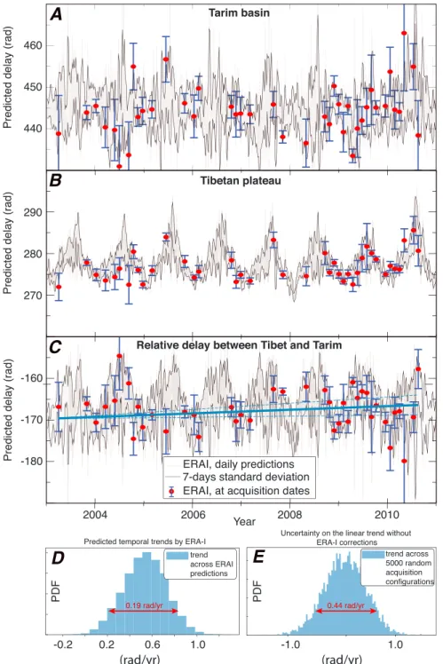
We observe within the Tarim basin (Figure 2a) a strong daily variability of ∼ 6.5 rad (=∼ 29 mm) and a small seasonality of ∼ 2.5 rad (=∼ 5.5 mm) in amplitude, while within the Tibetan Plateau (Figure 2b), the ERA-I model predicts a regular seasonal signal of ∼ 8 rad (= ∼ 17 mm) in amplitude and a higher daily variabil-ity in summer (∼ 5 rad = ∼ 22 mm) than in winter (∼ 1.5 rad = ∼ 7 mm). The delay differences (Figure 2c) show a slight seasonal signal of ∼ 6 rad (=∼ 13.5 mm) of amplitude and a strong daily variability of 5.5 rad (=∼ 24.5 mm). The delays at acquisition dates (shown with red circles in Figure 2) are sometimes clearly outside the𝜎kenvelope.
Because of the few control points of air moisture in this remote area, ERA-I may not well predict the very quick variations in delay that are associated to abrupt changes in humidity and, to a lesser extent, in temperature. We thus use the 7 day standard variations,𝜎k=i, centered on the date i, as a proxy for errors in ERA-I predic-tion. Furthermore, some computed delays that appear as outliers in the time series may be more prone to an erroneous prediction by ERA-I. We therefore define a proxy,𝜎p,i, for the uncertainty on Sifor each acquisition date i, such as
𝜎p,i=𝜎k=i, if |Si− S7d| < 𝜎k=i, (1)
𝜎p,i=|Si− S7d|, otherwise. (2)
In short, if the daily acquisition, Si, is close to the sliding window average model, S7d, and within the envelope, 𝜎k, then the error,𝜎p,i, is equal to the standard deviation at the date i,𝜎k=i. Otherwise, if the daily acquisition, Si, is an outlier (i.e.,|Si − S7d| > 𝜎k=i) then the error,𝜎p,i, is equal to its absolute distance to the average.
Figure 2. Predicted phase delay time series from ERA-Interim atmospheric model,Sk=i(red circles), plotted as a function of time superimposed to the daily model (gray lines) and the 7 day sliding windows standard deviation𝜎k(black lines).
(a) Relative delay in between the satellite and the Tarim basin (38.25∘N, 85.5∘E) located at 1,400 m height. (b) Relative delay in between the satellite and the Tibetan Plateau (36.75∘N, 85.2∘E) located at 4,500 m height. (c) Relative delay in between the Tibetan Plateau and the Tarim basin (two ERA-I nodes in Figure S5) with associated error bar proxies,𝜎p,i. (d) Predicted temporal trend,Δv, and uncertainties,𝜎ERA-I
Δv across the Altyn Tagh Fault due to the atmosphere from ERA-I
models weighted by the defined error proxy. (e) Computed uncertainty,𝜎Δv, between Tibet and Tarim, if no atmospheric corrections were applied.
The error bar proxies on the absolute and relative delays are drawn in Figure 2. Note that a few acquisitions have a𝜎p,ivalue clearly larger than others. We assume that their ERA-I corrections are less reliable than for other acquisitions. Note also that the average𝜎k(∼ 2.1 rad = ∼ 9.5 mm) is lower than the absolute S variability by a factor of 3 (∼ 5.9 rad). Empirically derived phase-elevation relationships (Figure S8) show that 𝜎p,ierror proxy corresponds to an upper bound on the 1𝜎 error on ERA-I-derived delays. This proxy is thus a conserva-tive estimate of errors on ERA-I that allows to include all empirical measurements. In the following time series analysis, these ERA-I-derived uncertainties are used to weight each acquisition and thus better constrain the linear trend across the ATF due to the aliasing and variability of the tropospheric seasonal signal.
From this analysis, we can draw the following conclusions regarding the uncertainty on the relative velocity across the ATF. First, if the data were not corrected from stratified atmospheric delays, we would expect a tem-poral bias, Δv, corresponding to the temtem-poral trend in rad/yr across the Sivalues. To quantify statistically this
potential bias, if no atmospheric corrections were applied (Figure 2e), we randomly sample the daily model Si 5,000 times (keeping the spread of the actual Envisat sampling) and compute the temporal linear trend at each iteration. The predictions show a gaussian distribution centered on 0 with an uncertainty,𝜎Δv, of 0.44 rad/yr = 1.96 mm/yr. Second, we can infer that the sign and amplitude of this trend will strongly depend on the data sampling within the seasonal cycle (relatively random). We finally compute the velocity gradient due to the atmosphere, Δv, from the ERA-I predictions at acquisition dates (blue line in Figures 2c, 2d, and S10) and derived its uncertainty,𝜎ERA-I
Δv (blue dashed lines in Figures 2c, 2d, and S10) by propagating the defined error
proxy at each acquisition date into an error on the linear trend. To summarize, the ERA-I corrections impact the relative velocity observed across the ATF by −1.85 to 2.45 mm/yr across the ∼3 km of topography, with a conservative uncertainty on the velocity of 0.8–1.3 mm/yr on the four studied tracks (Figure S10). The ERA-I correction thus reduces the uncertainty on the velocity across the Tibet border by a factor of 2.
2.5. Unwrapping Procedure of the Interferometric Phase
South of the ATF, the plateau is shaped by narrow, E-W mountain ranges reaching elevations of ∼6,000 m, bounding quaternary sedimentary basins at an elevation of ∼4,400 m. These sedimentary basins contain soils with permanent ice, called permafrost, with an active layer affected by the seasonal freeze-thaw cycle, result-ing in the upheaval and subsidence of the soil and other cryoturbations processes that degrade the coherence of the radar signal. As described in Daout et al. (2017) and in the supporting information, we implement a specific method to unwrap the interferometric phase delay, that consists in removing a spatial template of deformation to help the unwrapping across the sedimentary basins where we observe strong phase gra-dients. This approach is standard in InSAR processing and has already been applied for land subsidence (e.g., López-Quiroz et al., 2009; Strozzi & Wegmuller, 1999) or volcanic (e.g., Pinel et al., 2008; Yun et al., 2007) studies in presence of complex and large surface displacements. Here we extract the template from a prin-cipal component analysis decomposition of a series of well unwrapped interferograms (Figure S11). We also apply different phase filters, which are a weighted average of the interferometric phase in sliding windows, to help the unwrapping across the alluvial fans and sand dunes, north of the ATF (Figure S12) (Grandin et al., 2012; Pinel-Puyssegur et al., 2012). Doing so, we successfully unwrap interferograms from north to south. Finally, checking misclosure in the interferometric network allows to identify remaining unwrapping errors and correct them manually (López-Quiroz et al., 2009).
2.6. Residual Orbit Errors and Time Series Analysis
Before constructing the time series of the LOS displacement observed by InSAR, it is important to define a reference frame (Figure S13). The observation of the interferograms of northwestern Tibet (Daout et al., 2017) showed that the observed phase change contains the tectonic signal along active faults, the seasonal signal associated with the freeze-thaw cycle of the permafrost active layer in basins, and overall ramps due to resid-ual orbit clock drift errors. Here we refer all interferograms with respect to the bedrock in the area between the ATF and the western termination of the MF (Figure 1). The bedrock reference frame is defined by masking the sedimentary basins where a strong (larger than>2.5 mm) seasonal signal is observed (Daout et al., 2017). The referencing is done as follows. For each interferogram, one azimuthal ramp is adjusted to the bedrock pixels. The ramp is generally quadratic in both azimuth and range for long interferograms, or linear for short interferograms with missing frames. The ramps are then optimized in the network of interferograms to ensure internal consistency. Finally, the optimized, reconstructed ramps are removed from each interferogram (supporting information section S4.2).
Figure 3. Line-of-sight (LOS) velocity map of the four tracks 162, 391, 119, and 348 displayed for an average incidence angle of 23.5∘and referred to the area located between the ATF and the Jinsha suture. Fault traces and GPS stations as in Figure 1. Surface trace of the suture zone is from Taylor and Yin (2009). Black arrows point out gradients of deformation. Positive motion is toward the satellite. Blue (motion away from the satellite) and red (motion toward the satellite) ellipse is a schematic representation of the postseismic of the Manyi Earthquake according to Ryder et al. (2007). AA′, BB′, CC′, and DD′= four profiles across observed velocity gradient described in Figures 4 and 8.
Time series of LOS displacement are then constructed using the NSBAS method (Doin et al., 2015) with a linear regularization function of the form
𝜙i= V × ti+𝛼Bi⟂. (3)
where𝜙iis the pixel phase change between time t and the first epoch, V, the best estimate of the pixel LOS velocity,𝛼, an estimate of the residual DEM error, and Bi
⟂is the perpendicular baseline of acquisition i. Maps of
DEM error coefficients display typical oblique striations and are consistent between overlapping areas (Figure S14) at short-wavelength (with some residual long-wavelength ramps between adjacent tracks). Note that for Envisat data the velocity estimation does not trade off with the DEM error correction as the perpendicular baseline does not drift with time (Figure S2). Each equation set (3) is weighted by the inverse of the ERA-I correction uncertainty,𝜎p,i, obtained for each image, i (section 2.4).
The same processing is applied to all four tracks. To combine all velocity maps in a single map (Figure 3), we started by referencing the velocity field of the central track (119) to the bedrock pixels located south of the ATF and north of the Jinsha suture with a linear adjustment in azimuth. Then, the LOS velocity maps of the three other tracks were adjusted with respect to one another by adding the ramp in azimuth that minimizes the difference in the overlapping areas between adjacent tracks (Figure S15). Because the surface displacements
Figure 4. Line-of-sight (LOS) velocity of two stack profiles across active structures in NW Tibet. See Figure 3 for location. AA′= Altyn Tagh Fault (ATF)-perpendicular profile encompassing the four tracks. Color scale depending on the
along-ATF distance (blue = west, yellow = east). Arrows point to five velocity gradients associated with Jinsha suture, Qiman-Kunlun thrusts, ATF, Altyn Shan thrusts, and the Cherchen Fault. BB′= profile perpendicular to Qiman Shan and
along the azimuth of the track, extending from Tarim basin to southern branch of Manyi Fault. Green crosses = GPS velocities projected along the B-B′profile, that is, oblique to the ATF strike (see section 4.1 for GPS data processing).
Arrows point to six velocity gradients associated with southern and northern branches of the Manyi Fault, Kunlun thrusts, Qiman Shan thrusts, ATF, and Altyn Shan thrusts.
are expected to be mostly horizontal along the strike-slip system, we normalize velocity maps to a constant incidence angle of 23.5∘. This is done by scaling the LOS velocity of each track by sin(23.5∘)/sin(𝜃), where 𝜃 is the local incidence angle. Note that this harmonization is only used for map visualization of section 3 and not for the following modeling part in section 4.2. The discrepancy of the normalized LOS velocities in overlapping areas between adjacent tracks (e.g., Wen et al., 2012) is of 0.4–0.8 mm/yr (Figure S15c).
3. LOS Velocity Field in Northwestern Tibet
The final LOS surface velocity map shows for the first time an almost continuous view of the surface displace-ment field over a broad area (300 km × 500 km) in NW Tibet that remains largely uncovered by GPS data (Figure 3). Areas where large seasonal movements associated with the permafrost active layer are observed have been masked for clarity. The first-order features of the velocity field are the steep gradient across the ATF showing the overall eastward movement of Tibet (red-yellow tones, toward the satellite) with respect to the Tarim block (blue tones, away from the satellite), and a distributed gradient along an east-west trend at the latitude of the Jinsha suture (Figures 3 and 4). In addition, a zone of relatively low velocity is observed in the eastern part of the covered area between the eastern Kunlun Shan and the northern branch of the MF (Figure 4). These features are observed in the decadal linear trends of the InSAR time series and most likely represent tectonic surface displacements associated with the active faults in NW Tibet. At a more detailed level, deformation is also visible north of the ATF, along the southern rim of the Tarim basin (Figure 5).
3.1. Transpressional Deformation Along the Northern Edge of Tibet
The LOS surface velocity difference of ∼3–4 mm/yr observed between the northern Tibet bedrock and the southern Tarim is consistent along the 300 km wide section covered by the four radar tracks used in this study.
Figure 5. (a) Zoom on Figure 3 in the foreland of the Tibetan Plateau south of the Tarim basin. (b) Topographic (dark lines) and line-of-sight (LOS) velocities (purple = track 348, orange = track 119, red = track 391, and blue = track 162) profiles perpendicular to the Altyn Tagh Fault (ATF). The white lines in (a) indicate the location of the nine 160 km long and 20 km large profiles. (c) Zoom around a north dipping thrust fault cutting an alluvial fan in the Tarim basin (black rectangular box annotated (c) in panel (a) from an ASTER multiband image. (d) LOS velocity profile from track 162 (blue dots) within the Tarim basin across the north dipping and south dipping thrusts (black rectangular box annotated (d) in panel (b) with interpreted fault structures. Black and white arrows point out observed velocity gradients in the Tarim basin.
The surface velocity gradient occurs within a 30 km wide zone along the active trace of the ATF (Figures 3 and 4). We interpret this signal primarily as the elastic displacement rate associated with the left-lateral movement on the deep part of the ATF.
Around longitude ∼ 86∘, the data indicate velocity changes associated with the slight change of azimuth of the ATF and its connection with the Qiman Shan and eastern Kunlun Shan thrusts, 70 km south of the ATF (Profile BB′in Figure 4). Approximately 1 mm/yr of velocity change is observed, a gradient consistent
with that produced by interseismic strain across a north dipping thrust, south of the Qiman Shan. Similarly, the strong velocity gradient with opposite sign observed 40 km north of the ATF could be associated with the south dipping Altyn Shan thrusts (Figures 4b and 5a). This displacement exhibits a linear temporal evolution in the InSAR time series, indicating that a tectonic origin is more likely than a hydrological process. In addition, Google Earth images show that the recent deposits and drainage at the foot of the Altyn Ranges are disrupted by active thrusts.
The InSAR data also show a sharp step in velocity along a linear structure at the base of the alluvial fans along the foreland of Tibet (Figures 3, 4 (Profile AA′), and 5), referred to as the Cherchen Fault in
previ-ous studies (Yin & Harrison, 2000). We ruled out any unwrapping errors or hydrological deformation in this area by checking for the absence of misfit misclosure and seasonal behavior in the time series analysis.
Assuming a tectonic origin of the deformation, the velocity gradient can be related to either left-lateral shear or uplift above a south dipping thrust. The velocity profiles across this structure indicate a LOS veloc-ity decrease to the north by 0.2–0.6 mm/yr (Figure 5). Furthermore, the profile in Figure 5d shows a slight gradient in the opposite sign 20–25 km south of the linear structure. These changes in velocity are aligned and probably associated with thrust faults mapped along the southern rim of the Tarim basin from the anal-ysis of seismic profiles (Laborde, 2017). The structure is a continuous, south dipping thrust fault affecting basement rocks under the Cenozoic sediments in southern Tarim. The more subdued signal observed south of the main structure (centered at 37.4∘N, 84.4∘E) corresponds to a north dipping, back-thrust fault that reaches the surface across the Moleqie River fan, clearly visible in the Advanced Spaceborne Thermal Emis-sion and Reflection Radiometer (ASTER) visible and near-infrared enhanced image shown in Figure 5c. The image highlights the older terraces of the fan uplifted with respect to the active channels (Laborde, 2017). Together, the south dipping and north dipping faults form the Tanan pop-up structure lifting up a 20–25 km wide portion of crust. We interpret both changes in LOS velocity in this area to be the result of the verti-cal movement associated with the thrust faults currently locked in the upper part of the crust (Figure 5d). These findings indicate that the northern edge of Tibet along the studied section is a transpressional bound-ary with left-lateral motion parallel to the ATF and convergence perpendicular to it. In continuity but with less intensity than the convergence observed north of the Kunlun ranges (Guilbaud et al., 2017; Lu et al., 2016; Matte et al., 1996; Sun et al., 2016), the shortening is accommodated north of the ATF in the thrust system that formed along the distal part of the foreland alluvial fans. In the fault interpretation outlined in Figure 5d, the transfer of the convergence component of movement is achieved through a flat décollement up to the northernmost thrust.
3.2. Apparent Shear Zone Along Jinsha Suture
The second outstanding feature of the LOS surface velocity field is the broad east-west oriented shear zone that approximately follows the late Triassic Jinsha suture between the Qiangtang terrane to the south and the Songpan-Ganzi terrane to the north (e.g., Tapponnier et al., 2001; Yin & Harrison, 2000) (Figure 3). The velocity map shows a distributed gradient of deformation centered on an axis near latitude ∼ 92∘N , extending along the Jinsha suture from the termination of the MF, which broke in 1997, in the east, to the Gozha Fault in the west (Figure 3). Active fault mapping from Landsat optical images does not show any continuous fault surface trace along the suture (Tapponnier & Molnar, 1977), but geological maps and high-resolution images avail-able in Google Earth clearly reveal the fabric of the crust in the suture zone, with WNW-ESE oriented, steeply dipping strata of a thick series of marine sediments referred to as the Songpan-Ganzi flysch complex in central Tibet (e.g., Yin & Harrison, 2000). The propagation of a clear-cut strike slip fault may be difficult in such a highly anisotropic terrane, more prone to distributed deformation involving discontinuous fault segments interact-ing with the structure of the folded units. The LOS velocity change across the Jinsha suture is ∼3-4 mm/yr with the southern side moving toward the satellite compared to the northern side (Figure 4). This signal does not have the characteristics of a velocity field caused by a thrust fault as the uplift would be concentrated at the tip of the creeping ramp and would die off away from it. We therefore interpret the signal as a broad shear zone accommodating left-lateral movements between the Qiangtang and the Songpan-Ganzi blocks. The signal could also be associated with a transient process following the 1997 Manyi earthquake (Figure 4), although no time dependence has been detected in the data.
The data also reveal a steep LOS velocity change of ∼1–2 mm/yr across the western end of the northern branch of the MF (Figure 3 and profile BB′in Figure 4), which may extend farther west of our study area along
the northern boundary of the large permafrost basin (masked area in Figure 3, blue pixels in Figure S11). GPS data do not reveal any clear shortening across this potential structure, which may be interpreted as a secondary strike-slip fault of the MF system.
Finally, we observe a negative LOS velocity change of ∼1–2 mm/yr, 0–50 km south of the ATF (Profile BB′
in Figure 4), only visible in the eastern part of the study area (Figure 3). Here GPS data indicate 2–3 mm/yr of shortening velocity, which may also suggest vertical movements associated with contraction in the north dipping thrusts of the eastern Kunlun and Qiman ranges (Figure 3).
4. Kinematic Modeling
4.1. Comparison With GPS Data
We first compare our surface velocity map with GPS data provided by He et al. (2013), which includes 17 cam-paign stations measured two to three times between 2009 and 2011, and with the regional data set provided
Figure 6. GPS velocities from Wang et al. (2017) and from He et al. (2013) referred with respect to the Tarim block and superimposed to the amplitude of the seasonal deformation due to the freeze and thaw cycles of the permafrost active layer derived in Daout et al. (2017). We use stations I033, I063, I064, XJTZ, and I065, located in the Tarim basin and far from any faults, to invert for the parameters of the Euler pole between the Tibetan and the Tarim blocks, which lies at latitude 45∘49′and longitude−62∘7′with a clockwise angular velocity of 0.282 Ma−1. Fault traces are as in Figure 1.
AA′= 200 km large and 300 km long profiles across the central segment of the ATF used in the model.
by Wang et al. (2017), which includes 23 continuous and campaign stations measured two to three times in our study area acquired between 1999 and 2014. In Figure 6, we superimpose the station locations on the amplitude of the ground seasonal deformation associated with the freeze-thaw cycle of the permafrost active layer (Daout et al., 2017). We observe that at least AT05, AT10, AT11, J343, and J344 stations are located within sedimentary basins that undergo strong seasonal deformation. The velocity estimated after two or three measurement campaigns must therefore be interpreted with caution at these stations.
In order to compare the GPS field of Wang et al. (2017) with the GPS solution of He et al. (2013), we rotate the International Terrestrial Reference Frame (ITRF) solution of Wang et al. (2017) with respect to the Tarim block, north of the ATF, and display the ATF-perpendicular and the ATF-parallel GPS velocity components for the two networks in Tables S1 and S2. On the eastern side of our study area, GPS stations I035, XJRQ, I034, I400, and I398 of Wang et al. (2017) (Table S2) clearly show the shortening component north of the Altyn Shan. GPS stations XJQM, I036, and I405 indicate a shortening and shearing relative to stations J333 and J343 of 2–5 mm/yr and ∼8 mm/yr, respectively. However, as discussed above, we consider the velocity of these two stations (J343 and J344) as unreliable due to seasonal deformation of the permafrost active layer (Figure 6). In comparison, the velocity gradient from He et al. (2013) (Table S1) shows a left-lateral far-field motion of ∼8–10 mm/yr centered on the ATF and indicates no clear convergence between far-field stations in Tarim and Tibet (Figure 6). As seen in our velocity map, GPS stations AT14, AT15, AT01, AT02, AT03, AT03A, and AT04 seem to indicate a left-lateral or a thrust movement linked to the activity of the Qiman Shan.
Figure 7. Inversion model and results for the profile perpendicular to the Altyn Tagh Fault (ATF) defined in Figure 6. (a) (top) Minimum, maximum, and average topography along the swath profile (back and gray lines), posterior models in agreement with the data (blue lines), and average posterior geometry
(thick black lines) with associated slip rates. (middle) LOS velocities (cyan, blue, red, and orange points) along the swath profile (Figure 6). (bottom)
Fault-perpendicular (green triangle and inverted triangle markers) and fault-parallel (blue triangle and inverted triangle markers) GPS velocities. Average model obtained and corresponding to fault-parallel, fault-perpendicular, and vertical velocities in blue, green, and orange lines, respectively, along profile. (b) Posterior marginal Probability Density Functions (PDFs) using GPS data only or InSAR data only (black and red unfilled histograms, respectively) or GPS+InSAR data (blue filled histograms), showing the gain of information from InSAR data. The boundaries of the histograms correspond to the uniform prior distributions.
4.2. Two-Dimensional Profile Across the ATF
We use the Bayesian inversion tool developed in Daout, Barbot, et al. (2016) to constrain the tectonic loading rate on the ATF system. We explore various fault geometries in agreement with the observed displacements along a 200 km wide and 300 km long profile covering the two GPS networks and four InSAR velocity maps (profile AA′in Figure 6). The model includes four dislocations embedded in an elastic half-space (Okada,
1985) (Figure 7). First, a deep-seated dislocation, with a tip depth, LDShear, below the ATF accommodates both
far-field shortening (Vshort) and fault-parallel left-lateral horizontal movement (SSATF) between Tarim and Tibet.
Connecting to the tip of this dislocation, we define two other segments: a first segment extends the creep on the ATF upward by a distance, HATF, and a second segment is a flat structure (hereafter called décollement) that extends below the Tarim basin over a distance, DDecol. The last dislocation is another ramp that connects the upper edge of the décollement to the down-dip end of the Cherchen Fault where the sharp step in velocity is observed at the base of the alluvial fans (Figure 5).
In order to limit the number of free parameters and derive a model kinematically consistent with the far-field movements, we impose the conservation of motion between the various fault segments (Daout, Barbot, et al., 2016). The horizontal projection of the dip-slip motion on each creeping ramp is equal to the shortening motion across the fault system. We also impose a slip along the creeping segment of the ATF equal to the far-field fault-parallel left-lateral horizontal movement, SSATF. In addition to the far-field strike-slip and
segments, we explore their horizontal, D, and vertical, H, dimensions (Figure 7a). We assume a purely vertical ATF and only solve for its locking depth (LDShear− HATF). We set no a priori constraint on all the parameters
by assuming uniform prior probability distributions within wide parameter bounds. We also add an unknown azimuthal linear trend to InSAR data that ties far-field LOS velocities to GPS data.
We made some preliminary inversions to assess the level of complexity and partitioning of the movement between the ATF and the décollement-ramp to the north (Figures S19 and S20). Models allowing for both strike-slip and down-dip components on the ramp and décollement showed that the optimal strike-slip move-ment was close to 0 on these structures (Figure S20). The models also converge toward a solution with a flat (zero dip angle) décollement between the ATF and the northern ramp. We therefore impose horizontal décollement and a purely down-dip movement on the décollement and ramp in the subsequent models. The pure strike-slip and dip-slip partitioning is consistent with the absence of evidence of laterally displaced morphological structures along the Cherchen Fault in high-resolution images available in Google Earth. The geometry of the inverted model is consistent with the geometry inferred from tomography (Guilbaud et al., 2017; Wittlinger et al., 1998) and seismic reflection studies (Laborde, 2017) along this section of the ATF fault system (Figure 7a). The number of segments that we choose to model is necessary to fully account for the observed displacement field. For example, preliminary tests have revealed that a model without a shallow creeping segment on the ATF would limit the range of depths of the junction between the décollement and the deep-seated dislocation (Figure S19a). In addition, a model with a single thrust fault was not producing the sharp velocity gradient observed at the base of the foreland fans in the Tarim basin (Figure S19b). We compare three solutions constrained by various combinations of the data sets. In the first model, the data vector only includes GPS velocities from He et al. (2013) and Wang et al. (2017) encompassing the InSAR swath profile (Figure 6). In the second model, the data vector includes the four LOS velocity maps only, while the third model combines the GPS and InSAR data.
The InSAR data vector is made of 4833 LOS InSAR velocity values spaced by 3 km from one another in north and east directions, a distance exceeding the correlation distance of the residual noise in the velocity maps (Figure S16). The GPS data vector includes the north and east components of 19 velocity vectors. The data covariance matrix contains only diagonal elements. The InSAR data points are assigned a variance equal to the square of the 0.8 mm/yr uncertainty estimated from the discrepancy between colocated data points from adjacent tracks (Figure S15c). We can observe in data-profile (Figure 7b) that this uniform error encloses roughly the scattering of the LOS data points in 2-D. The error on the GPS velocity is based on the 1 sigma error published by the authors (He et al., 2013; Wang et al., 2017). The azimuthal and range-dependent LOS direction is defined for each InSAR data point.
A summary of the prior and posterior probabilities for the three models is provided in Table S3. The average posterior model and the comparison between observations and predictions is shown in profile in Figure 7a, as well as in map view in Figure S17, while the comparison between the prior and posterior Probability Density Functions (PDFs) for the three models is displayed in Figure 7b.
The fault models with GPS data alone and with InSAR data alone indicate an average ATF strike-slip rate of 8.1 [6.6–9.7] mm/yr and 13.3 [11.4–15.1] mm/yr, respectively (95% interval confidences are given, Table S3). The décollement depth is at 39 [21–53] km and 35 [29–40] km, respectively. GPS data predict a shallow ATF locking depth of 8 [2–15] km, as well as a deep frontal ramp locked until 25 [4–44] km. On the contrary, InSAR data predict a locking depth on the ATF and on the frontal ramp of 23 [19–28] km and 4 [1–8] km, respectively. We observe that with GPS data alone, only the posterior PDFs of SSATFand LDShearresemble normal distributions. All other parameters are not well constrained with posterior PDFs close to uniform distributions (Figure 7b). In addition, GPS vectors do not clearly resolve the shortening motion across the fault system. On the contrary, posterior PDFs with InSAR data alone show well-constrained parameters with normal distributions.
The models constrained with both GPS and InSAR indicate a décollement depth of 35 [28–41] km and a creep of the ATF above the décollement junction over 17.6 [11.5–24.5] km (Table S3). The average locking depth of the ATF is thus over 17.4 [14.4–20.0] km with a slip rate of 10.5 [9.4–11.5] mm/yr. The model also constrains a high-angle frontal ramp dipping at 61 [51–73]∘ with a locking depth of 4 [1–8] km. The aver-age shortening rate is 0.7 [0.5–1.0] mm/yr across the entire fault system. The relative movement of northern Tibet with respect to Tarim across the entire fault system strikes 62∘N, [61–63.5]∘E at 10.5 [9.4–11.5] mm/yr.
Figure 8. Inversion model and results for the two profiles CC′and DD′across the Jinsha suture defined in Figure 3. (a) Line-of-sight (LOS) velocities (cyan, blue,
red, and orange points) along the four swath profiles with average model obtained in red and topography in black. (b) Posterior marginal PDF (blue histograms) with average posterior models (red vertical lines) and boundaries corresponding to the uniform prior distributions.
All estimated parameters have normal distributions centered on the average value (Figure 7b), and there is generally a good agreement between observations and predictions (Figure 7a). The RMS misfit between InSAR or GPS observations and the model predictions is of 0.314, 0.368, 0.371, 0.396, 0.05, and 0.139 mm/yr, for the tracks 162, 391, 119, 38, GPS network of Wang et al. (2017), and GPS network of He et al. (2013), respectively.
4.3. Two-Dimensional Profile Across the Jinsha Suture
With the aim of giving first-order values of the shear rate responsible for the observed gradient across the Jinsha suture, we proceed with the same two-dimensional approach along the two profiles CC′and DD′
defined in Figure 3. The data vectors are made of the subsampled LOS velocity data from the two 240 km long and 60 km wide box profiles. All data points are associated with their LOS vectors. We approximate the distributed velocity gradient along the profile CC′by a gradient produced with a single vertical semi-infinite
strike-slip dislocation. Such a representation is unrealistic for a broadly distributed shear zone and will lead to overestimated values for the model locking depth and strike-slip rates. For the profile DD′, we include two
dislocations aiming at modeling the northern and southern branches of the MF. For both profiles, the mod-eled faults have a fixed strike of N88∘E and we search for the optimal values of locking depths, LD, strike-slip rates, SS, and horizontal shift of the fault location, D.
For the western profile CC′, the distributed gradient of deformation is reproduced by large locking depths,
LDCC′, south, of 33 [26–41] km, and slip-rates, SSCC′, south, of 6.0 [4.6–7.8] mm/yr (Figure 8b). Its horizontal shift,
DCC′, south, to the center of the profile is constrained at −15 [−20 to 12] km but is potentially biased by a
graben identified in the southern part of the profile (Figures 8a and 3). The eastern profile, DD′, is
character-ized by two localcharacter-ized gradients associated with the southern and northern branches of the MF (Figure 8a). A subsidence signal is also clearly visible at a distance of 40–50 km from the center of the profile, but it does not bias the model. Strike-slip rates converge to 3.0 [2.3–3.7] mm/yr (SSDD′, south) and 1.7 [1.4–2.0] mm/yr
(SSDD′, north) for the southern and northern branches, respectively. InSAR data indicate a very shallow locking
depth, LDDD′, north, of 1 [0–2] km for the northern branch located at 76 [74–78] km (DDD′, north) from the center
of the profile. For the southern branch, the locking depth, LDDD′, south, is 5 [2–11] km with a horizontal position,
DDD′, south, around the center of the profile at −7 [−10 to 4] km. All PDFs show well-constrained parameters
5. Discussion and Conclusions
5.1. Systematic InSAR Processing in Tibet
Due to the large trade-off between atmospheric delays, residual orbital ramps, and tectonic deforma-tion, as well as noise related to hydrological and permafrost deformadeforma-tion, recovering high-coverage and high-accuracy InSAR velocity maps across the ATF is challenging. The approach presented here is based on a series of corrections applied to the wrapped phase that aim at improving the empirical estimations of the high-frequency component of the signal and enhancing the signal-to-noise ratio before unwrapping. We identified four main challenges for systematic InSAR processing in Tibet.
The first challenge is associated with the decorrelation of the phase, in particular across alluvial fans and sand dunes in the Tarim basin. Specific filtering and unwrapping procedures were dedicated to recover the far-field signal in the Tarim basin and Tibet, improving the recovery of the ATF displacement rate.
The second challenge concerns the separation of the effects of hydrology and permafrost seasonal changes in the high plateau and those related to the tectonic deformation. A specific focus on permafrost-related defor-mation (Daout et al., 2017) allows us to (1) correctly unwrap interferograms from north to south, in particular across sedimentary basins; (2) quantify the temporal behavior of the permafrost active layer; and (3) isolate bedrock pixels that are not affected by the seasonal signal for further tectonic analysis (note that this is also helpful to discard less reliable GPS velocities in the area).
The third difficulty is linked to the quadratic residual orbital ramps for interferograms longer than 300 km. To improve the ramp estimation, we mask dune areas located at distances larger than ∼150 km north from the ATF, as well as sedimentary basins with more than 2.5 mm/yr of seasonal movements. We optimize the ramp estimation by isolating bedrock pixels within the Tibetan Plateau and imposing a closure of the signal within the interferometric network. We notice a strong decrease of the velocity phase variability after this step that helps referring all interferograms to the same stable areas. Finally, we take advantage of the repetition of the signal in the overlapping areas to estimate residual ramps and refer the final velocity map to a unique incidence angle.
The fourth and most difficult challenge is the variable radar phase delay in the stratified atmosphere that is enhanced by the 4 km topographic step between the Tarim basin and the Tibetan Plateau. The high degree of correlation of the topography with the expected tectonic signal across the northern edge of Tibet, combined with the irregular temporal sampling of the Envisat data set, makes the empirical estimation of the atmospheric phase delay in interferograms inappropriate for the region. We choose to correct the inter-ferograms using an estimation of the delay at each acquisition date based on the global atmospheric model ERA-I parameters (Doin et al., 2009). In addition, we propose a novel method to estimate uncertainties for the model predictions of the delays based on their temporal variability. We use these derived uncertainties to weight the time series inversion and estimate errors of 0.83 mm/yr, 0.91 mm/yr, 0.82 mm/yr, and 1.28 mm/yr on the velocity gradient across the ATF due to the residual atmospheric delays for the tracks 162, 391, 119, and 348, respectively.
5.2. Strain Partitioning in Northwest Tibet
We have constructed the first LOS velocity map covering a 300 × 500 km2area from the Tarim basin to the
central part of the Tibetan Plateau, continuous across high-relief areas and sedimentary basins (Figure 3). This map sheds new light on this remote region of Tibet where kinematics remains poorly known due to large geodetic and field data gaps. This picture of the 8 year average interseismic surface displacements reflects the deep-seated movement of the lower crust and the upper mantle, providing new insights into continen-tal deformation. Surface displacements suggest that the strain is mostly localized along the ATF and the Jinsha suture zone (purple lines in Figure 3 that delimit accreted blocks). These lithospheric weaknesses con-trol the partitioning of oblique convergence between Tibet and Tarim blocks into complex deformations in the detached, thickened, overlying upper crust (Avouac & Tapponnier, 1993; Wittlinger et al., 1998).
A new observation is the sharp gradient of deformation within the northern foreland of the Altyn Shan. The deformation coincides with Plio-Quaternary structures revealed by seismic reflection data along the south-ern rim of the Tarim basin (Coudroy et al., 2009; Laborde, 2017; Wittlinger et al., 1998). The structures are interpreted as thrust faults affecting the Proterozoic basement and possibly the overlying sedimentary series. The faults have no clear surface expression except across the large alluvial fan of the Moleqie He (Figure 5c)
where two branches dipping in opposite directions form a pop-up structure identified as the Tanan structure by Laborde (2017). The InSAR surface velocity map shows ∼1 mm/yr of vertical movement across the faults. A simple two-dimensional kinematic fault model constrained by InSAR and GPS data shows that the oblique movement between northern Tibet and the Tarim block is partitioned between left-lateral slip at a rate of 10.5 mm/yr (see Table S3 for confidence intervals) on the ATF and pure convergence at a rate of 0.7 mm/yr on a flat-ramp structure developed under the foreland fans along the southern rim of the Tarim block. The Bayesian model used in this study (Daout, Barbot, et al., 2016) imposes the conservation of motion between connected structures at depth, thus reducing the number of free parameters and imposing constraints on the range of possible models consistent with the observations. A direct consequence of this constraint is the strong anticorrelation observed between the the far-field shortening (Vshort) and the dip of the ramp, which is
defined by model parameters H and D (Figures 7 and S18). An increase (decrease) in Vshortmust be balanced
by a decrease (increase) in the ramp dip angle to fit the observed uplift in southern Tarim. The same argu-ment holds for the anticorrelation between Vshortand the depth of the décollement (LDShear, Figure 7) because LDShearalso defines the depth of the base of the ramp and influences its dip angle and is therefore constrained by the observed uplift in the InSAR data. Because of the ENE orientation of the ATF system with respect to the observing geometry of InSAR from a descending satellite orbit, the left-lateral slip (SSATF) and the perpendic-ular convergence (Vshort) across the structures result in opposite changes in LOS velocity. Consequently, these two parameters are correlated in the chain of solutions (Figure S18). However, the effect of this trade-off is largely limited by constraint on Vshortbrought by the observed uplift north of the ATF and the conservation of motion. Note also that a model with only a single dipping half-infinite dislocation aiming to model thrusting deformation would uplift the entire Tibetan Plateau in contrast to a décollement-ramp structure that local-izes the uplift on the ramp. Our conservation of motion assumption can therefore provide models that are in agreement with observations from structural geology (e.g., flower structures and décollement-ramp systems) limiting also the number of free parameters.
It is important to note that part of the total deformation produced by a thrust system may also take place within blocks through the formation of folds or secondary faulting such as back thrusts. For instance, the dif-ferential vertical velocity induced by the change of dip angle between the décollement and the frontal ramp needs to be accommodated during the seismic cycle by folding or back-thrust faulting in the hanging wall (Daout, Barbot, et al., 2016). Such structures may be locked during the interseismic period covered by the InSAR data and only activated when earthquakes break the main thrust as part of the coseismic deforma-tion. As another possibility, the internal deformation of the hanging wall may occur during slow interseismic sliding events or during postseismic transient deformation as proposed by Copley (2014) and Copley and Jolivet (2016) for the Tabas-e-Golshan and Shahdad thrust systems, respectively, in Iran. Measuring such aseis-mic slip phenomena and understanding the kinematics of such fault-bend-fault structures is important to fully quantify the fault system seismic potential and integrate the role of internal and transient deformations. Here the fault model does not include such secondary structures in the hanging wall of the frontal ramp. The reason for this is the absence of signal associated with secondary structures during the observation period of the InSAR data, beside the small velocity change observed on the small back thrust on the Moleqie He fan (Figures 5c and 5d).
The two-dimensional model has the advantage of reducing the number of free parameters to a mini-mum yet reproducing well the observations (Figures 7 and S17). However, the velocity field highlights the three-dimensional complexity of the study area due to the branching of the Altyn or Qiman Shan thrusts or the interaction with the MF system. These faults are trending obliquely to the ATF, and a three-dimensional model would be required in order to take into account their contributions.
Our study emphasizes the complementarity of GPS and InSAR data in studying the thrust and strike-slip fault system along the northern edge of Tibet. InSAR data constrain the localization of the deformation and the geometry of the décollement-ramp system. Fault models estimated from InSAR data alone show well-constrained parameters with normal model ensemble distributions. However, constraining a model using data from a single LOS component results in trade-offs between slip rates and the long-wavelength residual signal. Conversely, using only the GPS data does not help constraining the geometry of the décollement-ramp structure resulting in broad posterior PDFs (Figure 7b). However, GPS data help to con-strain the far-field shortening (VShort) and strike-slip motion (SSATF). InSAR and GPS data together thus set the