Distribued estimation architectures and algorithms for formation flying spacecraft

Distributed Estimation Architectures and Algorithms

for Formation Flying Spacecraft

by

Milan Mandic

S.B.

_{Aeronautics and Astronautics, Massachusetts Institute of Technology,}

2003

Submitted to the Department of Aeronautics and Astronautics

in partial fulfillment of the requirements for the degree of

Master of Science in Aeronautics and Astronautics

at the

MASSACHUSETTS INSTITUTE OF TECHNOLOGY

June 2006

@2006

Massachusetts Institute of Technology. All rights reserved.

A uthor ...

Department of Aeronautics and Astronautics

May 26,2006

C ertified by ...

...

.

Jonathan P. How

Associate Professor of Aeronautics and Astronautics

I

A i

Thesis Supervisor

Accepted by ...

Jaime Peraire

Professor of Aeronautics and Astronautics

Chair, Committee on Graduate Students

Distributed Estimation Architectures and Algorithms for

Formation Flying Spacecraft

by

Milan Mandic

Submitted to the Department of Aeronautics and Astronautics on May 26,2006, in partial fulfillment of the

requirements for the degree of

Master of Science in Aeronautics and Astronautics

Abstract

Future formation flying missions are being planned for fleets of spacecraft in MEO, GEO, and beyond where relative navigation using GPS will either be impossible or insufficient. To perform fleet estimation for these scenarios, local ranging devices on each vehicle are being considered to replace or augment the available GPS measurements. These estimation techniques need to be reliable, scalable, and robust. However, there are many challenges to implementing these estimation tasks. Previous research has shown that centralized ar-chitecture is not scalable, because the computational load increases much faster than the size of the fleet. On the other hand, decentralized architecture has exhibited synchroniza-tion problems, which may degrade its scalability. Hierarchic architectures were also created to address these problems. This thesis will compare centralized, decentralized, and hier-archic architectures against the metrics of accuracy, computational load, communication load, and synchronization. It will also briefly observe the performance of these architectures when there are communication delays. It will examine the divergence issue with the EKF when this estimator is applied to a system with poor initial knowledge and with non-linear measurements with large differences in measurement noises. It will analyze different decen-tralized algorithms and identify the Schmidt-Kalman filter as the optimal algorithmic choice for decentralized architectures. It will also examine the measurement bias problem in the SPHERES project and provide an explanation for why proposed methods of solving the bias problem cannot succeed. Finally, the SPHERES beacon position calibration technique will be proposed as an effective way to make the SPHERES system more flexible to a change of testing environment.

Thesis Supervisor: Jonathan P. How

Acknowledgments

First of all, I have to thank my family: Cindy, Mom, Dad, Vuk, Pinar and Mina. It is their constant support and love that made this thesis possible. During my masters at MIT, I lived through some of the most difficult experiences, and without their unwavering support, I am not sure this would have been possible.

I especially want to thank my advisor, Professor Jonathan How, for his guidance and

support during my graduate research at MIT. Thanks to him I learned a lot not only in my research area, but also how to address the problems and how to seek for an answer. Also, I would like to thank him for offering me assistance and for believing in me during my most

challenging days. I will always remember that.

I also want to thank amazing people from my lab: Louis Breger, Arthur Richards, Henry

de Plinval, Yoshiaki Kuwata, Mehdi Alighanbari, Luca Bertuccelli, Ian Garcia, Ellis King, Megan Mitchell, Georges Aoude, Philip Ferguson, Justin Teo, Han-Lim Choi, Byunghoon Kim, Thomas Chabot, Pal Forus. I also want to thank people from SPHERES lab, Edmund Kong, Simon Nolet, Alvar Saenz-Otero, Serge Tournier and many others. They are not only excellent researchers, but also great people. I also want to thank to professor How's administrative assistants, Kathryn Fischer and Margaret Yoon for all their help during my time in the lab.

This research was funded under NASA Space Communications Project Grant

#NAG3-2839 and under SPHERES project. I thank Professor How, Professor Miller and NASA for

their continued funding through this research project.

Milan Mandic

Contents

1 Introduction 17

1.1 T hesis O utline . . . . 19

2 Mitigating the Divergence Problems of the Extended Kalman Filter 21 2.1 Introduction . . . . 21

2.2 Problem Statement ... ... 22

2.2.1 Problem Walkthrough ... ... 23

2.2.2 Divergence due to Three Divergence Factors . . . . 24

2.3 EKF, GSF and Bump-up R Algorithms . . . . 25

2.3.1 Gaussian Second Order Filter . . . . 27

2.3.2 Bump-up R method . . . . 33

2.4 Sim ulation . . . . 35

2.4.1 Plinval's Example revisited . . . . 36

2.4.2 The Simulated System . . . . 37 7

2.4.3 The Effect of Varying the HPHT Bump-up Term . . . . 43

2.4.4 The Two-Step Approach . . . . 45

2.5 C onclusion . . . . 45

3 Analysis of Decentralized Estimation Filters for Formation Flying Space-craft

Introduction . . . .

Reduced-order Decentralized Filters . . . . Covariance Comparison . . . .

3.3.1 Effects Of Using Corrupted Measurements

3.3.2 Comparing Pabu and Pbu With Paf and P

3.3.3 Measure of improvement . . . .

3.3.4 Sim ulation . . . .

Application of SKF to Hierarchic Architectures .

Conclusion . . . . 49 49 51 54 . . . . 5 6 . . . . 5 9 . . . . 6 2 63 64 67

4 Improved Comparison of Navigation Architectures for Formation Flying

Spacecraft 69 4.1 Introduction . . . . 69 4.2 Evaluation Metrics . . . . 71 3.1 3.2 3.3 3.4 3.5

. . . .

. . . .

. . . .

4.3.1 4.3.2 4.3.3

Improvement of Scalability . . . . Incorporation of the Communication Simulator . . . .

Performance comparison of the decentralized algorithms with and with-out communication delay . . . . 4.3.4 Definition of Hierarchic Architectures . . . .

4.4 Effect of Communication Delays . . . . 4.4.1 Centralized Architectures . . . .

4.4.2 Decentralized Architectures . . . . 4.4.3 Hierarchic Architectures . . . . 4.5 Modified Simulation Results and Architecture Comparison

4.5.1 Simulation Setup . . . . 4.5.2 Algorithm Comparison . . . . 4.5.3 Large scale architecture comparison . . . . 4.6 Robustness of Estimation Architectures . . . . 4.6.1 Assum ptions . . . . 4.6.2 Robustness . . . . 4.6.3 Centralized Architecture . . . . 4.6.4 Decentralized Architecture . . . . 4.6.5 4.6.6

Robustness Analysis for Hierarchic Architectures Sim ulation . . . . 9 73 74 75 . . . . 78 . . . . 79 . . . . 80 . . . . 82 . . . . 83 . . . . 85 . . . . 85 . . . . 86 ... . . .. . .. 89 . . . . 91 . . . . 91 . . . . 92 . . . . 94 . . . . 95 . . . . 96 . . . . 101

4.7 Conclusion . . . . 102

5 Analysis of SPHERES Bias Problem and Calibration of SPHERES Posi-tioning System 105 5.1 Introduction ... ... 105 5.1.1 5.1.2 5.2 The 5.2.1 5.2.2 5.2.3 5.2.4 5.2.5 5.3 The 5.3.1 SPHERES testbed . . . . The SPHERES Metrology System . . Techniques of Solving the Bias Problem Overbounding . . . . The Bias Estimation . . . . The Bias Elimination . . . . The Schmidt-Kalman Filter . . . . . Comparison of Bias Estimation and E Sources of the Bias in SPHERES . . . . Receiver Biases . . . . 106 . . . . 108

. . . . 109

limination 5.4 Simplified SPHERES Measurement System Setup 5.4.1 Measurement Equations . . . . 5.5 Resolving the Bias Problem in SPHERES . . . . 5.6 Calibration of the SPHERES Positioning System . . . . 110 . . . . 110 . . . . 111 . . . . 112 . . . . 113 . . . . 115 . . . . 116 . . . . 118 . . . . 119 . . . . 121 . . . . 123

5.6.2 The Estimation Process . . . . 126 5.7 The Calibration Simulation Results . . . . 127 5.8 Calibration Conclusion . . . . 129

6 Conclusion 131

List of Figures

1-1 A fleet of spacecraft in deep space with relative ranging and communication

capabilities . . . . 18

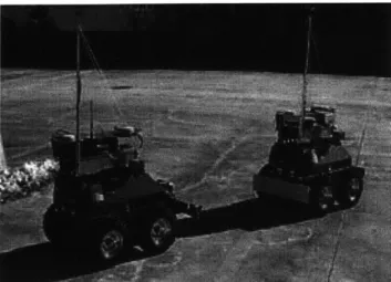
1-2 Ground exploration vehicles at the Aerospace Controls Lab, MIT . . . . 19

2-1 The Update Step as it should occur (left), and as it actually occurs (right). The curved line is the level line of the range measurement: on this line, the range is constant. . . . . 24 2-2 The divergence of the EKF when all three divergence factors are present. On

the left, range measurement is much more accurate than the bearing measure-ment. On the right, the bearing measurement is much more accurate than the range measurement . . . . 25 2-3 The range p is large, making the B term small. The performance of the EKF

and GSF does not differ much, even though the measurements still have a large difference in their noises. . . . . 32

2-4 Performance of EKF, GSF and Bump-up R methods with o = 100. The GSF

and Bump-up R methods perform much better than the original Extended K alm an Filter. . . . . 37

2-5 The divergence of the EKF when all three divergence factors are present(bearing measurement error is much larger than range measurement error). On the left, the graph shows the estimation error for three different filters. On the right, the condition number for P is plotted. . . . . 39 2-6 The divergence of the EKF when all three divergence factors are present (range

measurement error is much larger than bearing measurement error). On the top, the graph shows the estimation error for three different filters. On the bottom, the condition number for P is plotted . . . . 41

2-7 The convergence of the EKF when measurement noises are of the same order of magnitude (not all divergence factors are present). On the top, the graph shows the estimation error for three different filters. On the bottom, the condition number for P is plotted . . . . . 42

2-8 On the top: the effect of varying the HPHT bump-up term when U0 = 20.

The HPHT term is multiplied with constant a = 1, 2.. .7. The best accuracy

is achieved with a = 4. On the bottom: The effect of varying the HPHT bump-up term. In this case, ao = 10. The HPHT term is multiplied with

constant a = 1, 2... 7. The best accuracy is achieved with a = 6. . . . . 44

2-9 The effect of multiplying HPHT term with a positive constant a . . . . 46 2-10 The performance comparison of the regular, continuous Bump-up R method

and the Two-Step method with the EKF method starting at time step 15. The EKF alone, without the Bump-up R "help", diverges . . . . 47

intro-3-2 Error Covariance Comparison. Differences between the various covariances are all non-negative, which means that P+ > P+ > .+. ... 57 3-3 LJ " as a function of R; When R = 1, then P+ = P+ and the

dif-ference is largest. On the other hand when Rbu ~ Rf then Rbu

<

3-4 Error Covariance Comparison. This figure actually shows what this section has proven: Paf > Pabu > Pbest > Pbu > Pf. The bump-up terms in Bump Up R/SK filters are bringing the Paf and Pf to new values Pabu and Pbu which are closer to the best possible covariance value Pbest . . . . 65

4-1 Profile of the simulation with 16 vehicles. It shows the "take-estim" function as one of the most computationally demanding functions (dark color means the computations are actually performed inside the function as opposed to inside the sub-functions) . . . . 74 4-2 Performance comparison of the decentralized algorithms with and without

com munication delay . . . . 76

4-3 Hierarchic Clustering. Super Cluster and the sub-clusters may run different estim ation algorithm s. . . . . 79

4-4 The comparison of various architectures: centralized, decentralized, HCC and

HCD. The range of vehicles used in this comparison is from 4 to 25 spacecraft 87

4-5 The comparison of the two hierarchic estimation architectures. The range of vehicles used in this comparison is from 16 to 50 spacecraft . . . . 90

4-6 Probability distribution of communication delay . . . . 93

4-7 The performance comparison of various filters when communication delays are introduced... ... 102

5-1 SPHERES satellite . . . . 106 5-2 SPHERES 2D test at the MSFC . . . . 107

5-3 Schematic of SPHERES lab (2D) space, with four beacons mounted on the

w alls . . . . 108

5-4 Receiver triggering schematics. The threshold is raised to a certain level in order to filter the noise. . . . . 116 5-5 Error graph, from Serge Tournier (1 beacon, 2 receivers, same beacon-receiver

configuration) . . . . 117 5-6 Standard deviation graph, from Serge Tournier (1 beacon, 2 receivers, same

beacon-receiver configuration) . . . . 118 5-7 3D setup (with z component constant) with 2 beacons and 4 receivers on a

single SPHERES face . . . . 119

5-8 Evolution of error in beacon positions . . . . 128 5-9 Performance of the proposed calibration approach. The "x" are true positions

Chapter 1

Introduction

Future formation flying missions are being planned for fleets of spacecrafts in MEO, GEO and beyond, where relative navigation using GPS would either be impossible or insufficient. To perform fleet estimation for these scenarios, local ranging devices on each vehicle are being considered to replace or augment the available GPS measurements. 1-1 Besides being identified as an enabling technology for many types of space science missions [9], the concept of formation flying of satellite clusters has also been identified as one of the enabling tech-nologies for the NASA exploration initiative [10]. Examples include ground-exploration in remote destinations where vehicles have to work together to be more efficient than a single vehicle 1-2.

The use of many smaller vehicles instead of one monolithic vehicle can have several benefits:

" improving the science return through longer baseline observation. " enable faster ground track repeats.

" provide a high degree of redundancy and reconfigurability in the event of a single

vehicle failure.

Figure 1-1: A fleet of spacecraft in deep space with relative ranging and communication capabilities

However, the guidance and navigation system for these large fleets is very complicated and requires a large number of measurements. Performing the estimation process in a centralized way can lead to a large computational load that can make the system unusable. Therefore, there is a need for distributing the computational load using decentralized or hierarchic estimation architectures.

This work will focus on extending the previous work of Plinval [1] and Ferguson [22]. It will also provide the analysis that shows the benefits of using Schmidt-Kalman filter as a choice for decentralized estimators.

In addition to this topic, two more ideas will be explored. The first is the analysis of EKF divergence in the presence of so-called divergence factors such as non-linearity in measurements with distinct accuracies and large initial co-variance.

Figure 1-2: Ground exploration vehicles at the Aerospace Controls Lab, MIT

beacon position calibration technique for SPHERES will be introduced and presented as a part of the chapter. This technique will show a simple estimation approach in determining the beacon positions in the SPHERES test environment, which would provide great flexibility for the SPHERES system.

1.1

Thesis Outline

This thesis consists of six chapters. After the initial introduction, the second chapter will focus on the divergence issues with the extended Kalman filter. Previous work will be briefly described, followed by new insights and simulations.

Chapter 3 examines the analysis of decentralized estimation filters for formation fly-ing spacecraft, in which bump-up decentralized algorithms (more specifically, the Schmidt-Kalman filter) are shown to have an advantage over the non-bump-up estimators. The analytical derivation is shown, followed by the simulation results.

Chapter 4 describes the various estimation architectures and compares them against

eral different metrics. This, in essence, is a continuation of the work done by Plinval [1} with an improved simulator. A brief, qualitative discussion of robustness of various estimation architectures is included.

Chapter 5 describes the measurement bias problem in SPHERES and potential ap-proaches to solve it. However, the specific nature of the biases in the SPHERES measurement system creates a much more complex problem, which cannot be solved easily and efficiently using estimation techniques. This chapter also describes the SPHERESs beacon position calibration technique, which allows the SPHERES system to be more flexible when changing test environments.

Chapter

2

Mitigating the Divergence Problems

of the Extended Kalman Filter

2.1

Introduction

The Extended Kalman Filter (EKF) is the most common non-linear filter for estimation problems in the aerospace and other industries. The EKF performs very well in solving problems with non-linear measurements and/or non-linear dynamics. However, the filter is not optimal due to the approximation that is performed using the linearization method (i.e. Taylor series expansion). This linearization can also cause undesirable effects on the performance of the filter [3, 4]. We will consider how the EKF can diverge when applied to a system with a large initial state-error covariance that uses non-linear measurements of distinct accuracies [1].

The EKF divergence issues are well known and documented [3, 4, 5, 6]. Several studies have already described the causes of divergence in the EKF for relative navigation

lems [8, 22, 25]. The recent work of Huxel and Bishop [8] addresses the divergence issue of EKF in the presence of large initial state-error covariance,inertial range (large p) and relative range (small p) measurements. They concluded that EKF divergence is caused by ignoring the large second order linearization terms in B that correspond to relative (short) range measurements. The B term is included in the Gaussian Second Order Filter (GSF), which allows the GSF to converge. Because the measurements used in their analysis were of equal accuracy, they did not explore the effect on the system when some measurements had different accuracies than others. Plinval [1] described the effect of using sensors with different accuracies on the performance of the EKF. He geometrically explained the reason behind the divergence of EKF when the non-linearity in the sensors is coupled with their different accuracies. This chapter will extend that analysis to show that the EKF can have divergence issues when three different divergence factors are combined (see Problem State-ment). We will also provide a more general discussion of the problem presented by Plinval and introduce two methods (GSF and Bump-up R) to address the problem.

2.2

Problem Statement

As discussed in Ref. [1], the problem of EKF divergence due to non-linear measurements of substantially different accuracies can be explained geometrically. The problem lies in the process of linearizing the non-linear measurements, in which some information is lost. This means that in every subsequent step, the measurement matrix H in the EKF measurement update equation is incorrect. This error can become even more significant during the es-timation process if the measurements being linearized have different accuracies. However, for this effect to actually become significant, the filter needs to rely mostly on the measure-ments. This will be the case if there is a large initial state-error covariance P. Therefore,

" Large initial state-error covariance PO. Large means much larger than measurement noise covariance R.

" Significant non-linearity in measurements. " Large difference in the measurement errors.

2.2.1

Problem Walkthrough

Let us consider a system where a state vector of size 2 is estimated using non-linear sensors of significantly different accuracies and with poor initial knowledge of the states (i.e. large

Po). This is similar to the system used in Ref. [1]. After the first measurements are collected,

the state error covariance matrix P can be updated as

P+ = (I - KH)P~ (2.1)

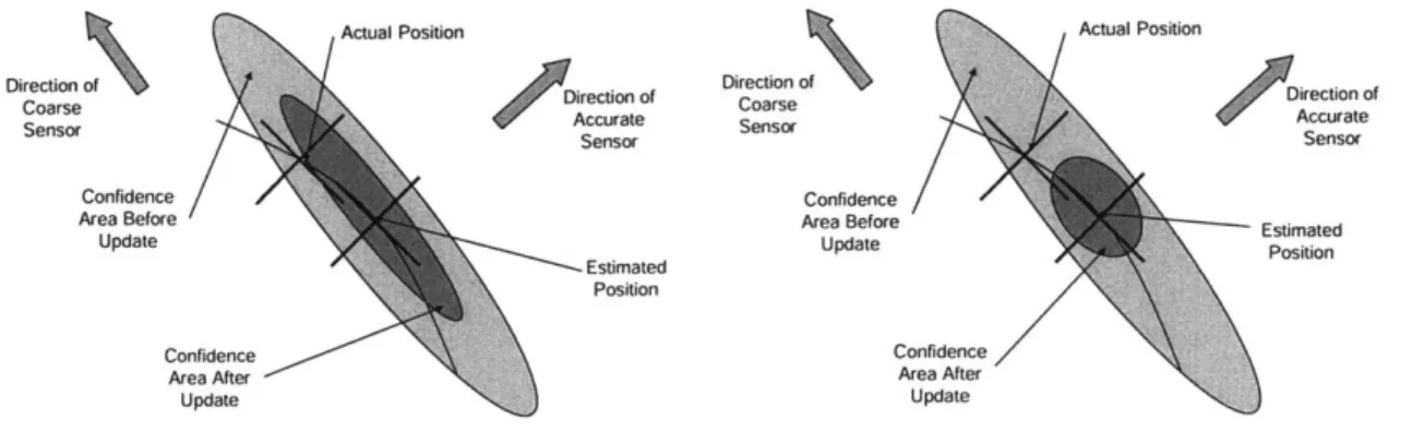
Since Po is large, the filter will give preference to the measurements rather than the previous knowledge. After the first update, the state error covariance matrix will have a very small eigenvalue in the direction associated with the more accurate measurement. However, it will still have a large eigenvalue in the direction associated with the less accurate measurement. The new measurements collected after the first update will now be linearized around the newly acquired estimate. This means that the directions of the linearized new measurements will be different from the directions of the previous measurements. During the second update, the more accurate measurement will cause a further decrease in state error covariance in the direction corresponding to that measurement. However, this direction is not the same as in the previous update step. This can lead to a significant decrease in the state error covariance in a wrong direction. This can be observed in Figure 2-1. Furthermore, as the state error covariance matrix, P, decreases in directions other than the ones corresponding

Actual Position Actual Position

Dirction of Direction of Direction of Direction of

Sensor Accurate Sensor Accurate

Sensor Sensor

Confidence Confidence

Area Before _{Area Before}

Estimated Update _Update Positon Estimated Position Confidence Confidence

Area After Area After

Update Update

Figure 2-1: The Update Step as it should occur (left), and as it actually occurs (right). The curved line is the level line of the range measurement: on this line, the range is constant. to the direction of the accurate measurement, the EKF will become decreasingly responsive to measurements in those wrong directions and it will become increasingly confident in its prior state knowledge. If the state error covariance becomes sufficiently small with the state estimates still far away from the true state, the EKF will diverge. This phenomenon is called spill-over of good measurements in the wrong directions.

2.2.2

Divergence due to Three Divergence Factors

In the problem statement, we referred to the three factors that are responsible for the divergence of the EKF. Of course, it is possible to have divergence with only two of those factors, especially when highly non-linear measurements are involved. However, when all three factors are included, the EKF can diverge easily. In order to confirm this, we will show a series of simulations with various factors included in the simulation section. The simulations will show that when one of the factors is accounted for or is minimized, the EKF will converge.

Plot of Estimation Error 12 40-10 E E 30-tU'6 8- L 6- 201 k to-2 41 2- 10 0 5 10 15 20 0 5 10 15 20 iterations iterations

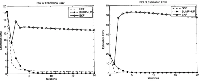
Figure 2-2: The divergence of the EKF when all three divergence factors are present. On the left, range measurement is much more accurate than the bearing measurement. On the right, the bearing measurement is much more accurate than the range measurement

Figure 2-2 shows the performance of the three different filters, EKF, GSF and Bump-up

R when all three divergence factors are present (the details of these simulations are given in

the Simulation section, 2.4). That is: the EKF filter diverges when non-linear measurements of highly different measurement noises are used for updating the system with large Po.

The performance of the GSF and Bump-up R filters is also shown in Figure 2-2. Their performance is superior to the performance of the EKF filter, as they are accounting for one of the three divergence factors. This will be examined in the following sections.

2.3

EKF, GSF and Bump-up R Algorithms

This section will focus on the derivation of the three filters. We will use the system similar to the one described in chapter 6 of [1]. The system is in 2D, and we are trying to estimate the position of the fixed object using two non-linear measurements: range and bearing. In addition, we will use the scalar update approach to show the evolution of the B term

25

described in the GSF algorithm. System state model is as following:

Xk

Xi1

2

-k

where the states: x1 = x, X2 = y, are coordinates of the fixed object

Xk+1

[

k

-[

+4

Setting the process noise w to zero and using the fact that, in order to simplify the analysis, there are no dynamics

AXk = 0 => xk+1 = zk and xk+1 = X k (2.4)

or equivalently that

41

simplified to

P4+1 = Pk+ (2.5)

This allows us to focus on the measurement update equations. The non-linear range and bearing measurements can be written as:

h1= p =

+

h2=6

arctan

(-)

with corresponding Jacobian:

±1 -x 2 2 22 2

I

The measurement accuracy is:

(2.9) o o2

where o- and of are range and bearing measurement noise covariances, respectively. The initial conditions are:

x1 = X0 x2 =o PO = 0 0o 2 (2.10) (2.11) (2.12)

I

Having all the initial values, we can proceed with analyzing different filters. The analysis of the EKF and its related divergence problem is closely tied to the results obtained for the

GSF case, so only the GSF analysis will be presented.

2.3.1

Gaussian Second Order Filter

the measurement update equations for the Extended Kalman Filter (EKF) and the Gaussian Second Order Filter (GSF) [?) are:

K = P-HT (HP--HT + R) 1 fo

K

P-HT (HP-HT + R +

where B is the covariance term due to the second order terms. B is calculated using Hessians

H' and H2, by calculating each member of matrix B separately:

1

Bik =

trace(H'P-HP-)

Hessians H' and H are defined as second order derivatives of measurement functions hi and

h2. Note that the Hessian of h is a tensor: 02 hi (k) H= O 2 H' ₂ =0 2_aiCh2(i)2 (2.16) (2.17)

In this case H' and H2 are:

x 2 X P3 _p P3_p 4 -p 4

I'2

I

4

go0

2

Up4

I

(2.20)

Using the initial value of B, P, H, and R, we can proceed and calculate the B term after the first update step. To do this, we will perform the first measurement update step on the

GSF, one measurement at the time (scalar update approach [81). We will then apply the

-approximation used by Huxel and Bishop [8], to obtain bounds for B:

1

0 < Bh:h

< -(lDhl|trace(P~))

2 (2.21)

where Bhkk corresponds to B, and Dh corresponds to Hessian in our case. Performing the measurement update with the first (range) measurement:

(2.22)

P

Where H1 corresponds to the first row of the Jacobian matrix H. Therefore:

H₁PoHi

-[

~]

[

1

[

= B1 1, as calculated earlier in equation 2.20. In order to compute the bounds on

B we need to calculate the trace(P). Therefore, the elements on the main diagonal of the

state error covariance matrix pu and p+ can be calculated as:

P+ = (I

-

p = _{oo1 (2.28)}

(1 2 00- + U 2 + 4)

+ = a 1 - _(2.29)

P22 _{0 2 (2}

+ U2 +

Simplifying the expressions for pn and p2:

h= 1 (2.30) p2

(0-

/

and the similar result (using x2 instead of 1) can be obtained for p2 after the update with

the first measurement. A detailed analysis of equation 2.32 reveals several key properties for various important cases. For example, depending on the relative values of o-o, u, and p, the expression 2.32 will show what influences p+ and p+ the most. The range p plays an important role in determining the significance of non-linearities in measurements. Therefore, we will observe two different cases with respect to the size of p:

* P > go > 07p

0e- ~ -o >a p

Case 1: p > uo >

o-In the first case, p

>

>

(22

A similar expression can be obtained for p2. This expression shows that for a large range, p, the p' term is very small. This is as expected, since when the state error covariance is relatively large compared to the measurement error covariance, the Kalman filter will mostly rely on the new information coming from the measurements, rather than on the previous information. After using the same approach for the second measurement, and applying the equations 2.5 and 2.21, similar results were reached, which were confirmed in the simulations

(I|BII

It can be concluded that the compensation term due to the non-linearities in the mea-surements, B will be very small, and as stated in 2.21 the non-linear effect of measurements will be small. The initial B shown in the equation 2.20 is also very small due to large p. This means is that the large p diminishes the non-linear effect of the non-linear measurements. Therefore, the large p can account for one of the divergence factors and EKF can converge, as shown in Figure 2-3. (Large number (50) of initial conditions were tested and Figure 2-3 is a representative sample.)

Case 2: p ~~ Oo

>

The previous case has shown that the compensation term B may not have a large effect on the performance of the EKF filter when p is large. However, in this case, p is of the same order of magnitude as o-o. The equation 2.32 can not be approximated as in the previous case and it remains:

pii =- 2 +U2 (2.34)

O 2p2

Estimation Error 12-w C . 10-E c8-6 4 - 2-0 0 5 10 15 20 iterations

Figure 2-3: The range p is large, making the B term small. The performance of the EKF and GSF does not differ much, even though the measurements still have a large difference in their noises.

Therefore, according to Eq.2.21, the linearization compensation term B will become signif-icantly larger than in Case 1. Of course, this is expected since the non-linearity becomes significant for small ranges, and the second order terms compensated by B can not be ignored anymore without risking the divergence of the filter.

GSF Analysis Conclusion

The two cases clearly show an important trait: when P is relatively large compared to R, and the range p is of the same order of magnitude as P, then the B term becomes important in order to prevent the EKF from diverging, by avoiding the "spillover" effect discussed earlier. If p is much larger than the other values, the EKF can converge even without the use of B.

The reason is that the non-linear effects of the measurements are not significant, as shown earlier in the discussion of Case 1.

Also, when P is small enough op

>

P = o2 (2.35)

Again, there is no need for the compensation term B, by using the same reasoning as in Case 1.

Since P is usually large initially, it can be concluded that bringing P down slowly by some estimation method other than EKF and then allowing the EKF to take over, as shown in Section 2.4.4, can be beneficial. Of course, there are other ways of solving the diver-gence issue with EKF, namely the Bump-up R method. However, the true benefit of the

GSF and the analysis shown above is to explain how the measurement errors coupled with

the non-linearities and large state error covariances can have a negative effect on the filter performance.

2.3.2

Bump-up R method

This method has been shown to be an efficient way of fixing the problem of EKF divergence. The main idea behind the bump-up R method is to set the measurement error covariance R to a value somewhat larger than the original measurement noise in order to compensate for the non-linearities and differences in the measurement noises among various measurements [7]. As proposed in the Ref.( [1]), the bumping-up term Rbump that will successfully resolve the divergence problem is:

Rbmmp = HP-H T (2.36) 33

Rnew = R + Rbump

Plinval further explained how this specific form of Rbump actually helps. As shown earlier, the reason why EKF does not converge is explained by the reduction of the state error covariance in a wrong direction after the measurement update. By keeping the measurement error covariance large, this fast reduction is not permitted, but rather the reduction occurs much slower. Ultimately, the goal is to reach a small enough state error covariance P, after which, as shown by Case 2 of the GSF analysis, the filter will not rely on the measurements to the same extent that it does initially (when the P was large).

According to Plinval [1], this form of Rbump is selected because it allows the accuracy of the sensors to follow the evolution of the state error covariance P, thus preventing P from becoming ill-conditioned. He shows that this approach slows down the convergence of the filter, but also prevents the divergence, by preventing the over-reduction of P in the direction of the coarse sensor. In fact, the Bump-up R method increases the measurement error covariance, R, so that the filter does not rely solely on the measurements (which, due to their non-linearity, are less accurate than expected) but also on the previous knowledge. Essentially, the Bump-up R method eliminates one of the three divergence factors: Uo

>

This approach has also been used by Huxel and Bishop [8], with the same Rbump term but without the analytic explanation offered, for solving navigation problems involving large state error covariances P and ranging measurements of different orders of magnitude. It was shown that these types of problems can also cause divergence of the EKF, and that the above mentioned Rbump term can avoid it. The simulation results will further confirm the

benefits of this approach.

Bump-up R Analysis Conclusion

It is interesting to note that the compensation term B in the GSF analysis also behaves as the bump-up term. The main difference is that B is actually computed as the compensation for the second order terms in the Taylor series expansion, that were initially ignored in the EKF approach. The Rbump term is an artificial way of slowing the reduction of P, which was analytically shown in [1]. It makes the measurement noise larger, in order to prevent the filter from focusing too much on measurements. Since both terms yield similar results, in the simulation section we will explore how some other similar bump-up terms perform in attempt to prevent the divergence of EKF. Also, it is important to note that the computational load for calculating B is larger than that for Rbump, since B is calculated using Hessian tensors of measurement functions h.This makes the Bump-up R method better for practical purposes. The simulations will also show that the bump-up R method tends to be the more accurate

of the two methods.

2.4

Simulation

The simulation section will present the performance of the various methods mentioned in this chapter. First, we will describe the system that will be used for simulation. In addition, the results generated with different methods and different initial conditions will be presented. This will include the performance of EKF, GSF and Bump-up R methods; the effects of varying bump-up terms; and a two-step method. Finally, conclusions will be drawn to state how well the simulated results follow the analytical.

2.4.1

Plinval's Example revisited

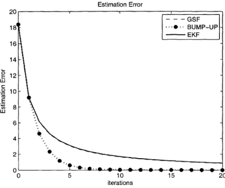
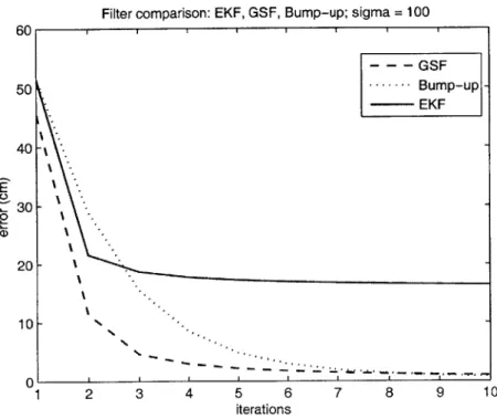
In the work published by Huxel and Bishop [8], the divergence of EKF was observed when the system involved the measurements whose order of magnitude was of the same order as the state error covariance. Plinval ([1], Chapter 6) described the divergence of EKF in the presence of non-linear measurements with very different measurement noises. Fig. 2-4 shows the example examined by Plinval, and it clearly presents the advantages of GSF and Bump-up R methods over the EKF. The GSF method converges faster, but eventually the Bump-up R method reaches the same and even better accuracy. In this case, the initial state error covariance (Po) and measurement error covariance (R) are:

1002 0

PO

0

Also the initial position estimate was set at:

20

xIi = (2.40)

80

Since, in this specific case, the range is of similar order as the state error variance p 141.4 and oo = 100, this example clearly shows the divergence effect when all three divergence

factors are involved. Also, it shows the convergent behavior of the two methods, the GSF and the Bump-up R. Plinval has also has shown that this is true for a large number of initial conditions.

Filter comparison: EKF, GSF, Bump-up; sigma = 100 30 0 0 1 1 1 1 1 1 2 3 4 5 6 7 8 9 10 iterations

Figure 2-4: Performance of EKF, GSF and Bump-up R methods with oo = 100. The GSF and Bump-up R methods perform much better than the original Extended Kalman Filter.

2.4.2

The Simulated System

The simulated system is similar to the system described by Plinval ([1], Chapter 6). The equations are already included in the Analysis section (Eqs. 2.2 - 2.12). In order to focus on the effects of the measurements on the performance of the filter, the target has a fixed position and the non-linear measurements involved are range and bearing from the coordinate center. The true position of the target is at:

1001

Xtruth = (2.41)

100

The initial position, state error covariance and the relative size of measurement noises will vary. Since the measurements are of different types, the order of magnitude of the mea-surement noise is not the most representative way of comparing the accuracies of these two measurements. In general the measurement noise in the bearing angles can be much more significant than the ranging noise, especially if the range is of large magnitude.

Performance of EKF, GSF and Bump-up R methods

For Figures 2-5 - 2-7, the plots on the top show the performance of the three filters discussed in this chapter. The plots on the right show the conditional number P, which is identified as one of the symptoms of divergence (or convergence) by Plinval [1]. Different divergence factors are introduced or removed. For example, the plots on the top in Figures 2-5 and 2-6 show the performance of the filters when there is a significant difference in the errors of the two measurements. In both cases, p is comparable in size to Uo, which is much larger than the measurement errors. This combination of the three divergence factors leads to an ill-conditioned P matrix, and may lead to divergence [1].

The Gaussian Second Order filter accounts for the non-linear effect of the measurements, which effectively removes one of the divergence factors. This translates directly to the convergence of GSF. Cond(P) is kept low in the initial steps, which was sufficient enough time to allow the filter to converge and avoid significant spill-over.

The Bump-up R method converges somewhat more slowly than the GSF, since it degrades the accuracy of the measurements by a much larger amount than B. This, as described earlier, prevents the filter from focusing too much on measurements, which leads to slower convergence. In the steady-state, the Bump-up R method actually performs better than

Plot of Estimation Error 0 5 10 15 iterations 14 212 0 -o 10 E 6 4 2 0 10 0 5 10 15 iterations

Figure 2-5: The divergence of the EKF when all three divergence factors are present(bearing measurement error is much larger than range measurement error). On the left, the graph shows the estimation error for three different filters. On the right, the condition number for P is plotted. 20 18 16 Plot of cond(P) *0 C 0 0 20 20 10 4 10 3 10 2 1 1

Table 2.1: Computational load for the EKF, GSF and Bump-up R methods

Method _{EKF GSF Bump-up R} Computational load (ms) 0.13 0.29 0.13

Figure 2-7 shows the performance of the three filters when the measurement errors are of the same order of magnitude. The EKF in this case converges since not all three divergence factors are present. This effectively confirms our hypothesis that the three factors described in this chapter can easily lead to divergence. Again, the Bump-up R method converges somewhat more slowly than the GSF. The plot of cond(P) shows that all three filters keep the P well-conditioned, which in this case translates to convergence.

Computational Load

While the first few simulation results show the superiority of the GSF and Bump-up R methods over the Extended Kalman Filter, it is also of great importance to see how practical these methods are. The EKF is widely used, as it can be easily and efficiently implemented on the computers. Table 2.1 shows the computational load of each of the methods while running on the Pentium IV, 2.6GHz processor. The EKF and Bump-up R methods perform better than the GSF method because they does not require the computation of the Hessian tensors of the measurement functions h, that are required for GSF. The EKF and Bump-up R have about the same computational effort, since the bump-up term in Bump-up R method,

Plot of Estimation Error 70 0 L-J C 0 E Co 104 iterations Plot of cond(P) 10 iterations

Figure 2-6: The divergence of the EKF when all three divergence factors are present (range measurement error is much larger than bearing measurement error). On the top, the graph shows the estimation error for three different filters. On the bottom, the condition number for P is plotted. 41

Plot of Estimation Error iterations Plot of cond(P) V C 0 C.) 100 0 2 4 6 8 10 12 14 16 18 20 iterations

Figure 2-7: The convergence of the EKF when measurement noises are of the same order of magnitude (not all divergence factors are present). On the top, the graph shows the

20 1 1 14 " 12 W 10 C8 E w-0

2.4.3

The Effect of Varying the HPHT Bump-up Term

As presented in the analysis section, the term B that appears in the derivation of the Gaussian second order filter behaves similarly to the HPHT term in the Bump-up R method. The previous figures show that these two approaches also prevent the extended Kalman filter from diverging. Therefore, it is of some interest to see how small variations in the HPHT term can affect the performance of the Bump-up R method.

Figure 2-8 shows the effect of multiplying the HPHT term in the Bump-up R method with a constant. On the top is the plot when the initial state error standard deviations are set to 20. In the steady-state, it can be seen that the performance of the original Bump-up

R method with the HPHT as a bump-up term performs worse than the methods in which

the HPHT term is multiplied by the constant. In this specific case, the best accuracy is achieved when the multiplier a = 4. For a > 4 the accuracy degrades. The plot on the bottom in Figure 2-8 shows that the performance of the Bump-up R methods with the varying multipliers (a) actually depends on initial conditions. For the case of o-o = 10, the

best performance is achieved with the multiplier a = 6. The improvement observed by multiplying the HPHT term with a constant is very small, but it shows that there is a limit to how far the bumping-up method can go. When a is set to a very large number (i.e. 100 or 1000) the Bump-up R method consistently diverges, similarly to EKF, for various initial conditions.

On the other hand, the plots in Figure 2-9 show the effects on performance of a filter when the HPHT term is multiplied with a constant a > 1 and 0 < a < 1. Figure 2-9

demonstrates that all three of the bump-up R methods solve the divergence problem of the EKF. The only significant difference among the Bump-up R methods is observed in the bottom plot of Figure 2-9, where the steady states are compared. This figure shows that

INIT: x = 87, y = 113, sigma = 20 0.065- 0.06-alpha=1 -0 alpha=2 0.055- - - - alpha=3 - B - alpha=4 - + -alpha=5 E 0.05-- * -alpha=7 o 0.045a-0.04-_.0 ... 0 ... ... ... 0 0.035 - - - - - - .x - .-. -. - ---197.5 198 198.5 199 199.5 200 iteration INIT: X = 94, Y = 106, SIGMA = 10 0.16---- alpha = 1 -e - alpha = 2 0.14- - - alpha = 3 -S - alpha = 4 -+ - alpha = 5 E 9 0.12 -- alpha = 6 0.12-P- - alpha = 7 0.1 ---- - - - ---

8-

-o

Figure 2-8: On the top: the effect of varying the HPHT bump-up term when -0 20.

when the HPHT term is decreased, the steady state performance of the filter degrades.

2.4.4

The Two-Step Approach

The Two-Step method mentioned in the analysis section originates from the observation that the EKF filter will not diverge when initial state-error covariance is low (or in other words, when there is a high confidence in the initial state of the system). A similar observation was made by Huxel and Bishop [8]. In essence, this method effectively removes one of the divergence factors (large Po) and allows the EKF to converge.

The Two-Step method is not a new concept. It has been explored by Kasdin [2] and discussed in technical comments by Lisano [7]. The basic idea is to bring the initial state error covariance to a sufficiently low level so that the EKF can take over the estimation process, which then will not lead to divergence. Based on the results presented in this chapter, it can be seen that one way of fulfilling the requirement of lowering the state-error covariance is by running the Bump-up R filter during the first few time steps. Following that, one can switch to using the EKF. Figure 2-10 demonstrates this case. This figure compares the performances of the regular Bump-up R method that runs continuously versus the Two-Step method, in which the EKF method starts at time step 15. The EKF converges very well, and its performance is almost as good as the performance of the Bump-up R method.

2.5

Conclusion

This chapter examined the divergence issue of the Extended Kalman Filter (EKF), which occurs in the presence of non-linear measurements with large accuracy differences and large initial state-error covariance. Indeed, the analysis presented here has shown that the

14 12 - alp = 1 ... - alp = 2 10 8 0 a> 6 4 2 -0 0 50 100 150 200 iterations 0.6 - - - alp = 0.1 . - alp = 1 ... alp=2 0.5-0.4 - - - - - - - - - - - - - - - - - - - - - - - - -0.3- -" 0.2 -a> 0.1 - 0--0.1 - -0.2-175 180 185 190 195 200 iterations

Two-Step 2-a) C C E 4- 2-0 ' - - - - - -0 50 100 150 200 iterations

Figure 2-10: The performance comparison of the regular, continuous Bump-up R method and the Two-Step method with the EKF method starting at time step 15. The EKF alone, without the Bump-up R "help", diverges

vergence of the EKF depends on a combination of factors: the size of the initial state error covariance, P, the relative sizes of the measurements noises and the non-linearity of those measurements. This is also confirmed by Plinval [1], with the use of a geometric argument. The basic idea is that the initial state error covariance needs to be large enough to allow the filter to focus on the measurements. These non-linear measurements are highly dependent on the state estimates, as their linearization is performed in the vicinity of those estimates. Those state estimates can be far off as a result of the spill-over effect described in the Prob-lem Statement section of this chapter and also in [1]. This combination may lead to filter over-reliance on the measurements that are actually less accurate than what their measure-ment noise covariance shows. As the process iterates based on these corrupt measuremeasure-ments, the EKF can diverge.

A couple of methods have been presented that seem to solve the divergence problem of

the EKF. The Gaussian second order filter (GSF) includes the second order terms from the Taylor series expansion (which are ignored by the EKF) and therefore somewhat accounts for one of the factors responsible for the divergence. These second order terms are represented in the filter equations as a compensation or as a bump-up term B. This term is added to the measurement noise covariance, R. The simulations show that this effectively improves the convergence of the filter. However, this method is of less practical value as it is accompanied

with a large computational load.

Another way of solving the divergence problem is by developing another bump-up term,

HPHT. Again, this term is added to the measurement noise covariance, R. Similarly to the

GSF method, this bump-up term makes measurements less accurate and diverts the filter's

attention away from the measurements. This method is more practical, as the computational load is comparable to the one of EKF. Although the convergence is shown to be a bit slower than in the case of the GSF, it is still sufficiently fast. The effect of varying the HPHT term is also presented in the Simulation section.

Finally, the Two-Step method is presented as the combination of the Bump-up R method and the EKF. The purpose of the Bump-up R method is to bring the error covariance P to a low value, after which the EKF can continue without diverging. The reason is that when

P is low, the EKF does not rely on the measurements as much. Essentially, this removes

Chapter 3

Analysis of Decentralized Estimation

Filters for Formation Flying

Spacecraft

3.1

Introduction

The concept of formation flying of satellite clusters has been identified as an enabling tech-nology for many types of space missions [9], [10] '. In the near future, some formation flying technologies may fit well into the new NASA initiative. An example of this is ground explo-ration of remote destinations, where having a group of vehicles working together may be far more efficient than a single vehicle. The use of fleets of smaller vehicles instead of one mono-lithic vehicle should (i) improve the science return through longer baseline observations, (ii) enable faster ground track repeats, and (iii) provide a high degree of redundancy and recon-figurability in the event of a single vehicle failure. The GN&C tasks are very complicated

'This chapter has been pubished at the AIAA GNC conference, August 2004 [24]

for larger fleets because of the size of the associated estimation and control problems and the large volumes of measurement data available. As a result, distributing the guidance and control algorithms becomes a necessity in order to balance the computational load across the fleet and to manage the inter-spacecraft communication. This is true not only for the optimal planning, coordination, and control [11], but also for the fleet state estimation, since the raw measurement data is typically collected in a decentralized manner (each vehicle takes its own local measurements).

GPS can be used as an effective sensor for many space applications, but it requires

con-stant visibility of the GPS constellation. In space, GPS visibility begins to breakdown at high orbital altitudes (e.g. highly elliptic, GEO, or at L2). Thus, a measurement augmen-tation is desired to permit relative navigation through periods of poor visibility and also to improve the accuracy when the GPS constellation is visible [13, 14, 15, 16, 17].

However, the local range measurements taken onboard the spacecraft strongly correlate the states of the vehicles, which destroys the block-diagonal nature of the fleet measurement matrix [12, 18] and greatly complicates the process of decentralizing the algorithms [20]. In contrast to the GPS-only estimation scenario, which effectively decentralizes for reasonable fleet separations, this estimation problem does not decorrelate at any level. As a result, Ref. [20] investigated several methods to efficiently decentralize the estimation algorithms while retaining as much accuracy as possible.

To populate the decentralized architectures, Ref. [20] developed a new approach to esti-mation based on the Schmidt Kalman Filter (SKF). The SKF was shown to work well as a reduced-order decentralized estimator because it correctly accounts for the uncertainty present in the local ranging measurements, which is a product of not knowing the loca-tion of the other vehicles in the fleet. Since this correcloca-tion is applied to the covariance of

(SCC).

We extend the covariance comparison in Ref. [20] to consider the transients that occur as ranging measurements are added to the estimator. Ref. [201 performed a similar compar-ison on the steady-state covariances from the various filter and architecture options. This enabled a comparison of the filter performances, but it could not explain why some of the decentralized techniques performed better than others. The investigation in this paper of what we call the "transient response" of the filter provides further insight on the relative performance of these filters. This analysis also indicates the advantage of using the SCC, which can be extended to other estimation algorithm/architectures.

The following section discusses prior work on reduced-order decentralized filters, which is followed by a detailed investigation of the covariance for different algorithms.

3.2

Reduced-order Decentralized Filters

Recent work by Park [21] introduced the Iterative Cascade Extended Kalman Filter (ICEKF), a reduced-order estimation algorithm for use in decentralized architectures. This filter is used for local ranging augmentation in applications where GPS-only measurements are not suffi-cient. The ICEKF filter uses an iterative technique that relies on communication between each vehicle in the fleet and continues until a specified level of convergence is reached. It was shown that the ICEKF can incorporate local ranging measurements with GPS levels of accuracy, producing nearly optimal performance. However, Ref. [22] demonstrated that the filter performance can deteriorate when highly accurate local measurements (i.e., more ac-curate than GPS) are added, and that this performance loss occurs when error/uncertainty in the relative state vectors is not correctly accounted for in the filter.

One way to account for this uncertainty in the relative state is to include it in the measurement noise covariance R, which is the approach taken in the Bump Up R method:

Rbump = R + Jyy jT (3.1)

where J is the measurement matrix for all non-local measurements in the fleet and Pyy is the initial covariance matrix for all non-local states in the fleet state vector. Equation 3.1 implies that the measurements now have larger noise covariance, making them less accurate than was initially assumed.

Another approach examined in Ref. [22] is the Schmidt Kalman Filter (SKF). This filter also increases the variances in the R matrix, but in contrast to Bump Up R, this approach is dynamic and also accounts for the off-diagonal blocks of the error covariance. The SKF eliminates non-local state information, thereby reducing the computational load on the pro-cessor. This elimination is accomplished by partitioning the measurement and propagation

equations: [ Ox2

]k[Ylk

P

1