HAL Id: hal-00317327
https://hal.archives-ouvertes.fr/hal-00317327
Submitted on 8 Apr 2004
HAL is a multi-disciplinary open access
archive for the deposit and dissemination of
sci-entific research documents, whether they are
pub-lished or not. The documents may come from
teaching and research institutions in France or
abroad, or from public or private research centers.
L’archive ouverte pluridisciplinaire HAL, est
destinée au dépôt et à la diffusion de documents
scientifiques de niveau recherche, publiés ou non,
émanant des établissements d’enseignement et de
recherche français ou étrangers, des laboratoires
publics ou privés.
at low and mid latitudes from WINDII and potassium
lidar observations
M. Shepherd, C. Fricke-Begemann
To cite this version:
M. Shepherd, C. Fricke-Begemann. Study of the tidal variations in mesospheric temperature at low
and mid latitudes from WINDII and potassium lidar observations. Annales Geophysicae, European
Geosciences Union, 2004, 22 (5), pp.1513-1528. �hal-00317327�
SRef-ID: 1432-0576/ag/2004-22-1513 © European Geosciences Union 2004
Annales
Geophysicae
Study of the tidal variations in mesospheric temperature at low and
mid latitudes from WINDII and potassium lidar observations
M. Shepherd1and C. Fricke-Begemann2
1Centre for Research in Earth and Space Science, Petrie Sci. Bld., R. 206, York University, 4700 Keele Street, Toronto, ON,
M3J 1P3, Canada
2Leibniz-Institute of Atmospheric Physics, University of Rostock, Schloss-Str. 6, 18225, K¨uhlungsborn, Germany
Received: 4 April 2003 – Revised: 16 September 2003 – Accepted: 28 October 2003 – Published: 8 April 2004
Abstract. Zonal mean daytime temperatures from the Wind
Imaging Interferometer (WINDII) on the Upper Atmosphere Research Satellite (UARS) and nightly temperatures from a potassium (K) lidar are employed in the study of the tidal variations in mesospheric temperature at low and mid lati-tudes in the Northern Hemisphere. The analysis is applied to observations at 89 km height for winter solstice, Decem-ber to February (DJF), at 55◦N, and for May and Novem-ber at 28◦N. The WINDII results are based on observations from 1991 to 1997. The K-lidar observations for DJF at K¨uhlungsborn (54◦N) were from 1996–1999, while those for May and November at Tenerife 28◦N were from 1999. To avoid possible effects from year-to-year variability in the temperatures observed, as well as differences due to instru-ment calibration and observation periods, the mean temper-ature field is removed from the respective data sets, assum-ing that only tidal and planetary scale perturbations remain in the temperature residuals. The latter are then binned in 0.5 h periods and the individual data sets are fitted in a least-mean square sense to 12-h and 8-h harmonics, to infer semid-iurnal and terdsemid-iurnal tidal parameters. Both the K-lidar and WINDII independently observed a strong semidiurnal tide in November, with amplitudes of 13 K and 7.4 K, respectively. Good agreement was also found in the tidal parameters de-rived from the two data sets for DJF and May. It was recog-nized that insufficient local time coverage of the two separate data sets could lead to an overestimation of the semidiurnal tidal amplitude. A combined ground-based/satellite data set with full diurnal local time coverage was created which was fitted to 24 h+12 h+8 h harmonics and a novel method applied to account for possible differences between the daytime and nighttime means. The results still yielded a strong semidi-urnal tide in November at 28◦N with an amplitude of 8.8 K which is twice the SD amplitude in May and DJF. The diur-nal tidal parameters were practically the same at 28◦N and 55◦N, in November and DJF, respectively, with an ampli-Correspondence to: M. Shepherd
(mshepher@yorku.ca)
tude of 6.5 K and peaking at ∼9h. The diurnal and semidiur-nal amplitudes in May were about the same, 4 K, and 4.6 K, while the terdiurnal tide had the same amplitudes and phases in May and November at 28◦N. Good agreement is found with other experimental data while models tend to underesti-mate the amplitudes.
Key words. Atmospheric composition and structure
(pres-sure, density and temperature) – Meteorology and atmo-spheric dynamics (middle atmosphere dynamics; waves and tides)
1 Introduction
Solar driven migrating thermal tidal perturbations are one of the strongest perturbations affecting the dynamics of the mesosphere and the lower thermosphere (MLT) region. Mi-grating solar tides are global-scale waves with periods that are subharmonics of a solar day and propagate westward with the apparent motion of the Sun. Some of the basic features of diurnal and semidiurnal tidal components can be described by classical tidal theory (Chapman and Lindzen, 1970). Tidal theory and mechanistic models have predicted the dominance of the 24-h (diurnal-D) and 12-h (semidiurnal-SD) westward migrating modes, following the apparent motion of the Sun.
The first ground-based lidar studies of diurnal and semid-iurnal tides in the MLT region were conducted by Clemesha et al. (1982), who derived tidal information from the varia-tions in atmospheric sodium density. However, until recently, there were few observations of the middle atmosphere tem-perature and/or density tidal oscillations employing Rayleigh and sodium resonance lidars (Gille et al., 1991; Keckhut et al., 1996; Yu et al., 1997; Meriwether et al., 1998; States and Gardner 1998). Ground-based lidars usually provided high vertical and temporal resolution but only nighttime ob-servations, which limited the ability to investigate the char-acteristics of the main tidal modes – the 24-h and 12-h os-cillations. To resolve this problem atomic resonance lidars
have recently been upgraded to also provide daytime obser-vations, thus allowing full diurnal sampling of the MLT re-gion (i.e. Chen et al., 1996, 2000; States and Gardner, 2000a, b; Fricke-Begemann et al., 2002b).
While ground-based observations inherently include non-migrating tides, a reduction to non-migrating components can be obtained only by full zonal coverage. The first global mea-surement of atmospheric tides was obtained by using tem-perature data from the Limb Infrared Monitor of the Strato-sphere (LIMS) instrument on the Nimbus 7 satellite (Hitch-man and Leovy, 1985). Analysis of data from the HRDI (High Resolution Doppler Imager) (Hays et al., 1993) and WINDII (WIND Imaging Interferometer) (Shepherd et al., 1993) experiments on the UARS (Upper Atmosphere Re-search Satellite) (Reber et al., 1993) has had a major im-pact upon the observational knowledge of the migrating tidal winds providing insight into their global scale behavior (e.g. Burrage et al., 1995a, b; McLandress et al., 1996; Geller et al., 1997). Burrage et al. and McLandress et al. demon-strated the dominance of the wind tides in the dynamics of the MLT region. Temperature measurements from the Improved Stratospheric and Mesospheric Sounder (ISAMS) on UARS confirmed the LIMS tidal results (Dudhia et al., 1993). Mesospheric temperatures from WINDII (Shepherd et al., 1999) and the Cryogenic Infrared Spectrometers and Telescopes of the Atmosphere (CRISTA) experiment (Offer-man et al., 1999; Ward et al., 1999; Oberheide et al., 2000) were also used to derive diurnal tide signatures at the equator. The UARS HRDI and WINDII wind observations prompted modeling efforts to assimilate these observations and to bet-ter understand the dynamics of the MLT region (including its temperature field) at solstice and equinox at low and mid lat-itudes (Yudin et al., 1997; Khattatov et al., 1997; Akmaev et al., 1997).
Terdiurnal (8-h, TD) oscillations in the MLT wind field were first identified in meteor echo data (Revah, 1969). Teit-elbaum et al. (1989) established that 8-h oscillations are al-most always present in the wind field in the MLT region, while Smith (2000) shows the global structure of the 8-h tide in HRDI winds at 95 km, with maximum amplitudes at mid latitudes during fall and winter. However, there are very few studies of the 8-h oscillation in airglow at middle and high latitudes (i.e. Sivjee et al., 1994; Wiens et al., 1995) and even less employing temperature observations (Pendleton et al., 2000; Taylor et al., 1999).
A significant modeling effort has been made to under-stand the mean global variation driven mainly by the com-bined diurnal and semidiurnal tidal components, but short-term variability is not very well understood and has often been ignored. Numerical tidal models have also been de-veloped, such as the GSWM (Global-Scale Wave Model) (Forbes and Vial, 1989; Hagan, 1996; Hagan et al., 1999), TIME-GCM (Thermosphere/Ionosphere/Mesosphere Elec-trodynamics General Circulation Model) (Roble and Ridley, 1994), the COMMA/IAP (COlogne Model of the Middle At-mosphere at the Institute of Atmospheric Physics) (Berger and von Zahn, 1999), DNM-RAS GCM (Department of
Nu-merical Mathematics of the Russian Academy of Sciences General Circulation Model) (Volodin and Schmitz, 2001; Grieger et al., 2002) and the extended CMAM (Canadian Middle Atmosphere Model) (T. Shepherd, 1995; Beagley et al., 1997; McLandress, 1997).
In this study we examine the tidal characteristics of the temperature field at 89 km height at low and mid latitudes using nighttime potassium lidar data and daytime Rayleigh scattering temperatures from the WINDII experiment on UARS. As each of these data sets is limited by the local time coverage of the diurnal cycle we examine the semidi-urnal and terdisemidi-urnal tidal signatures at 28◦N and 55◦N lat-itude detected by both techniques, where weak diurnal tidal activity has been observed (Manson et al., 1989a, b; Fesen et al., 1991; Forbes et al., 1994) and modeled (Forbes and Vial, 1989; Hagan, 1996; Hagan et al., 1999; Yudin et al., 1997; Khattatov et al., 1997; McLandress, 1997). We exam-ine the seasonal and latitudinal variability of the SD and TD tidal parameters derived from the two data sets and evalu-ate the diurnal tide bias by combining the two data sets, thus obtaining information on the temperature diurnal tidal per-turbations not available before at these latitudes.
The rest of the paper is organized as follows. The two data sets are described in Sect. 2, followed in Sect. 3 by a brief description of the data analysis applied to the lidar and satellite temperature observations. Section 4 presents the re-sults on the tidal perturbations observed in the two indepen-dent data sets and derived from the combined diurnal data set. In the discussion provided in Sect. 5 comparisons are made with various tidal model predictions and the results are finally summarized in Sect. 6.
2 Temperature data
2.1 WINDII temperature data
Upper mesospheric temperatures are derived from limb radi-ance measurements at 553.1 nm wavelength by the WINDII instrument used in background subtraction for the 557.7 nm and 630.0 nm airglow measurements (Shepherd et al., 1993). During daytime measurements, the background limb ra-diances for tangent heights below about 100–120 km are dominated by Rayleigh-scattered sunlight from the atmo-sphere. Correction is required for dark current and for scat-tering, within the instrument, of light from lower atmosphere clouds. For the WINDII limb-viewing geometry radiation is observed tangentially through the atmospheric layers with the advantage that the measured data are heavily weighted around the tangent height, the lowest altitude probed along the line of sight. As the mesospheric density and thus the ra-diance decreases exponentially with increasing altitude, the weighting functions peak sharply at the tangent points, im-plying that most of the information comes from the adjacent region.
The data analyzed in this study are from WINDII’s field of view 1 (FOV 1), with a vertical resolution (bin) of 2 km and a
horizontal resolution (bin) of 25 km. The tangent heights typ-ically range between 65 km and 115 km. Orbital constraints and instrument viewing geometry allow WINDII to observe maximum latitudinal coverage from 42◦in one hemisphere to 72◦ in the other. The UARS orbit precesses at a rate of
∼5od−1as a result of the orbital inclination of 57◦, requiring 36 days to provide full daytime local time coverage. Equiv-alently, observed points along a latitude circle are seen to change in local time by ∼20 min for each consecutive day de-pending on the WINDII observation schedule. The sampling of the atmosphere by the background filter may not cover the entire month uniformly in local time.
Originally, the WINDII Rayleigh-scattering temperatures were not part of the WINDII data product and thus required off-line processing, where the background signal measured at 553 nm wavelength was converted to Rayleighs after tak-ing into account the instrument responsivity and dark current. The integral line-of-sight (LOS) radiances, labeled Level 1 data, were subsequently inverted to volume-scattering rate (VSR) profiles, used to retrieve WINDII temperatures, as discussed by Shepherd et al. (1997, 2001). In the current analysis, the temperatures have instead been retrieved di-rectly from available Level 2 volume-scattering rate (VSR) profiles. For WINDII, Level 2 data processing refers to the retrieval of geophysical parameters from each measurement. This standard processing now includes the derivation of LOS integrals and the inversion to give discretized VSR profiles with respect to the viewing tangent heights. The VSR cover the tangent height range of 60–70 km to 115–130 km and are obtained using the same two-iteration Twomey-Tikhonov in-version approach applied to all of the WINDII Level 2 data products (Rochon, 1999). Considering the exponential-like increase in volume-scattered rates with decreasing altitude, the inversion solutions are unconstrained below about 95– 100 km.
Temperatures are determined from pressure equivalent quantities p through the combination of the ideal gas law and the hydrostatic equation from the volume-scattering rates (δp/δz= − g.V SR). Then the ideal gas law and hydro-static equation are applied to obtain the temperature from
δln(p)/δz= − g/RT. As was discussed by Shepherd et al. (2001), a uniform backscattering signal due to scattering from the WINDII baffle is removed from the retrieved VSR. This “offset”, as an estimate of the instrument-scattered light, is the minimum value within the profile above 105 km, in-stead of the minimum of a local fit to the profile, as was done by Shepherd et al. (2001). Further, a pressure ratio p2/p1,
derived from the temperature and densities of the MSIS90 empirical model of Hedin et al. (1991), is applied as ad-ditional information at the top of the retrieval profile set to 105±1 km. The uncertainty assigned to this ratio is equiva-lent to a temperature error level of 20 K. The recovered tem-peratures are linearly interpolated at intervals of 2 km below 100 km. As was done in the earlier work, a triangle filter is applied to the resulting temperature profile for data with a standard deviation (std) of less than 20 K and intermediate smoothing is applied for std between 10 K and 20 K. The
temperature random error standard deviations are derived from propagation of shot noise and instrument readout noise from the raw measurements. The uncertainty of an individ-ual temperature measurement at 89 km was estimated to be less than 13% (Shepherd et al., 2001), and the standard devi-ation within a day does not seem to depend on season. More information on the WINDII temperature data can be found in Shepherd et al. (2003). Only data with standard deviations of less than 10 K are used in the current analysis. The total er-ror in the WINDII total retrieved temperatures increases with height similar to the Rayleigh lidar observations, but so does the tidal amplitude.
The WINDII Rayleigh scattering temperatures used in the current study are zonal daytime means for a 10◦ latitude range centered at 55◦N (50◦N–60◦N), 28◦N (23◦N–33◦N) and 28◦S (23◦S–33◦S) and employ observations obtained between November 1991 and April 1997. These daily zonal mean temperatures are averages of about 45 observations at 89 km height within the 10◦latitude bin and arranged accord-ing to LT for the time of the ground-based observations. As McLandress et al. (1996) point out, due to the LT preces-sion of the UARS orbit, sorting the data in this manner does not yield a true average of the tides over the binned period. Assuming the routine green line (and background) observ-ing sequence for 1992 and 1993, a maximum of only 5 days per year of zonal mean data for each daytime LT bin occur at each latitude. By combining several years of data the cli-matological tidal structure could be more clearly drawn out. However, although zonal averaging exposes the tidal com-ponent by averaging over the planetary scale variations, it does not isolate the diurnal component from the background values. By taking daily zonal daytime means most of the problems stemming from long-period gravity wave detec-tion, variability due to planetary scale perturbations and in-strument noise can be significantly reduced or eliminated.
The lack of adequate LT coverage makes the extraction of tidal information from a month of data difficult. The diffi-culties arise from the way in which the tidal structure is sam-pled by the satellite, as well as aliasing caused by the zonal means. The sampling problem is related to the inherent geo-physical variability of the atmosphere, leading to variabil-ity of the tidal structure arranged in LT while being sampled by the satellite. On the other hand, even if we assume that the tidal component remains constant, the variability in the zonal mean temperature will be perceived by the satellite as the LT changes, leading to spurious tidal harmonics. Forbes et al. (1997) point out that when determining the tidal com-ponents any variations in the mean during the course of the precession period would be interpreted from the satellite per-spective as LT variations and hence alias into the tidal deter-mination. Thus, long-term variations in the measured tem-perature would alias into large diurnal tides. Further, com-bining data from different years with different background temperature can lead to erroneous results due to year-to-year variability in that background temperature. Simulations performed by Forbes et al. have shown that aliasing by the zonal mean into the tidal component is far more significant
than the tidal variability during the measurement sampling. The authors demonstrated that in general the satellite-based determinations of tidal components when there is only 12-h LT coverage cannot be considered reliable estimates of the actual diurnal tide component, a result discussed earlier also by Crary and Forbes (1983). Ward (1998) examined the Lagrangian motions associated with the diurnal tide and also reached the conclusion that temperature oscillations at a given height are dependent on the form of the background temperature profile at that height. This implies that compar-ison of temperature amplitudes between different data sets and between observations and models must take into account the differences in the background temperature profile for an appropriate comparison to be made.
A way to reduce and perhaps avoid the potential prob-lem of zonal mean aliasing and the year-to-year variability of the zonal mean is to remove the mean temperature from the respective individual years and to obtain the residuals dT , which, in turn, are arranged in LT, binned in 0.5 h intervals. Such an approach responds primarily to the relative perturba-tions caused by the tides and will be less biased by variabil-ity in the background temperature. Therefore, for the com-parison with the K-lidar observations the mean background temperature calculated for each year and period of interest was subtracted from the zonal daytime means. The time res-olution for the WINDII tidal variability study is limited to samples at one month intervals and as in the study at 55◦N – three months.
2.2 Potassium lidar data
The Leibniz Institute of Atmospheric Physics (IAP) built a potassium (K) lidar for nighttime temperature measure-ments in the 80 to 105 km region. The instrument uses a scanning narrowband alexandrite laser to probe the Doppler-broadened K(D1)fine structure line at 770 nm in the
meso-spheric potassium layer. The method to derive vertical temperature profiles has been described by von Zahn and H¨offner (1996). Measurements with this transportable lidar led to the formulation of the global two-level structure of the mesopause (von Zahn et al., 1996). Nightly temperatures used for this study were calculated every 15 min from the in-tegrated photo counts over 1 h and 2 km vertical range, cen-tered at 89 km, and binned in 0.5-h intervals with respect to local time. The statistical uncertainty is below 2 K for good weather conditions. For the tidal analysis, we employ only LT averages from a number of nights, while we note that the variation during an individual night is usually much stronger than the mean variations presented below.
From July 1996 until February 1999 the potassium lidar was operated at the IAP in K¨uhlungsborn, Germany (54.1◦N, 11.8◦E). During the winter months (DJF) temperature series of up to 14 h were obtained during 26 nights, most of them (17) in the first season (1996/97).
In 1999 the lidar was moved to the Observatorio del Teide (28.3◦N, 17.5◦W) on the island of Tenerife. In the cur-rent study results from two observation campaigns are
con-sidered, namely 1–26 May and 6–29 November. The data sets contain 18 and 12 nights, respectively, most of them with more than 8 h of observations. More on the campaigns can be found in Fricke-Begemann et al. (2002a).
3 Data analysis
Estimates of the tidal amplitudes and phases are obtained by a regression analysis including mean temperatures, semidi-urnal and terdisemidi-urnal tides.
dTF(t ) =dT0+ X
[ajsin ωjt +bjcos ωjt ] (1)
The angular frequencies (index j, j=1, 2) are
ω1=2π/12 h−1, ω2=2π/8 h−1, (2)
and t is the local time in hours.
The coefficients aj, bj and dT0(mean temperature offset)
are determined by a least-squares fit to the modeled and mea-sured values at the height of 89 km. The temperature ampli-tudes and phases are calculated after
Ampj= q
[aj2+bj2] (3)
Phasej=1/ωjatan[aj/bj]. (4)
The K lidar monthly means of nightly temperature varia-tion from 84 to 103 km have been analysed by Oldag (2001), using fits of different harmonic functions. This regression analysis has shown that the best representation of the data can be obtained by simultaneous fitting 12-h and 8-h har-monics. Our analysis confirmed this result and all dT com-posite data sets are fitted in LMS sense to the expression for 12-h and 8-h tidal harmonics (Eqs. 1, 2) provided that the LT coverage is sufficient in accordance with the Crary and Forbes (1983) study. The harmonic analysis was applied to the entire daytime (nighttime) series of hourly/zonal daytime mean and hourly/nighttime mean values for the SD and TD oscillations (amplitudes and phases).
Since both lidar and satellite observations are only made during nighttime or daytime, respectively, the 24-h oscil-lation cannot be extracted from these individual data sets. However, as will be shown, the two data sets can be com-bined to yield information on the diurnal tidal parameters. In that case we follow the same regression analysis as out-lined by Eqs. (1–4), with j=1, 2, 3 and ω3=2π/24 h−1. As
was mentioned in Sect. 2 the data sets fitted are presented in terms of residual dT values after subtracting the respective mean temperatures from the observations.
The successful retrieval of diurnal tidal information from the combined data sets depends on the agreement between the mean temperatures determined from each of the data sets. However, there are several possibilities that may cause an off-set between the mean temperatures, determined from the two data sets: instrumental bias, interannual variations and longi-tudinal differences arising from stationary planetary waves, including nonmigrating tides (i.e. Drob et al., 2000; Talaat
Table 1. Temperature tidal-fit parameters at 55◦N and at 89 km height. WINDII K-Lidar DJF 91/93 DJF 93/95 DJF 95/97 DJF 96/99 Amp (12 h), K 3.5± 1.1 5.4±0.6 6.7± 2.0 2.2±0.8 Phase (12 h), h 7.1±6.2 3.8± 0.9 9.6± 1.4 5.1± 0.6 Amp (8 h), K 4.0± 2.8 4.6±0.9 0.4± 4.1 4.3± 0.8 Phase (8 h), h 5.1± 4.8 3.5± 0.8 5.4± 4.7 7.7± 0.2 Tmean, K 205.0 198.9 206.9 207.7 No. Observ. 50 60 56 26
and Lieberman, 1999. Therefore, the means have to be sub-tracted from the individual data sets. While the nonmigrating tides vanish in the WINDII daily daytime zonal means, this is not the case for single station observations like those by the K-lidar. However, the contribution of nonmigrating tides cannot be assessed directly from the available data, but it has some potential to influence the derived parameters, e.g. alias into the 8-h component, independent of the choice, if abso-lute or residual values are used. Only if the real background temperatures are the same for both day and night will the combined residuals dT contain all tidal and planetary wave signatures. The assumption that the mean temperatures from the two data sets are equal has the disadvantage of remov-ing differences between day and night which may also be the result of tides. This is especially true of diurnal tides which are to be studied and can cause a significant difference in the mean temperatures measured during the day and night peri-ods.
Thus, we seek to apply a novel method to identify simulta-neously the diurnal tide and the offset in the mean tempera-ture induced by the tide assuming that the nonmigrating tidal contribution to the lidar temperature measurements is weak. More discussion concerning this matter will be provided later in this report. This consistency test is done in a recursive pro-cedure. First, the combined time series of nighttime (N) and daytime (D) residual temperatures (dTi, ti)Nand (dTi, ti)Dis fitted to the diurnal and semi diurnal tides. From the resulting parameters the temperatures for each point can be calculated and an ensemble offset, e.g. 1TN=hdTF(t
i)iN, predicted for each data set. If the offsets deviate from zero, the result is not consistent with the combination of residuals. The offsets are then added to the individual data sets and a new fit is ap-plied to the combination (dTi+1TN,ti)N, (dTi+1TD,ti)D. Repeating this procedure converges towards a diurnal and semidiurnal wave function and instrumental offsets, which are consistent with each other.
Data simulations have shown that the correct values are calculated if the true waveform is used for the fitting proce-dure. The simulations have shown that for an assumed ampli-tude of 10 K the largest contribution to the offset comes from the diurnal tide which can lead to a relative offset of up to 13 K, depending on its phase. A terdiurnal tide with the same amplitude produces less than 4 K. On the other hand, the
ter-diurnal tide is very sensitive to the scatter of the data, the rel-ative error bars assumed for two data sets and thus leads in some cases to values which are considered unrealistic. The consistency test is performed with diurnal and semidiurnal waves only and afterwards a fit with all three harmonics is performed. It is noted that this method reliably determines the offset even in the presence of a nonmigrating diurnal tide, while a nonmigrating semidiurnal tide will lead to diverging results.
4 Results
4.1 Middle latitudes – 55◦N
The WINDII data at 55◦N latitude constitute observations from three months, December, January and February (DJF) from 1991 to 1997. The annual march of WINDII temper-ature observations (Shepherd et al., 2003) have shown that in winter there is a large day-to-day temperature variability associated with effects of stratospheric warmings and plan-etary waves, which can also be seen in the zonal daytime means and affects the quality of the fit to these data sets. Radar wind observations have shown that in winter, day-to-day variability of tides is enhanced by the influence of strato-spheric warming and planetary waves affecting tidal ampli-tudes and phases (Manson and Meek, 1985; Pancheva and Muchtarov, 1994). The WINDII DJF temperatures used in the analysis are a composite of two years 1991/93, 1993/95 and 1995/97 to allow for better LT coverage and provide in-formation on possible year-to-year variability in the tidal pa-rameters. It is assumed there is less year-to-year variabil-ity within a two-year time interval than for data from all six years of observations. With the exception of the winter of 1991/92, when the daily zonal mean spanned a 6-h period, the LT coverage in a given season is between 8 and 10 h, which is insufficient for the determination of diurnal tide but is better suited for analysis of the 12-h and 8-h tidal oscil-lations. While combining the three months of observations for December/February at 55◦N it was assumed that there is little month-to-month variability in the tidal parameters over the winter solstice period in a given year at this latitude.
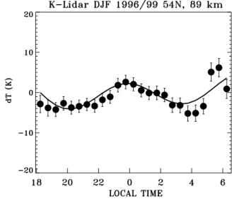
Fig. 1. WINDII temperature semidiurnal and terdiurnal tidal fits
at 55◦N and 89 km height for winter solstice (December, January, and February). The temperature data are two-year composites from 1991 to 1997 fitted simultaneously to 12-h and 8-h tidal harmonics (solid line).
The results from LMS fitting these two-year composites for 1991/93, 1993/95 and 1995/97 seasons with SD and TD tidal harmonics are shown in Fig. 1 and given in Table 1.
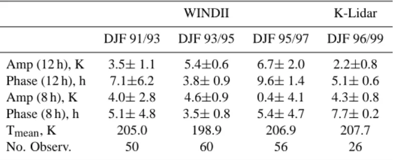
Fig. 2. Potassium lidar temperature semidiurnal and terdiurnal tidal
fits at 54◦N and 89 km height for winter solstice (December, Jan-uary, and February). The temperature data are three-year compos-ites from 1996 to 1999 fitted simultaneously to 12-h and 8-h tidal harmonics (solid line).
From the three DJF data sets considered the 1991/93 data set (Fig. 1a) shows the largest scatter in the dT values which also is reflected in the inferred tidal-fit parameters. The SD and TD amplitudes have about the same magnitude, while the phases have high uncertainty, implying that the phases could be anywhere. Most of the data in the 1991/93 data set come from 1992 (26 days) with a comparable fraction from 1993 (19 days) and very little contribution from 1991 (5 days). The large scatter in dT for LT=12 h–14 h is associated with ob-servations from the first week of January 1992 and could plausibly be a result of stratospheric warming, which was significant in January 1992, in addition to the deterioration of the Rayleigh scattering signal at 89 km. The DJF data for 1993/95 (Fig. 1b) indicate SD and TD tides with compara-ble amplitudes (5.4 K–4.6 K) and practically the same phase (3.8 h–3.5 h), which is very well defined.
The LMS fit to the data from 1995/97 gave an amplitude of 6.7±2 K for the SD tide, while the presence of TD tide was inconclusive due to the large uncertainty in the derived amplitude (0.4±4.1 K) and phase (5.4±4.7 h). The results from the three composite WINDII data sets showed an in-crease in the derived SD amplitudes from 1991 to 1997. The magnitude of the TD tide was of the order of 4 K, except for 1995/97.
Since the potassium lidar temperatures at 54◦N, shown in Fig. 2, employed in the current analysis were obtained from 1996 to 1999, for temporal overlap they are compared with WINDII’s DJF 1995/97 temperature data, shown in Fig. 1c. In a manner similar to WINDII the K-lidar temperatures were fitted both for semidiurnal and terdiurnal tides and the tidal-fit amplitudes and phases at 55◦N are also given in Table 1.
The comparison between the WINDII 1995/97 tempera-ture tidal parameters and the K-lidar 1996/99 data shows that
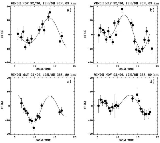
Fig. 3. WINDII temperature semidiurnal and terdiurnal tidal fits at 28◦N (a), (b) and 28◦S (c), (d) for the months of November and May. The temperature data are composites of observations from 1992 to 1996.
the lidar 12-h amplitude of 2.2 K for DJF is a factor of 3 smaller than the WINDII value. However, the phases of the SD tide differ by 4.5 h which might result from the fact that each of the data sets compared samples of only half of the diurnal cycle and thus is biased by the diurnal tide, an effect which at this point cannot be assessed. Further comparison of the WINDII TD tide parameters yielded only a very weak 8-h amplitude with a large uncertainty (0.4±4.1 K) in contrast to the average DJF amplitude of 4.3 K, reported by the K-lidar group. It is interesting that the combined amplitude of the WINDII and K-lidar 12 h+8 h tide is practically the same but with different contributions assigned to the individual har-monics. The WINDII results indicate that globally the 12-h contribution is more dominant compared to that seen by the K-lidar, which could result from the diurnal tide bias, or that the lidar data may include contribution from nonmigrating tides or stationary waves. However, due to the combination of more than one year of observations, the nonmigrating tidal bias is expected to be greatly reduced. The mean background temperatures from WINDII and K-lidar were practically the same, 207 K.
It is not possible to determine the TD tidal contribution based on the WINDII 1995/97 data. In this regard the results are similar to those from 1991/93. The lidar inferred TD amplitude of 4.3 K is in good agreement with the WINDII results. The discrepancy in the 12 h+8 h results is related to a great extent to the individual observations used in these three-month composites. From the 26 nights of observations in the DJF lidar data set, 7 are from December, 12 from Jan-uary and 7 from FebrJan-uary. A review of the WINDII DJF-1995/97 data shows that half of the data for that period are for February (52% from February, 17% from January and 31% December), which could account for the differences ob-served in the fitting of the two DJF data sets. Monthly SD and TD tidal fits for December, January and February indicated a strong TD tide (relative to the SD) in December and January, while in February the SD tidal component was stronger than that for the TD. The results obtained are consistent with these findings.
Table 2a. Temperature tidal-fit parameters at 28◦N and at 89 km height.
No. Obs. Amp (12 h), K Phase (12 h), h Amp (8 h), K Phase (8 h), h Tmean, K
November WINDII 38 7.4±2.5 1.2±0.04 3.8±0.3 6.1±0.9 210.0
K-lidar 12 13.0±0.9 2.4±0.2 7.1±1.5 4.0±0.2 219.5
May WINDII 60 5.4±0.3 9.7±0.4 8.5±1.1 4.2±0.1 199.1
K-lidar 18 7.8±4.3 4.6±1.0 5.8±3.3 7.3±0.6 194.5
Table 2b. WINDII temperature tidal-fit parameters at 28◦S and at 89 km height.
No. Obs. Amp (12 h), K Phase (12 h), h Amp (8 h), K Phase (8 h), h Tmean, K
November 58 2.9±1.0 11.5±3.4 4.5±0.3 5.5±1.1 199.9
May 26 2.5±0.2 4.1±0.1 7.7±0.8 5.6±2.0 199.6
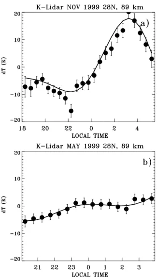
Fig. 4. Potassium lidar temperature semidiurnal and terdiurnal tidal
fits at 28◦N for the months of November (a) and May (b), 1999.
4.2 Subtropical latitudes – 28◦N
WINDII daily zonal mean temperatures were also calculated for the latitude band 23◦N–33◦N centered at 28◦N. As in the mid-latitude case, the mean temperatures for November for each year (1992, 1993, 1995, and 1996) were calculated and subtracted from the zonal daytime means. The observations covered about 11 h of LT (6:00 h to 17:00 h) with gaps of 1 h at 10 h–11 h, and 12 h–13 h, and 2 h between 14 h and 16 h LT. The WINDII amplitude and phases are determined to be 7.4 K and 1.2 h for the SD tides, and 3.8 K and 6.1 h for the TD tide (see Table 2a). The experimental data and the model tidal fits are shown in Fig. 3a and b for 28◦N.
The K-lidar observations at Tenerife (28◦N) for Novem-ber 1999, shown in Fig. 4a, yielded amplitudes of 13 K for the SD tide and 7.1 K for the TD tide which are larger by nearly a factor of 2 than the WINDII values. The phases for the two harmonics are 2.4 h and 4 h, respectively. The phases differ only by about 1 h for the SD harmonic and 2 h for the TD harmonic. As was stated earlier the two data sets sample either daytime or nighttime periods and thus the tidal ampli-tudes and phases derived may be subjected to bias from the diurnal tide. Radar studies of equinoctial phase changes have shown that tides undergo significant and rapid changes from summer to winter conditions as late as the end of November (Tsuda et al., 1988) during which the semidiurnal tidal am-plitudes are significantly reduced. This transition can also be partly responsible for the scatter seen in the WINDII data and the lower zonal mean amplitude compared to the li-dar. The large SD tide amplitudes observed by the K-lidar could also be biased by the presence of nonmigrating tides whose amplitudes have been observed to increase in Octo-ber/November at Tenerife’s latitude and the height where our comparison is made (89 km) (Hecht et al., 1998, Talaat and Lieberman, 1999). We will return to this again in the dis-cussion. For the month of May a composite WINDII tem-perature monthly climatology for the 23◦N–33◦N latitude
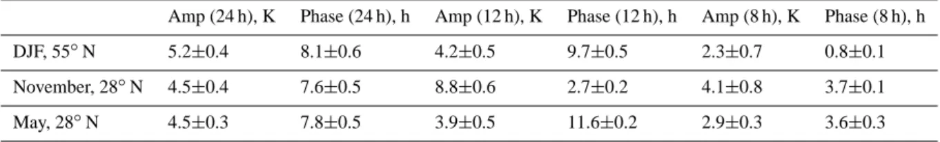
Table 3. Diurnal, semidiurnal and terdiurnal tidal-fit parameters at 89 km height.
Amp (24 h), K Phase (24 h), h Amp (12 h), K Phase (12 h), h Amp (8 h), K Phase (8 h), h
DJF, 55◦N 5.2±0.4 8.1±0.6 4.2±0.5 9.7±0.5 2.3±0.7 0.8±0.1
November, 28◦N 4.5±0.4 7.6±0.5 8.8±0.6 2.7±0.2 4.1±0.8 3.7±0.1
May, 28◦N 4.5±0.3 7.8±0.5 3.9±0.5 11.6±0.2 2.9±0.3 3.6±0.3
band based on observations from 1992, 1993 and 1996 was also created. There are no temperature observations in May 1994, 1995 and 1997 at these latitudes. The composite data set encompasses LT from 5.2 h to 18.5 h with a gap of 2 h between 11:00 LT and 13:00 LT. Adding observations from 1996 to the set did not improve the LT coverage already provided by the 1992/93 observations, but instead reduced the geophysical variability in the data. Fitting the data si-multaneously for 12-h and 8-h oscillations gave amplitudes of 5.4 K and 8.5 K for the SD and TD tides, respectively, while the inferred phases are 9.7 h and 4.2 h, thus indicating a stronger TD tide (see Fig. 3b). The K-lidar tidal parame-ters have amplitudes of the same magnitude as WINDII but in reverse order with a dominant SD tide: 7.8 K for SD and 5.8 K for TD, and phases of 4.6 h and 7.3 h, respectively (see Fig. 4b and Table 2). The amplitudes have large error bars and the WINDII values lie well within. Comparing the tidal results from spring and fall at 28◦N shows that in May both satellite and lidar tidal amplitudes are smaller than those in November with the exception of the WINDII TD tide in May. The WINDII observations also reveal stronger seasonal TD asymmetry (November/May) than that suggested by the lidar observations. Both data sets indicate a warmer mean tem-perature field in November than in May, with a difference of 10 K on a global scale according to WINDII and 25 K from the K-lidar data.
4.3 Seasonal and inter-hemispherical comparisons – 28◦S/28◦N
The global coverage of the satellite observations allows for inter-hemispherical comparisons. For this purpose in the fashion already described daily zonal mean temperatures were also obtained at 23◦S–33◦S, centered at 28◦S for May and November 1992–1996, given in Fig. 3c and d and LMS fitted for semidiurnal and terdiurnal tides. The results ob-tained are given in Table 2b. Having the 28◦S data available allows for two kinds of comparisons: 1) comparison between the November results at 28◦N and those from May at 28◦S, to examine hemispherical variability of the tidal components within the same season, and 2) seasonal variability by com-paring results from May and November at 28◦N and 28◦S.
The LT coverage of the May 28◦S data was similar to that in November at 28◦N, which is to be expected considering the WINDII viewing geometry for the fall season in both hemispheres. This similarity allows for a direct
compari-son of the tidal parameters determined, since in both cases the bias that might be introduced by the LT sampling could be neglected. The November/May comparisons at ±28◦ lat-itude indicate smaller tidal ampllat-itudes with a lesser scatter and smaller standard deviation in the Southern Hemisphere than in the Northern Hemisphere for the same seasons. The inferred amplitudes and phases at 28◦S in May are 2.5 K and 4.1 h for the SD tide, and 7.7 K and 5.6 h for the TD tide, compared to 5.4 K and 9.7 h for SD, and 8.5 K and 4.2 h for TD at 28◦N in November, respectively. In the Southern Hemisphere the TD is stronger than the SD in both months. No seasonal difference is observed in the mean temperatures. Compared to the very few model simulations available, our results at 28◦S are within the amplitude range predicted by GSWM-00 model at 27◦S: 1.8 K (14.4 h) for November and 3 K (16.5 h) for May, although the phases are rather different. 4.4 Diurnal and semidiurnal tide
The relative agreement in the comparison of the tidal param-eters determined from the daytime WINDII observations and the K-lidar nighttime observations encouraged us to carry our tidal analysis one step further by combining the two data sets of residual temperature dT to create a composite dT data set with a full 24-h coverage in LT for the periods of considera-tion (DJF95/97, May and November). These composite data sets were fitted for the D, SD and TD tides and are shown in Fig. 5, while Table 3 gives the tidal-fit parameters resulting from the LMS fitting. Combining the day/nighttime obser-vations allows for an evaluation of the magnitude of the SD tidal parameters determined earlier and assumed to be biased by the diurnal tide. In most cases considered combining the two data sets led to a decrease in the SD and TD tide am-plitudes, as can be expected based on the results reported by Chen et al. (2000) and States and Gardner (2000b).
In the DJF case (Fig. 5a), the amplitude of the SD tide was reduced to 4.2 K compared to the WINDII daytime ob-servations of 6.7 K, while the nighttime SD amplitudes in-creased by a factor of 2. The phase of 9.7 h was identical with the WINDII SD tidal phase of 9.6 h, but larger than the K-lidar value of 5.1 h. The Tenerife SD amplitude in Novem-ber (Fig. 5b) remained the largest of all cases considered, with a magnitude of 8.8 K compared to the WINDII’s 7.4 K and lidar’s 13 K (Table 2a). The phase of 2.7 h is slightly larger than the WINDII SD phase by 1.5 h and is close to the K-lidar result of 2.4 h. Finally, the May case yielded the SD
Table 4. Tidal parameters at 89 km height – self consistent values.
Amp (24 h), K Phase (24 h), h Amp (12 h), K Phase (12 h), h Amp (8 h), K hase (8 h), h Offset, K
JF, 55◦N 6.5±0.3 9.5±0.6 4.1±0.4 10.0±0.2 2.6±0.8 0.7±0.1 −4.3
November, 28◦N 6.5±0.4 9.3±0.7 8.8±0.8 2.7±0.1 3.2±0.4 3.8±0.3 −4.8
May, 28◦N 4.0±0.3 5.8±0.5 4.6± 0.5 11.7±0.2 3.5±0.3 3.7±0.3 +3.9
amplitude of 3.9 K, which is closer to the lidar individual fit-ting (12 h+8 h) result, while it is smaller by a factor of 2 than for WINDII.
The TD tidal contribution to the diurnal temperature varia-tion changed significantly in comparison with the individual fits to the daytime or nighttime observations. For the DJF case the combined data provide a clearly defined TD compo-nent, while the WINDII data alone do not. The phase devi-ates only by 1 h from the lidar nighttime result. In November the amplitude is closer to the WINDII result, while the phase is in better agreement with the K-lidar values. The tidal pa-rameters inferred for May are closer to the WINDII 12h+8h results for that month, as can be seen in Table 3.
Additionally, combining the two data sets leads to the de-termination of the diurnal tidal parameters. Both amplitude and phase of the 24-h tide do not show much variation dur-ing the three observation periods. The 24-h amplitude ranges between 4.5 K and 5.2 K, while the phase is 7.6–8.1 h. The phases are remarkably constant from season to season and at both latitudes, 28◦N and 55◦N. In May at 28◦N there is very little difference in all three tidal harmonics with ampli-tudes of 4.5 K, 3.9 K and 2.9 K, for the D, SD and the TD tide, respectively.
All tidal parameters listed in Table 3 were obtained as-suming that the residuals dT determined from both data sets are deviations from the same background level. As was mentioned earlier, the mean was subtracted to account for the various factors that can lead to differences in the back-ground temperatures (i.e. the different observation periods, zonal coverage, data handling, and individual instrument cal-ibration). It is inevitable that this reduction also removes sys-tematic differences between day and night from the data, i.e. the signature of diurnal tides. Thus, to examine the degree of these possible differences and their effect on the tidal param-eters inferred, the consistency test described in Sect. 3 was applied. The results are shown in Fig. 6 and Table 4. Here the individual data sets are given in open symbols with error bars, while the combined data set after the consistency test is given in solid circles. The consistency test cannot determine the mean background temperature. It gives only a relative offset which might be applied to either of the data sets, as a result of, and consistent with, the harmonic functions fit-ted to them. While for DJF and November the nightly mean is determined to be colder by 4–5 K than the daytime mean at both latitudes, it is calculated to be warmer by a similar amount in May. The consistency corrections affect mostly
the inferred D tidal parameters which may be compared to the results listed in Table 3. The diurnal tide amplitudes and phases for DJF and November are increased by 1.5–2 K and by ∼1.5 h, respectively, while for May the corrections lead to a reduction by ∼2 h in the D phase and a negligible amount in the amplitude. These comparisons show that when complementary observations are available, as in the DJF case (Figs. 5a, 6a), ground-based lidar observations can success-fully be combined with satellite observations to derive diur-nal and semidiurdiur-nal tidal parameters and to study the dynam-ics of the mesopause region. In the other two cases, May and November, the results are also quite encouraging considering the fact that the observation periods (1992/96 for WINDII and 1999 for K-lidar) do not overlap and the possibility for nonmigrating tidal contribution to the K-lidar observations. In November the scatter in the WINDII data is the likely re-sult of both a decrease in the SNR of the lower Rayleigh scattering radiances approaching winter solstice and the geo-physical variability along the 10◦ wide latitude bin, over which the zonal daytime means are obtained. However, the interpretation of the results becomes more complex in view of the possibility that the satellite might be sampling different global longitudinal structures of the tidal modulations, which cannot be seen in the lidar data (Merzlyakov et al., 2001). In addition to improving the determination of the SD tide, com-bining the two data sets also provided information on the di-urnal tidal amplitudes and phases, listed in Table 3 and not previously available from observations at the latitudes con-sidered in this study.
5 Discussion
Fitting the experimental data with 24-h, 12-h and 8-h har-monics at 55◦N and 28◦N gave a good agreement between the regression function and the experimental data. The scat-ter seen in the WINDII temperatures can be attributed at least partly to the fact that the data are composites from three or four (1992/96) years of observations, while the K-lidar re-sults at 28◦N are only for one year 1999, for which there are no correlative WINDII data at present. Year-to-year and geophysical variability along the WINDII 10◦latitude band within which the daily zonal temperatures are determined can be significantly larger compared to the day-to-day variability in a given year and at given location. Such variability has been observed in radar wind semidiurnal tides showing that
Fig. 5. Combined (24 h+12 h+8 h) tidal fit (solid line) to the potassium-lidar nighttime temperatures (solid circles) and the WINDII daytime temperatures (squares) for: (a)
December-February; (b) November, and (c) May.
the phase and amplitude of the semidiurnal tide varies from station to station even in a narrow latitude band of ∼5◦, as was reported by Jacobi et al. (1999).
A great part of what is known about semidiurnal tides at 50◦N–55◦N latitude is from radar wind observations (i.e. Manson et al., 1999; Jacobi et al., 1999), while Na lidar
ob-Fig. 6. Combined (24 h+12 h+8 h) tidal fit (solid line) to the potassium-lidar nighttime temperatures (open circles) and the WINDII daytime temperatures (open squares) after applying the consistency test (the corrected data are in solid circles) for: (a) December-February; (b) November, and (c) May.
servations at mid latitudes, 40◦N–45◦N have provided in-formation on the diurnal variability of the temperature field (i.e. States and Gardner, 1998, 2000a, b; Chen et al., 2000; Williams et al., 1998). Williams et al. (1998) presented esti-mates of the annual nighttime temperature variability based
on Na lidar observations from 1990 to 1997 at Fort Collins, CO, USA (41◦N, 105◦W), which showed that the semidi-urnal tide with a vertical wavelength of 30 km is a dominant tidal perturbation during winter months with an amplitude of 12 K at 90 km height, while Na lidar observations at Urbana, IL, USA (40◦N, 88◦W) yielded SD tidal amplitudes of the order of 5–10 K in the mesopause region (Dao et al., 1995; States and Gardner, 1998). States and Gardner’s (2000b) Na lidar observations of 24-h, 12-h and 8-h tidal amplitudes at 89 km gave a D amplitude of 4.5 K in winter which is weaker by 2 K than the values derived in the present analysis of 6.5 K for DJF at 55◦N after applying the consistency test. There is also a difference of ∼8 h in the phases derived from the two data sets which may arise from the ∼15◦difference in lati-tude. This result is somewhat surprising considering the fact that the D amplitude is expected to peak at ∼40◦N and de-crease in magnitude toward the pole. The amplitudes of 2.6 K derived for the TD tide in DJF are in excellent agreement with the winter Na lidar observations of States and Gard-ner (2000b), while the phases differ by 2h (0.7 h vs. 2.7 h). However, the SD tidal amplitudes are smaller at 55◦N than at 40◦N (4.1 K vs. 7.5 K), with a phase difference of ∼2 h (9.7 h vs. 8 h, Table 2).
The comparison between the Na lidar tidal parameters for spring and fall with the May and November results at 28◦N should consider the classical tidal theory, which predicts that the D has a minimum at ∼25◦N. Indeed, the Na lidar D am-plitudes in spring are larger than our May values (8 K vs. 4 K, respectively), while the fall values are comparable with our November results (7.5 K vs. 6.5 K). There is also very good agreement in SD and TD amplitudes for spring and May, 3.7 K vs. 4.6 K (3.9 K, from Table 3), and 4.6 K vs. 3.5 K, respectively. Finally, our November results indicate a stronger SD tide than that observed in the fall by the Na lidar (8.8 K vs. 2.8 K). The TD amplitudes are of the same magnitude (3.2 K vs. 3 K). Other diurnal lidar measurements at 41◦N by Chen et al. (2000) show no systematic difference at 89 km in spring and fall between daytime and nighttime means, while in winter the night is warmer by ∼6 K that is contrary to our finding. A possible reason for this could be the influence of non-migrating tides on the lidar data.
A large SD amplitude of ∼10 K and phase of 8 h was ob-served at ∼23◦N in October 1993 during the Airborne Lidar and Observations of Hawaiian Airglow (ALOHA-93) cam-paign (Hecht et al., 1995, 1998), in excellent agreement with the SD amplitude derived at Tenerife in November both from WINDII (7.4 K) and the K-lidar (13 K) (Table 2a), and that from the combined 24 h+12 h+8 h tide, 8.8 K (Table 4). The WINDII/K-lidar amplitudes for the D are comparable to the ALOHA-93 values, 6.5 K vs. 7 K, while the WINDII/K-lidar diurnal tide peaks 4 hours later (9.3 h vs. 5.5 h).
Another attempt to combine satellite and ground-based MLT data (Drob et al., 2000) has also led to the derivation of diurnal tide parameters at mid latitudes (41◦N). Com-bining temperature data from Na-lidar, OH rotational tem-peratures and HRDI daytime observations the authors have shown that sampling only half of the diurnal cycle leads
to bias by the diurnal tide manifested in a constant phase at night and a diurnal tidal amplitude of as much as 15 K. The results with bias correction indicated maxima occurring mostly during the day supporting the conclusion by States and Gardner (1998, 2000a, b) and Clancy et al. (1994) that on average mid-latitude temperatures are warmer during day-time at 87 km, similar to our results at 89 km for DJF and November, as shown in Fig. 6. With or without bias correc-tion the estimates of the SD tides were found to be consistent with those of Williams et al. (1998), and States and Gardner (2000b).
Manson et al. (1999) conducted an extensive study on the seasonal and latitudinal variability of diurnal and semidiurnal tides from radar wind observations, including comparisons with the GSWM (Hagan, 1996). It was shown that at 90.5 km height there was a good agreement between the model and observed wind D and SD tidal amplitudes and phases in May and November at subtropical latitudes (∼30◦N) and January at mid latitudes (55◦N), with the May data yielding the best overall agreement between model and wind observations. However, comparisons between the thermal 24-h and 12-h tidal parameters obtained in the current analysis and predic-tions by the GSWM-00 (Hagan et al., 1999), and Forbes-Vial (FV) model (Forbes and Forbes-Vial, 1989) show that the mod-els tend to underestimate the temperature tidal amplitudes, a fact that has been revealed also through comparisons with ground-based Rayleigh and Na lidars (Leblanc et al., 1999; States and Gardner, 2000a, b) and satellite (i.e. Oberheide et al., 2000) temperature data. The average D amplitude for DJF from FV is predicted to be 2 K compared to 6.5 K deter-mined from the experimental data. For November at 28◦N our D amplitude is 6.5 K compared to 3.3 K from FV. The FV amplitude for May is 0.7 K compared to 4 K from the current study. There is no agreement between the modeled and the measured phases.
The diurnal tidal parameters determined in the analysis presented are also compared with the GSWM-00 model pre-diction at 90.5 km height (courtesy of the CEDAR (Coupling, Energetics and Dynamics of Atmospheric Regions) Database and M. Hagan). At 55◦N the amplitude of 1.5 K from the model for January is smaller than our amplitude of 6.5 K, while the phases are opposing (21 h vs. 10 h). In May at 28◦N the model D amplitude and phase of 4.2 K and 5.7 h are in an excellent agreement with the inferred experimental values of 4 K and 5.8 h, respectively. Finally, in November the model diurnal amplitude is smaller by a factor of 2 than the experimental value, 3.1 K vs. 6.5 K, while the phases are about 12 h apart – 23 h (GSWM-00) and 9 h (from the obser-vations).
Several models similar in numerical formulation to the GSWM model of Hagan et al. (1999) have been developed for the assimilation of wind and temperature observations from the HRDI and WINDII experiments on UARS (i.e. Yudin et al., 1997; Khattatov et al., 1997). The satellite wind data were used to evaluate tidal dissipation among other pa-rameters, which is poorly represented in the earlier versions of the GSWM model. Day/nighttime wind observations from
WINDII in the 90–110 km height range and daytime winds from HRDI below 90 km were employed in the tuned mech-anistic tidal model (TMTM) (Yudin et al., 1997), in order to model diurnal and semidiurnal tidal parameters (amplitude and phase) for winds and temperatures in the height range of 85–110 km and ± 40◦latitude around the equator for March and January. The TMTM simulations gave a D amplitude of ∼8 K at 28◦N and 89 km height for March 1993, which is about a factor of 2 higher than the amplitude for May derived in the current analysis.
The seasonal behavior of the diurnal tide was also com-puted from the HRDI/UARS data (Khattatov et al., 1997). Meridional diurnal tidal winds derived from the HRDI data were used in the linearized tidal equations to solve for the diurnal tidal oscillations in the zonal and vertical velocity, pressure, temperature and dissipation in the MLT region pro-ducing monthly mean latitude/altitude cross sections of tidal wind and temperature fields at ±40◦ latitude around the equator for the combined 1992/1993 year. The 24-h tidal amplitudes at 89 km and at 28◦N are predicted to be less than 5 K for May, while the November value is slightly above 5 K in very good agreement with results from this study of 4 K and 6.5 K for May and November, respectively. Another model simulation with the Spectral Mesosphere/Lower Ther-mosphere Model (SMLTM) by Akmaev et al. (1997) of the diurnal tide for equinox and solstice conditions indicated an amplitude of ∼8 K at 89 km for April compared to the 4 K for May from the WINDII/K-lidar analysis and phase of ∼11 h compared to 5.8 h.
The seasonal variability of the diurnal tide was also stud-ied using the Canadian middle atmosphere general circula-tion model (CMAM). Employing 2-year model simulacircula-tions McLandress (1997) showed that the diurnal temperature am-plitude, which is largest near the equator at 90 km, exhibits strong semiannual variations at low latitudes in the meso-sphere ranging from 20 K at equinox to 7 K at solstice in good agreement with the Yudin et al. (1997) results. The CMAM amplitude of the thermal diurnal tide at 28◦N in November is 3.3 K compared to the inferred amplitude of 6.5 K, while in May the model predicts a D-tide amplitude of 5.6 K, compared to 4 K from this study. The comparison shows that there is very good agreement for spring equinox between the CMAM and the inferred 24-h amplitude from the combined satellite/lidar observations, while in the fall the observed diurnal amplitude is a factor of 2 larger than the model predictions.
Finally, we need to address the possibility that the tidal parameters inferred might be biased by the effect of nonmi-grating tides, particularly at Tenerife, which have not been removed from the lidar data. However, the agreement in the results from the separately fitted WINDII and K-lidar data sets suggested that the nonmigrating tidal bias might not be significant. In view of the results reported by Hagan and Forbes (2002) it is reasonable to assume a high year-to-year variability in the tropospheric latent heat source and the prop-agation conditions affecting the magnitude and phasing of the nonmigrating tide. The assumption made in our
analy-sis that the nonmigrating tidal bias is insignificant is reason-able at 55◦N, as the data employed are averaged over sev-eral years and months (1996–1999, and DJF), thus partially averaging-out the nonmigrating tidal contribution. This is not necessarily so for the lidar data from Tenerife, as they are only from one year/month of observations (November/May, 1999). The analysis of nonmigrating tide signatures in HRDI mesospheric and lower thermospheric winds and tempera-tures revealed a prominent equatorial feature associated with nonmigrating tides at about 85–92 km height during Octo-ber/November with an amplitude of about 4 K (Hecht et al., 1998; Talaat and Lieberman, 1999). Results of comparable magnitude were also reported at 20◦N by Hecht et al. (1998). Thus, the large SD tidal amplitude of 13 K inferred from the lidar data in November can still include a nonmigrating tidal component, while still being in an agreement with WINDII and other ground-based and model results.
Apart from the HRDI results most of the thermal non-migrating tidal studies concern predictions by general cir-culation models (GCM). For example, at 86 km height the DNM-RAS GCM (e.g. Grieger et al., 2002; N. Grieger, personal communication, 2003) gives amplitudes of 1.3
±2.1 K, 0.7±1.2 K and 1.1±0.6 K for the 24-h, 12-h, and 8-h nonmigrating components, respectively, for November and 2.4±1.3 K, 0.8±0.7 K and 0.7±0.5 K for May at 28◦N. For January at 56◦N the GCM nonmigrating tidal amplitudes are below the rms variance, 0.2 K, 0.3 K, and 0.2 K for the 24-h, 12-h, and 8-h harmonics, respectively. The GSWM also es-timates the nonmigrating tidal amplitudes to be below 1 K at the latitudes considered in the current study.
It is intriguing to see that the magnitude of the “offset” determined in the self-consistent test (Table 4) is compara-ble with the nonmigrating tidal amplitude inferred from the HRDI data (Hecht et al., 1998; Talaat and Lieberman, 1999). However, the available data and the data handling approach employed in the current study do not permit further exami-nation of this possibility.
6 Summary
The results obtained can be summarized as follows:
1. WINDII daily zonal mean temperatures and K-lidar nightly temperature variations were employed to infer tidal parameters at 89 km height. The analysis concen-trated on the winter solstice period from December to February at 55◦N and the end of spring and fall equinox periods, in May and November at 28◦N.
2. Due to their limited local time coverage only semidi-urnal and terdisemidi-urnal tidal parameters could be derived from each of the data sets. The results obtained showed satisfactory agreement considering the differences in the observation periods, data acquisition and diurnal tide bias.
3. Even after the removal of the mean temperatures the WINDII data for DJF revealed variability in the
two-year composite SD amplitudes, as the latter in-creased over the 6 year period considered. The TD am-plitudes did not vary, although the inferred phases had a significant uncertainty. In terms of the hemispherical variability the SD amplitudes in May and November at 28◦N were stronger than those inferred from the zonal daily means at 28◦S by a factor of ∼2. The inferred TD amplitudes and phases were very similar in magni-tude between both hemispheres. The results obtained suggest that although the TD tide is present most of the observed tidal variability is due to variability in the D and SD tidal components.
4. The agreement in the SD- and TD-tide parameters in-ferred allowed the two data sets to be combined in order to retrieve the diurnal, semidiurnal and terdiurnal tidal parameters. The DJF results show a dominant diurnal tide with an amplitude of 6.5 K and phase of 9.5 h at 55◦N, with a SD tide second in strength with an am-plitude of 4.1 K and phase of 10 h. In November, the SD tide at 28◦N was the strongest with 8.8 K ampli-tude, compared to 6.5 K of the D tide. It is notable that according to our observations the diurnal tide amplitude and phase at 28◦N and 55◦N at 89 km height appear the same for November and DJF. In May the semidiurnal tide amplitude is comparable with the diurnal tide, but about a factor of 2 smaller than the November values. There is a very good agreement in the inferred terdiur-nal parameters for November and May.
5. The results obtained are in various degrees of agreement with GSWM-00, CMAM and other tidal models in pre-dicting the diurnal tide in May, but in general the in-ferred tidal amplitudes are a factor of 2 to 4 larger than the models. Yet much better agreement was obtained with other ground-based experimental data.
6. These comparisons show that when complimentary ob-servations are available ground-based lidar obob-servations can successfully be combined with satellite observa-tions to derive diurnal and semidiurnal tidal parameters and study the dynamics of the mesopause region. Acknowledgements. The authors thank U. von Zahn for his kind guidance, advice and helpful discussion during the course of this study. We thank N. Grieger for his comments and useful discus-sion. One of the authors (MGS) would like to acknowledge the support by the Leibniz-Institute for Atmospheric Physics and the Optical Sounding Group received during her visit and work on this project. We also thank Y. J. Rochon and B. H. Solheim for provid-ing the WINDII Level 2 data. We are grateful for the support of the Instituto de Astrofisica de Canarias and the Kiepenheuer Institut f¨ur Sonnenphysik during the lidar operation at Tenerife. Funding for a part of this research was provided by a Natural Science and Engi-neering Research Council of Canada (NSERC) Research Grant.
Topical Editor U.-P. Hoppe thanks two referees for their help in evaluating this paper.
References
Akmaev, R. A., Yudin, V. A., Ortland, D. A.: SMLTL simulations of the diurnal tide: comparison with UARS observations, Ann. Geophys. 15, 1187–1197, 1997.
Beagley, S. R., de Grandpre, J., Koshyk, J. N., McFarlane, N. A., and Shepherd, T. G.: Radiative-dynamical climatology of the first-generation Canadian Middle Atmosphere Model, Atmosphere-Ocean, 35, 293–331, 1997.
Berger, U.: Numerische Simulation klimatolgischer Prozesse und thermischer Gezeiten in der mittlere Atmosph¨are, Mitteil. Inst. Met. Klimatol., K¨oln, 191, 1994.
Berger, U. and U. von Zahn: The two-level structure of the mesopause: A model study, J. Geophys. Res., 104, 22 083– 22 093, 1999.
Burrage, M. D., Wu, D. L., Skinner, W. R., Ortland, D. A., and Hays, P. B.: Latitude and seasonal dependence of the semidi-urnal tides observed by the high-resolution Doppler imager, J. Geophys. Res., 100, 11 313–11 321, 1995a.
Burrage, M. D., Hagan, M. E., Skinner, W. R., Wu, D. L., and Hays, P. B.: Long-term variability in the solar diurnal tide observed by HRDI and simulated by the GSWM, Geophys. Res. Lett, 22, 2641–2644, 1995b.
Chapman, S. and Lindzen, R. S.: Atmospheric Tides, D. Reidel, Norwell, Mass., 1970.
Chen, H. M., White, A., Krueger, D. A., and She, C. Y.: Daytime mesopause temperature measurements with a sodium-vapor dis-persive faraday filter in a lidar receiver, Opt. Lett., 21, 1093–095, 1996.
Chen, S., Hu, Z., White, M. A., Chen, H., Krueger, D. A., and She, C. Y.: Lidar observations of seasonal variations of diurnal mean temperature in the mesopause region over Fort Collins, Colorado (41◦N, 105◦W), J. Geophys. Res., 105, 12 371–12 379, 2000. Clancy, R. T., Rusch, D. W., and Callan, M. T.: Temperature
min-ima in the average thermal structure of the middle atmosphere (70–80) from analysis of 40–92 km SME global temperature pro-files, J. Geophys. Res., 99, 20 533–20 544, 1994.
Clemesha, B. R., Simonich, D. M., Batista, P. P., and Kirchhoff, V. W. J. H.: The diurnal variation of atmospheric sodium, J. Geo-phys. Res., 87, 181–186, 1982.
Crary, D. J. and Forbes, J. M.: On the extraction of tidal information from measurements covering a fraction of a day, Geophys. Res. Lett, 10, 580–582, 1983.
Dao, P. D., Farley, R., Tao, X., and Gardner, C. S.: Lidar obser-vations of the temperature profile between 25 and 103 km: Evi-dence of strong tidal perturbation, Geophys. Res. Lett., 22, 2825– 2828, 1995.
Drob, D. P., Picone, J. M., Eckermann, D., She, C. Y., Kafkalidis, J. F., Ortland, D. A., Niciejawski, R. J., and Killeen, T.: Mid-latitude temperatures at 887 km: Results from multi-instrument Fourier analysis, Geophys. Res. Lett., 27, 2109–2112, 2000. Dudhia, A., S.E. Smith, A.R. Wood, and F.W. Taylor, Diurnal and
semi-diurnal temperature variability of the middle atmosphere, as observed by ISAMS, Geophys. Res. Lett., 20, 1251-1254, 1993.
Fesen, C. G., Roble, R. G., Ridley, E. C.: Thermospheric tides at equinox-simulations with coupled composition and auroral forc-ing, 1. Diurnal component, J. Geophys. Res., 96, 3647–3661, 1991.
Forbes, J. M. and Vial, F.: Monthly simulations of the semidiurnal tide in the mesosphere and lower thermosphere, J. Atm. Terr. Phys., 51, 649–661, 1989.
Forbes, J. M., Manson, A. H., Vincent, R. A., et al.: Semidiurnal tide in the 80–150 km region: an assimilative data analysis, J. Atmos. Terr. Phys., 56, 1237–1249, 1994.
Forbes, J. M., Kilpatrick, M., Fritts, D., Manson, A. M., Vincent, R. A.: Zonal mean and tidal dynamics from space: an empirical examination of aliasing and sampling issues, Ann. Geophysicae, 15, 1158–1164, 1997.
Fricke-Begemann, C., H¨offner, J., von Zahn, U.: The potassium density and temperature structure in the mesopause region (80– 100 km) at a low latitude (28◦N), Geophys. Res. Lett., 29, 2067, doi:10.1029/2002GL015578, 2002a.
Fricke-Begemann, C., Alpers, M., and H¨offner, J.: Daylight rejec-tion with a new receiver for potassium resonance temperature lidars, Opt. Lett., 27, 1932–1934, 2002b.
Geller, M. A., Yudin, V. A., Khattatov, B. V., Hagan, M. E.: Mod-eling the diurnal tide with dissipation derived from UARS/HRDI measurements, Ann. Geophysicae, 15, 1198–1204, 1997. Gille, S. T., Hauchgecorne, A., and Chanin, M. L.: Semidiurnal
and diurnal tidal effects in the middle atmosphere, as seen by Rayleigh lidar, J. Geophys. Res., 96, 7579–7587, 1991. Grieger, N., Volodin, E. M., Schmitz, G., Hoffmann, P., Manson,
A. H., Fritts, D. C., Igarashi, K., Singer, W.: General circulation model results on migrating and nonmigrarion tides in the meso-sphere and lower thermomeso-sphere, Part I: comparison with obser-vations, J. Atmos. Solar-Terr. Phys., 64, 897–911, 2002. Hagan, M. E.: Comparative effects of migrating solar sources on
tidal signatures in the middle and upper atmosphere, J. Geophys. Res., 101, 21 213–21 222, 1996.
Hagan, M. E. and Forbes, J. M.: Migrating and nonmigrating diur-nal tides in the middle and upper atmosphere excited by tropo-spheric latent heat release, J. Geophys. Res., 107 (D24), 4754, doi:10.1029/2001JD001236, 2002.
Hagan, M. E., Burrage, M. D., Forbes, J. M., Hackney, J., Randel, W. J., Zhang, X.: GSWM-98: Results of migrating solar tides, J. Geophys. Res., 104, 6813–6828, 1999.
Hays, P. B., Abreu, V. J., Dobbs, M. E., et al.: The High resolution Doppler imager on the Upper Atmosphere Research Satellite, J. Geophys. Res., 98, 10 713–10 723, 1993.
Hecht, J. H., Ramsay Howat, S. K., Walterscheid, R. L., Isler, J. R.: Observations of variations in airglow during ALOHA-93, Geo-phys. Res. Lett., 22, 2817–2820, 1995.
Hecht, J. H., Walterscheid, R. L., Roble, R. G., Lieberman, R. S., Talaat, E. R., Ramsay Howat, S. K., Lowe, R. P., Turnbull, D. N., Gardner, C. S., States, R., and Dao, P. D.: A comparison of atmo-spheric tides inferred from observations at the mesopause during ALOHA-93 with the model predictions of the TIME-GCM, J. Geophys. Res., 103, 6307–6321, 1998.
Hedin, A. E.: Extension of the MSIS thermospheric model into the middle atmosphere, J. Geophys. Res., 96, 1159–1172, 1991. Hitchman, M. H. and Leovy, C. B.: Diurnal tide in the equatorial
middle atmosphere as seen in LIMS temperatures, J. Atmos. Sci., 42, 557–561, 1985.
Jacobi, Ch., Portnyagin, Yu., Solovjova, T. V., et al.: Climatology of the semidiurnal tide at 52◦–56◦N from ground-based radar wind measurements 1985–1995, J. Atmosph. Solar-Terr. Phys., 61, 975–991, 1999.
Keckhut, P., Gelman, M. E., Wild, J. D., et al.: Semidiurnal and diurnal temperature tides (30–55 km): Climatology and effect on UARS-LIDAR data comparisons, J. Geophys. Res., 101, 10 299– 10 310, 1996.
Khattatov, B. V., Geller, M. A., Yuding, V. A., and Hays, P. B.: Diurnal migrating tides as seen by the high-resolution Doppler
imager/UARS: 2 Monthly mean global zonal and vertical veloci-ties, pressure, temperature, and inferred dissipation, J. Geophys. Res., 102, 4423–4435, 1997.
Leblanc, T., McDermit, I. S., Ortland, D. A.: Lidar observations of the middle atmospheric thermal tides and comparison with the High Resolution Doppler Imager and Global-Scale Wave model: 1. Methodology and winter observations at Table moun-tain (34.4◦N), J. Geophys. Res., 104, 11917–11929, 1999. Manson, A. H. and Meek, C. E.: Middle atmosphere (60–110 km)
tidal oscillations at Saskatoon, Canada (52◦N, 107◦W) during 1983–1984, Radio Science, 20, 1411–1451, 1985.
Manson, A. H., Meek, C. E., Kurschener, D., Teitelbaum, H., Schneider, R., Smith, M. J., Fraser, G. J., Clark, R. R.: Climatol-ogy of semi-diurnal and diurnal tides in the middle atmosphere (70–110 km) at middle latitudes, J. Atmos. Terr. Phys. 51, 579– 593, 1989a.
Manson, A. H., Meek, C. E., Kurschener, D., Teitelbaum, H., Schneider, R., Smith, M. J., Fraser, G. J., Clark, R. R.: Global behaviour of the height/seasonal structure of tides between 40◦ and 60◦latitudes, Handbook for MAP, 27, 303–316, 1989b. Manson, A., Meek, C., Hagan, M., et al.: Seasonal variations of the
semi-diurnal and diurnal tides in the MLT: multi-year MF radar observations from 2 to 70◦N, and the GSWM tidal model, J. Atmos. Solar-Terr. Phys., 61, 809–828, 1999.
McLandress, C.: Seasonal variability of the diurnal tide: Results from the Canadian middle atmosphere general circulation model, J. Geophys. Res., 102, 29 747–29 764, 1997.
McLandress, C., Shepherd, G. G., and Solheim, B. H.: Satellite ob-servations of thermospheric tides: results from the Wind Imag-ing Interferometer on UARS, J. Geophys. Res., 101, 4093–4114, 1996.
Meriwether, J., Gao, X., Wickwar, V., Wilkenson, T., Beissner, K., Collins, S., and Hagan, M.: Observed coupling of the meso-spheric inversion layer to the thermal tidal structure, Geophys. Res. Lett., 25, 1479–1482, 1998.
Merzlyakov, E. G., Portnyagin, Y. I., Jacobi, Ch., et al.: On the longitude structure of the transient day-to-day variation of the semidiurnal tide in the mi-latitude lower thermosphere: – I. Win-ter Season, Ann. Geophys. 19, 545–562, 2001.
Oberheide, J., Hagan, M. E., Ward, W. E., Riese, M., Offermann, D.: Modeling the diurnal tide for the Cryogenic Infrared Spec-trometers and telescope for the Atmosphere (CRISTA) 1 time period, J. Geophys. Res., 105, 24 917–24 929, 2000.
Offermann, D., Grossmann, K.-U., Barthol, P., Knieling, P., Riese, M., and Trant, R.: The Cryogenic Infrared Spectrometers and Telescopes for the Atmosphere (CRISTA) experiment and mid-dle atmosphere variability, J. Geophys. Res., 104, 16 311–16 325, 1999.
Oldag, J.: Gezeiteneffecte in der Mesopausenregion aus Lidar-beobachtungen ¨uber K¨uhlungsborn und Teneriffa, PhD Thesis, Univ. of Rostock, 2001.
Pancheva, D. and Mukhtarov, P.: Variability of mesospheric dy-namics observed at Yambol (42.5◦N, 26.6◦E) by meteor radar, J. Atmos. Terr. Phys., 56, 1271–1278, 1994.
Pendleton Jr., W. R., Taylor, M. J., and Gardner, C. S.: Terdiurnal oscillations in OH Meinel rotational temperatures for fall con-ditions at northern mid-latitude sites, Geophys. Res. Lett., 27, 1799–1802, 2000.
Reber, C. A., Trevathan, C. E., McNeal, R. J., and Luther, M. R.: The Upper Atmosphere Research Satellite (UARS) Mission, J. Geophys. Res., 98, 10/,643–10 647, 1993.