Revised January 1983 LIDS-P-1149-A
A DISTRIBUTED ALGORITHM FOR MINIMUM WEIGHT DIRECTED SPANNING TREESt
Pierre A. Humblet*
28 January 1983
*The author is with the department of Electrical Engineering and Computer Science, and the Laboratory for Information and Decision systems,
Massachusetts Institute of Technology, Cambridge MA 02139. Phone (617)
253-7250.
tThis research was conducted at the M.I.T. Laboratory for Information and Decision Systems with partial support provided by the Defense Advanced Projects Agency under Contract ONR-N00014-75-C-1183 and the National Science Foundation under Contract NSF-ECS 79-19880.
Abstract
A distributed algorithm is presented for constructing minimum weight directed spanning trees (arborescences), each with a distinct root node, in a strongly connected directed graph. A processor exists at each node. Given the weights and origins of the edges incoming to their nodes, the processors follow the algorithm and exchange messages with their neighbors until all arborescences are constructed. The amount of
2.
information exchanged and the time to completion are O(INjl).1. Introduction
Having trees with edges directed away from their roots is useful in communication networks when one wishes to broadcast information from a node to other nodes in the network. Trees with edges directed toward the root have been proposed for use in distributed database systems [102. When the topology of the network changes owing to failures or additions of links or nodes, it is desirable to be able to build the trees in a distributed manner, without having to rely on a central node that can be inaccessible. Dalal [5] and Dalal and Metcalfe [4] have described a number of distributed algorithms to construct directed spanning trees
(arborescences).
If there is a cost (or weight) associated with the use of a link in the network, it is useful to determine minimum weight directed trees. This is the object of this paper, where we describe a distributed algorithm to build minimum weight arborescences, one rooted at each node of the network.
2
More precisely, we consider a strongly connected directed graph consisting of a finite set N of nodes and a set E C NxN of edges with a finite weight assigned to each edge e. We assume that the nodes have distinct identities that are ordered. The edge from node i to node j is said to be outgoing from i, incoming to j, and adjacent to i and j. Initially a processor located at a node is given the node identity and the weights and origins of all edges incoming to the node . Each processor performs the same local algorithm, which consists of sending messages over adjacent edges, waiting for incoming messages and processing them. Messages can be transmitted independently in both directions on a directed edge, and arrive after an unpredictable but finite delay, without error and in sequence (this can be achieved by link level protocols that are not described here).
After a node completes its local algorithm, it knows which adjacent edges are part of a minimum weight directed spanning tree (arborescence) rooted at each node.
An interesting result, besides the algorithm itself, is that the amount of communication between the nodes to find the INI optimal arborescences (I I denotes set cardinality) is O(INI[), which is the same order of magnitude as what it takes to construct any INI arborescences. The time to complete the algorithm is also O(INI12).
If the network graph is not directed, then the problem simplifies to finding a minimum weight spanning tree. Distributed algorithms to that effect have been given by Dalal [5], Spira [11] and Gallager, Humblet. and
Spira
[8].
The next section of the paper contains a review of the centralized algorithm to find minimum weight arborescences. It is then explained how the functions can be distributed. The communication cost and running time analysis follow. A precise description of the distributed algorithm appears in the Appendix.
2. Review of minimum weight arborescences
We assume the reader is familiar with the elementary definitions and properties of graphs, paths, cycles, trees, etc. which can be found for example in [9]. In particular a graph is strongly connected if for every pair of nodes there is a directed path with the first node as origin and the second as destination. An arborescence rooted at a node is a directed tree such that one edge in the tree is incoming to each node, except the root (the choice of "incoming to" is arbitrary). The weight of an arborescence is the sum of the weights of the edges it includes.
Our objective is to find INI minimum weight arborescences, one rooted at each node. This is possible if and only if the graph is strongly connected. A centralized algorithm to that effect has first been described by Chu and Liu [3], and rediscovered by others [6] , [1] using different methods. Tarjan [12] gives an efficient implementation (see also [2]). The algorithm is also described in [9]. -We review it briefly
in this section. It rests on four observations:
and only one edge incoming to every other node. Thus if a constant is added to the weights of all edges incoming to a node, the weights of the arborescences change by the same amount and minimum weight arborescences before the change remain so after the change. Thus we can, and from now on will, assume that at least one edge incoming to each node has zero weight, and that the other edges have non negative weights.
2) There exists a directed cycle of zero weight edges, as a traveller starting at any node and walking in reverse direction on zero weight edges will always be able to do so, and will eventually visit the same
node twice, the graph being finite.
3) If a set Le of zero weight edges form a directed cycle, with Ln denoting the set of nodes in the cycle, then for any node r there is a minimum weight arborescence rooted at r such that all edges in Le, except one, are in the arborescence. The edges in the arborescence but not in Le form a minimum weight arborescence for the reduced graph obtained by merging all nodes in Ln into a single node; if r is in Ln, the new arborescence is rooted at this new node instead of at r.
This observation is proved (figure 1) by:
starting with any optimal arborescence rooted at r,
finding the first node f in Ln on a directed path (in the arborescence) from r to any node n in Ln,
removing from the arborescence all edges incoming to nodes in Ln\{f} (\ denotes set subtraction),
and adding all edges in Le, except the one incoming to f
paragraph above. It is optimal as all added edges have zero weight, and all removed edges have non negative weight. The edges in the arborescence but not in Le form an arborescence for the reduced graph, with same weight as the original arborescence. If the smaller arborescence had not minimum weight, the original arborescence would not either.
4) The edges in Le that belong to the new arborescence rooted at f also belong to the new arborescence rooted at r.
These four observations suggest the following recursive algorithm to find minimum weight arborescences.
For each node, add a constant to the weights of the incoming edges, so that their minimum weight becomes zero.
Select enough zero weight edges to form a directed cycle (its existence is guaranteed by observation 2).
Let Le and Ln be the sets of edges and nodes in the cycle. For every edge e in Le, incoming to node f(e) say, mark e as
being on the arborescences rooted at the nodes in Lnjf(e)}.
By observation 3), the other edges of the arborescences can be determined recursively by considering the reduced graph obtained by
replacing all nodes in Ln by a single node (called a cluster).
The general step of the algorithm is as follows.
Start with a graph whose nodes are clusters of nodes, with optimal arborescences defined inside each cluster.
For each cluster subtract a constant. from the weights of the edges incoming to the cluster from nodes outside, so that their minimum weight becomes zero.
Select enough zero weight edges to form a directed cycle of clusters.
Let Le and Lc be the sets of edges and clusters in the cycle. For each edge e in Le, incoming to node f(e) in cluster c(e)
marked as belonging to the arborescence rooted at f(e) as belonging also to the arborescences rooted at all nodes
included in clusters in Lc\{c(e)}, thus exploiting observation 4).
Replace all nodes included in clusters in Lc by a single cluster and repeat the procedure until only one cluster remains.
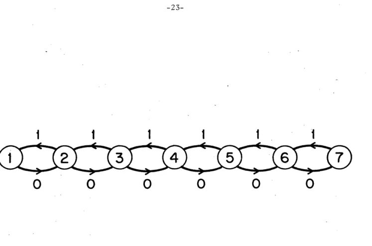
Note that NRG, the number of reduced graphs produced by the algorithm, lies between one and INI-1. The upper bound results from the fact that a cycle Le will give rise to a reduced graph with ILejl- >4 1 fewer nodes; the bound can be achieved if all cycles contain two edges (e.g figure 2). The total number of edges that ever become part of a cycle is equal to INI + NRG - 1, as one incoming edge is selected for every node and every cluster, except the last one.
A naive implementation of the algorithm-requires O(JEJINI) operations. This can be reduced to O(IEI log INt +
INIV)
, or O(INI*) for dense graphs, by making use of special data structures [12] that speed up the determination of a minimum weight incoming edge. Surprisingly, no way is known to significantly simplify the logic of the algorithm if only the minimum weight arborescence rooted at a single given node is desired.1 1
The term JINIJ does not appear in [12] because only one maximum weight arborescence is sought there
7
3. Description of the distributed algorithm
A precise description of the distributed algorithm appears in Appendix A. It has been implemented in a simulation program and found to work correctly. We sketch here how the main functions of the centralized algorithm, i.e. detection of cycles, updating of the arborescences and selection of a minimum weight cluster incoming edge can be distributed. We first describe the data structure maintained by the nodes.
As in the centralized algorithm, each node is part of a cluster, which initially contains only the node itself. A node knows to which node in the cluster (the Cluster_stem) the minimum weight cluster incoming edge is incoming. It also knows the identity of the cluster (Cluster_lID), defined as the largest node identity in the cluster.
In the course of the algorithm edges will be selected. The set of all nodes that have a directed path of selected edges to a given node is called the Known set of that node. A node will also decide that some of its adjacent edges belong to minimum weight arborescences. Inc edgeEn] denotes the incoming edge belonging to the arborescence rooted at node n, while Out_edge_set[n] denotes the set of outgoing edges belonging to that
arborescence.
All nodes are initially considered to be asleep. In response to a command from a higher level procedure with which'we are not concerned here a number of nodes can wake up; they in turn awaken the other nodes by sending messages, so that eventually all nodes will be awake. A node waking up initializes the Known_set as containing only itself and sets
8
itself as Cluster_stem, selects a minimum weight incident edge (called the Stem_edge) and sends the message CONNECT({Node_ ID}) on that edge.
We know the set of Stem_edges contains at least one cycle that we wish to detect. This can be done by having each node send back its identity (in a message LIST({Node_iD})) on the edges on which CONNECT was received, adding to Knownset those identities that it receives, and forwarding an identity the first time it is received. Note that all nodes in a cycle will receive their own identity (that has gone around the cycle). They will not receive any identity from nodes outside the cycle (each node in the cycle has only one Stem_edge, outgoing from another node in the cycle), and, because the ordering of messages sent on a link is preserved, will not receive any identities after having received their own. So at the end of this phase all nodes that are in a cycle know it, and have Known set equal to the identities of the other nodes in the cycle.
Our algorithm follows this outline, with small modifications: when a node receives a CONNECT(Set) message on edge 1, it also sets the variable Neighbor_setEl] to Set. When a node receives a node identity in a LIST message that also appears in Neighbor_set[l], it has detected a cycle, knows that edge 1 belongs to the cycle and also knows the identity of the node 1 is incoming to; that identity is not forwarded on edge 1.
With these modifications, if node identity n is included in a LIST message transmitted on an edge e, then e is in the cycle but is not incoming to n, therefore e is part of the arborescence rooted at n. Thus
the Inc_edge's and Out_edge_set's can be updated as LIST messages are received and transmitted.
Now that a cycle, and thus a new cluster, is identified the nodes must collaborate to find a minimum weight cluster incoming edge, incoming to
the new Cluster stem. We will show later how this can be done. The new Cluster_stem then sends CONNECT(Knownset) on its new Stem_edge, while the other nodes set their Stem edge's to their incoming edges on the arborescence rooted at the Cluster stem
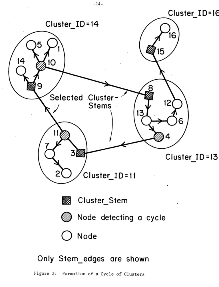
We now explain how to detect cycles of clusters of nodes (figure 3). A node receiving CONNECT(Set) on edge 1 sets Neighbor_set[El to set and answers with LIST(Knownset). The neighboring Clusterstem receives the LIST(Set) message and forwards it on its arborescence , throughout its cluster and beyond on edges on which CONNECT has been received. The criterion for detecting the existence of a cycle is that Set and Neighbor set(l) are not disjoint for some edge 1 outgoing from the cluster.
The detection of a cycle is thus always done at a neighbor of a Cluster_stem (with the neighbor not a part of the same cluster). When this occurs the neighbor sends a CYCLE message to the Clusterstem which retransmits it on its arborescence throughout its cluster, but not outside, contrary to the LIST messages. Thus CYCLE messages are only retransmitted on edges belonging to Internal set, i.e. the set of edges joining two nodes in the same cluster.
10
Note that many cycles can be formed concurrently, but that at a given time a node can only participate in the formation of a single cycle, as it has selected a single Stem_edge. For example in figure 4 the cycles {1,2,3,4} and {5,6,7} can be formed simultaneously, but the bigger cycle
{8,{1,2,3,4},9,{5,6,7},10}
can only be formed after the two smaller cycles.The updating of Inc_edge's and Out_edge_set's can still be done as explained above, as a node identity is never forwarded in a LIST message sent to its own cluster.
The determination of the minimum weight cluster incoming edge can be done easily by taking advantages of the tree structures that are built. Observe (figure 3) that the set of Stem_edges in a cluster, minus the Stem_edge of the Cluster_stem of a "selected" component cluster, form an arborescence rooted at that Cluster stem. We choose as selected cluster the one with largest Cluster_ ID.
When triggered by the reception of a CYCLE message, all nodes collaborate to find the minimum weight cluster incoming edge. Starting with the leaf nodes, they send on the selected arborescence the message REPORT(Bestnode,Best_weight), where Best_weight is the weight of the minimum weight cluster incoming node they know about, incoming to Best_node. To maintain order in the propagation of the REPORT message
toward the selected Cluster stem, a node cannot send it before it has received a CYCLE message on its Stem edge, and REPORT messages from all its descendants in the arborescence. This is implemented by initially
setting a variable Wait count to 1, incrementing it when a CYCLE message is sent (except if to the selected Cluster_stem), and decrementing it when a CYCLE or REPORT message is received, until it reaches O.
Eventually the selected Clusterstem will find the new Cluster stem and broadcast a message UPDATE(New_cluster_stem,Best_weight) to all nodes in
the cluster. All nodes subtract Best weight from the weights of their incoming edges, while New_clusterstem also sends CONNECT(Knownset) on its Stemedge, as explained above. We choose to do the broadcasting of the UPDATE message on the arborescence rooted at Newclusterstem, thus insuring that a LIST message sent by New clusterstem does not reach a node before the UPDATE message has reached that node.
The algorithm terminates when the weight carried in the UPDATE message is Qo , indicating that there are no more cluster incoming edges.
We do not go through the tedious exercise of giving a formal proof of correctness. It would involve showing that the distributed algorithm selects the same edges as the centralized algorithm does (if they use the same tie breaking rule), and detects the same cycles. We would also prove the correctness of the procedure to collect information at the selected Cluster_stem and to disseminate the result throughout the cluster.
12
4. Communication and computation costs analysis
In this section we compute the amounts of communication and computation that take place between and in the nodes during the course of the algorithm, and we compare them with those of other algorithms. Starting with communication cost, note that the messages CYCLE, REPORT and UPDATE have constant lengths, while the messages CONNECT and LIST have variable lengths, as they include a Set. We will first evaluate the amount of information carried in these two messages.
Every time a node identity is included in a LIST message transmitted on an edge, the edge becomes part of the corresponding arborescence. Thus the total number of node identities transmitted in LIST messages is INI!? - INI, and this is also an upper bound on the number of LIST messages.
A node identity is also transmitted in CONNECT messages only on edges that are part of a cycle, but not part of the corresponding arborescence. As seen above, the number of such edges is precisely NRG (between 1 and INI-1), thus the total number of node identities transmitted in CONNECT messages is at most INILZ - INi. The number of CONNECT messages is equal to the number of edges that are part of cycles, thus between INI and
2(1Ni-1).
Every time a cluster is formed, every node in the cluster receives a CYCLE message. All nodes except one transmit a REPORT message and receive an UPDATE message. Thus the maximum number F(INI) of such three types of messages in a network of
INI
nodes satisfies the recursive relation13
F(INI)
c,-
F(IN;
l)
+
3IN1
-
2
INl>1
(*)
i=1
where c is the number of clusters forming the final cluster and Ns are the sets of nodes in these clusters. Note that
c
E IN. = INI, c > 1 and IN;I > 1 for O < i < c (**)
i=1
By induction on INI (starting with F(1)=O) one can see that the tightest F(INI)=
.5
(INl-1)(31N1+2).
The proof relies on the fact that this F(.) is convex U , thus the maximum of the right hand side of (*), subject to the convex constraints (**), must occur at an extreme point. In fact it occurs at the point c=2, IN1=1, IN-!=INI-1
. The bound is an equality for a graph like that in figure 2.One can thus conclude that the communication cost of the algorithm is O(INIl), whether one takes as unit the transmission of a node identity or an edge weight, or the transmission of a message. This O(INI'V) cost is remarkably low. Any algorithm to construct INi non necessarily optimal arborescences has a communication cost of at least INI(INI-1), as every node must be made aware of every other node.
Turning our attention to processing time,assume a node has k incoming edges, n of them in arborescences, and m outgoing edges included in arborescences. It is then easy to see (details appear in Appendix B) that the processing time of selecting incoming edges is O(k log k), while the rest of the message processing is O( (m+n) INi). The total processing cost for all nodes is thus at most O( IEj loglN ! + INI!
),
as14
in the best known centralized algorithm for sparse graphs.
Consider also the two following simple algorithms to construct arborescences. The first one, resulting in non necessary minimal arborescences, is as follows: every node broadcasts its identity on all its outgoing edges, and rebroadcast an identity received from a neighbor on all its outgoing edges the first time it hears about that identity. This way all nodes receive all other identities once on all incoming edges, and the set of edges over which node i's identity was received for the first time forms an arborescence rooted at i. Notifying the origin of an edge that the edge belongs to the arborescence can be done by sending messages backwards. The communication and processing costs of this
simple algorithm are already O(IEIINI ) !
Another method to construct optimal arborescences involves informing all nodes of the network topology, and let the nodes perform individually the centralized algorithm. Broadcasting the topology to all nodes requires a communication cost of O(IE!IM) or O(IEIINI). The first number is when the broadcasting is done by "flooding" the network, the second case is when the transmissions are done on spanning trees (that must be built somehow). The computation cost of this method is high, as effectively all nodes compute all arborescences. The processing cost, but not the (asymptotic) communication cost, can be reduced if the topology information is sent to a single node that performs the computation and distributes the results.
A drawback of the algorithm presented here compared to the two other
unit of time to process and transmit a message over an edge, our algorithm takes O(INI2) in the worst case, whereas the two others require only O(INI). However if one assumes that the time to process and transmit a message is proportional to its length (in node identities or edge weights), the topology broadcast algorithm can take up to time O(jEl), whereas the other two are unchanged
[73.
The first timing assumption above fits the situations where message queueing times dominate, whereas the second is appropriate when message
processing and transmission times become significant.
i. Appendix A
In this appendix we give a precise description of the algorithm as it would be executed at a node. The notation is ALGOL-like. We allow
variables to be sets and we have the usual operations on sets. A statement "For e <Set> do ..." means "For all e in Set do ..." (in arbitrary order), while Max(Set) is the largest element of Set. The procedure Send, which is not detailed here, causes the message specified as its first argument to be sent on the edge specified as second argument.
We assume that when a message is received it is placed in a first in first out queue, together with the identity of the edge it was received on. While the queue is not empty the processor takes a message from the queue and calls the corresponding procedure. The last argument of the procedure is the edge over which the message was received. When the queue
16
is empty, the processor waits until a message arrives.
Initially all processors are waiting. On request from a higher level process or when receiving a "wake-up" message from a neighbor (these can take many forms and are not detailed here; e.g. CONNECT can serve as "wake-up"), the processors execute the procedure WAKE-UP described below. No message generated by the algorithm can be processed at a node before WAKE-UP has been executed.
The set "Incoming_edge_set" is assumed to initially contain all edges incoming to the node, the arrays "Weight" and "Origin" must be set to the weights and origins of those edges, Node_ ID denotes the identity of the node at which the algorithm is executed. All free variables are shared by all procedures and calls can be by name or by value.
Procedure WAKE UP()
: This procedure initializes variables,
: determines the minimum weight incoming edge : and calls UPDATE to send a CONNECT message begin
Known_set := {Node_ID};
New_internal_set := Inc_edge[Node_lD] := Out_edge_set[Node_lD] := nil; Minweight := oo ;
for e = <Incoming_edgeset> do if Weight[e] < Min_weight then begin
Min weight := Weight[e]; Best_edge := e
end; UPDATE(Node_ ID,Minweight,nil)
end;
Procedure CONNECT(Set,l)
: This procedure sets Neighbor_set[l]
: and calls MAKE_KNOWN to reply with LIST and to check for a cycle. begin
Neighbor set[l] := Set;
17
Procedure MAKE KNOWN(Set,l)
: This procedure sends LIST(Set) on edge 1, after having deleted from : Set node identities that may have been received in a CONNECT, and are : thus saved in Neighbor set[l].
: It also updates Out_edge set and detects cycles. begin
Send set := Set\Neighbor set[l];
for n := <Send_set> do Out_edge set[n] := Out edge set[n] U {1f; if Send set # nil then Send(LIST(Send set),l)
if 1
4
New internal _set and Set n Neighbor_set[1] f nil then beginNew internal set := New internal set U {1}; Send (CYCLE 0() ,1)
if Max(Known_set) > Max(Neighbor_setEl]) then
Wait count := Wait count + 1; end
end;
Procedure LIST(Set,l)
: This procedure updates Known_set,
: sets Inc_edge and initializes Out_edge set
: then calls MAKE_KNOWN to propagate the LIST and to detect cycles begin
Known set := Known set U Set; for n := <Set> do begin
Inc edge[n] := 1; Out edge_setn]=ni 1l end;
for e := <Out edge_set[Clusterstem]> do MAKE_KNOWN(Set,e) end;
Procedure CYCLE(1)
: This procedure propagates the CYCLE message in the cluster, : finds the best cluster incoming edge incident to the node : and calls REPORT which decrements Wait count.
begin
for e := <Out_edge_set[Cluster_stem] (f Internal set> do begin Send (CYCLE() ,e);
Waitcount := Wait count +1 end
for e := <Incoming_edge set> do
if Origin[el ~ Knownset and Weight[e]< Min _weight then begin
Min weight := Weight[e]; Best edge := e;
end; REPORT(Node_ ID,Min weight,nil)
18
Procedure REPORT(Node,Best_weight,l)
: This procedure updates Min_weight and Best_node : checks if more information is expected
: and, if not, either sends a REPORT message toward the new Cluster_stem : or, if at the new Cluster_stem, calls UPDATE
begin
if Best_weight <= Minweight then begin
inweight := Best_weight; Bestnode := Node
end; Wait_count := Wait_count-I;
if Wait count = 0 then begin
if Node ID = Cluster stem and Cluster ID = Max(Known set) then UPDATE (Best_node,Min_weight,nil)
else Send(REPORT(Best_node,Minweight),Stem_edge) end
end;
Procedure UPDATE(New_cluster stem,Best weight, 1)
: This procedure propagates UPDATE through the cluster resets or updates variables
and, if at the new Clusterstem, sends a CONNECT message begin
for e := <((Outedge_set[New cluster_stem]
n
New_internal_set) U {Inc_edge[New_cluster_stem]})\{l}> do Send(UPDATE(Cluster_stem,Best weight),e);If Best weight = oo then STOP; Cluster stem := New cluster stem; Cluster ID := Max(Knownset);
Internal set := New internal set; Minweight := oo;
Wait_count := 1;
for e := <Incoming_edge set> do WeightEe] := Weight[e]-Bestweight; if Cluster stem = Node_lD then begin
Send(CONNECT(Known_set),Best_edge); Stem_edge := Best_edge
end
else Stem edge := Inc edge[Clusterstem] end
Minor improvements can be made. We mention the fact that the number of types of messages can be reduced, e.g. CYCLE() can be replaced by LIST(nil). Moreover if this convention is adopted, message types can be left out entirely, there being enough context information to determine the message types !
19
II. Appendix B
The processing time of O( k log k + ( m+n ) IN} ) in a node with k incoming edges, n of them in arborescences, and m outgoing edges part of arborescences, can be obtained as follows. We assume that Send set, Set and Incoming_edge set are implemented as lists, Out edge_set as a vector of lists, Known set, Internal set and New_ internal set as boolean vectors, and Neighbor_set as a vector of boolean vectors.
By using a heap, the sorting operations to find minimum weight incoming edges in WAKE_UP and CYCLE require a total of O(k log k) operations in each node.
Processing a CONNECT(Set) message is O(IN) , as Set and Known_set (included in the LIST message sent in answer) are O(INI). The number of CONNECT messages is m.
Processing a LIST(Set) message requires O(m ISetl); all sets received in LIST's are disjoint, and their union is N.
In addition to the sorting accounted for previously, processing a CYCLE message is 0(m), and there are O(INI) of them.
Each of the O(m INI) REPORT's requires only 0(1) steps if Max(Known_set) is computed incrementally as LIST messages are received.
Finally, each of the
0(INI)
UPDATE's requires only O(m) steps if Best weight is not subtracted from all, edge weights but is rather20
accumulated for use by CYCLE when it calls REPORT. In addition, the n UPDATES in which the node is the New_cluster_stem require O(INI) steps, as Known set is sent.
21
REFERENCES
1. F. Bock. An algorithm to construct a minimum directed spanning tree in a directed network. In Developments in Operations Research, Gordon
and Breach, New York, 1971, pp. 29-44.
2. P.M. Camerini, L. Fratta, F. Maffioli. "A note on finding optimum branchings." Networks 9, ( 1979), 309-312.
3. Y.J. Chu and T.H. Liu. "On the shortest arborescence of a directed graph." Sci.Sinica 14 (1965), 1396-1400.
4. Yogen K. Dalal and Robert M. Metcalfe. "Reverse path forwarding of broadcast packets." Communications of the ACM 21, 12 (December 1978),
1040-1048.
5. Yogen K. Dalal. Broadcast protocols in packet switched computer networks. Tech. Rept. 128, Digital Systems laboratory,Stanford University, April, 1977. (Ph.D thesis)
6. J. Edmonds. "Optimum branchings." Journal of Research of the National Bureau of Standards 71b, (1967),. 233-240.
7. R.G. Gallager. . personal communication.
8. R.G. Gallager,P.A. Humblet and P.M._Spira. A distributed algorithm for minimum weight spanning trees.ACM Transactions on Programming Languages
and Systems, Vol. 5, No. 1, January 1983, 66-77.
9. Eugene L. Lawler. Combinatorial optimization:Networks and Matroids. Holt,Rinehart and Winston, New York, 1976.
10. Victor Li. Performance models of distributed database systems.
Tech. Rept. TH-1066, MIT, Laboratory for Information & Decision Systems, Feb. 1981. 11. P.M. Spira. '"Communication Complexity of Distributed Minimum
Spanning Tree Algorithms." Proceedings 2nd Berkeley Conf. on Distributed Data Management and Computer Networks , (June 1977),
12. R.E. Tarjan. "Finding optimum branchings." Networks 7 (1977),
-22-(all edges have
0
weight)
---
edges in original arboresence
*---w---edges
in new arboresence
other
edges
Figure 1: Proving Observation 3
0~~~~~~~~~~~~`·
-23-1
1
1
1
1
' 1
Figure 2: Example of Worst Case
-24-Cluster
ID=16
Cl
uster
C
ID=14
15
Selected Cluster-
Stems
11(13
Cluster ID =13
2
~
Cluster
ID=11
!~
Cluster_Stem
O
Node detecting a cycle
O
Node
Only Stem_edges are shown
-25-1 v0
Figure 4
Cycles {1,2,3,41 and {5,6,7} can be formed simultaneously. Cycle {8,{1,2,3,4},9,{5,6,7}, 101 must be formed after the two smaller cycles.
Distribution List
Defense Documentation Center 12 Copies
Cameron Station
Alexandria, Virginia 22314
Assistant Chief for Technology 1 Copy
Office of Naval Research, Code 200 Arlington, Virginia 22217
Office of Naval Research 2 Copies
Information Systems Program Code 437
Arlington, Virginia 22217
Office of Naval Research 1 Copy
Branch Office, Boston 495 Summer Street
Boston, Massachusetts 02210
Office of Naval Research 1 Copy
Branch Office, Chicago 536 South Clark Street Chicago, Illinois-60605
Office of Naval Research 1 Copy
Branch Office, Pasadena 1030 East Greet Street Pasadena, California 91106
Naval Research Laboratory 6 Copies
Technical Information Division, Code 2627 Washington, D.C. 20375
Dr. A. L. Slafkosky 1 Copy
Scientific Advisor
Commandant of the Marine Corps (Code RD-1) Washington, D.C. 20380
Office of Naval Research 1 Copy Code 455
Arlington, Virginia 22217
Office of Naval Research 1 Copy
Code 458
Arlington, Virginia 22217
Naval Electronics Laboratory Center 1 Copy
Advanced Software Technology Division Code 5200
San Diego, California 92152
Mr. E. H. Gleissner 1 Copy
Naval Ship Research & Development Center Computation and Mathematics Department Bethesda, Maryland 20084
Captain Grace M. Hopper 1 Copy
NAICOM/MIS Planning Branch (OP-916D) Office of Chief of Naval Operations Washington, D.C. 20350
Advanced Research Projects Agency 1 Copy
Information Processing Techniques 1400 Wilson Boulevard
Arlington, Virginia 22209
Dr. Stuart L. Brodsky 1 Copy
Office of Naval Research Code 432