Wind Speed dependence of Air-Sea Exchange parameters over the Indian Ocean during INDOEX, IFP-99

HAL Id: hal-00317134

https://hal.archives-ouvertes.fr/hal-00317134

Submitted on 1 Jan 2003

HAL is a multi-disciplinary open access

archive for the deposit and dissemination of

sci-entific research documents, whether they are

pub-lished or not. The documents may come from

teaching and research institutions in France or

abroad, or from public or private research centers.

L’archive ouverte pluridisciplinaire HAL, est

destinée au dépôt et à la diffusion de documents

scientifiques de niveau recherche, publiés ou non,

émanant des établissements d’enseignement et de

recherche français ou étrangers, des laboratoires

publics ou privés.

Wind Speed dependence of Air-Sea Exchange

parameters over the Indian Ocean during INDOEX,

IFP-99

D. Bala Subrahamanyam, R. Ramachandran

To cite this version:

D. Bala Subrahamanyam, R. Ramachandran. Wind Speed dependence of Air-Sea Exchange

param-eters over the Indian Ocean during INDOEX, IFP-99. Annales Geophysicae, European Geosciences

Union, 2003, 21 (7), pp.1667-1679. �hal-00317134�

Annales Geophysicae (2003) 21: 1667–1679 c European Geosciences Union 2003

Annales

Geophysicae

Wind Speed dependence of Air-Sea Exchange parameters over the

Indian Ocean during INDOEX, IFP-99

D. Bala Subrahamanyam and Radhika Ramachandran

Space Physics Laboratory, Vikram Sarabhai Space Centre, Thiruvananthapuram, 695 022, Kerala, India Received: 6 June 2002 – Revised: 24 November 2002 – Accepted: 9 February 2003

Abstract. Air-Sea exchange of momentum, heat and

mois-ture over the oceanic surface plays an important role in un-derstanding several processes spanning various scales of at-mospheric and oceanic motions. The present study provides estimates of air-sea exchange parameters along the cruise track of the Intensive Field Phase of Indian Ocean Experi-ment (INDOEX, IFP-99) conducted on board Oceanic Re-search Vessel (ORV) Sagar Kanya during 20 January–12 March 1999 for a large region of the Indian Ocean. The study is aimed at acquiring a better understanding of the wind speed dependence of air-sea interaction parameters, such as roughness lengths for wind (z0), temperature (z0t) and hu-midity (z0q), which play a key role in the determination of the air-sea exchange coefficients and interface fluxes across the tropical oceans. The variation of drag coefficient (CD),

sensible heat and water vapor exchange coefficients (CH and CE), are also discussed in relation to the wind speed. An

empirical relation is derived between the estimated values of drag coefficients and the observed values of wind speeds for the hitherto data-sparse regions over the tropical Indian Ocean.

Key words. Oceanography: physical (air-sea interaction)

Meteorology and atmospheric dynamics (ocean-atmosphere interaction) – Oceanography: physical (marine meteorol-ogy)

1 Introduction

An important component of marine meteorological research is the determination of energy balance components at the oceanic surface through the estimation of air-sea exchange of momentum, heat and water vapor. Given the consider-able area covered by the oceans on the Earth, it is of fun-damental importance that we adequately estimate the sur-face layer fluxes of momentum, heat and moisture.

How-Correspondence to: R. Ramachandran

(radhika@md3.vsnl.net.in)

ever, the underlying physics of the exchange processes over the rough seas are not well understood (e.g. DeCosmo et al., 1996; Friehe and Schmidt, 1976; Smith, 1980, 1989). The wind stress and heat flux at the sea surface were, in general, estimated from mean wind and temperature using “bulk” formulas (Blanc, 1985; Bradley et al., 1991; Fairall et al., 1996; Smith, 1988). Empirical coefficients were used to estimate fluxes from gradients using profile measurements between two levels – one at the water surface and the other in the air. This method had a special role because it can be used to estimate fluxes from historical sets of marine weather observations of the “bulk” variable (wind, humid-ity, air and water temperature) and also because it was the most practical way to input the surface fluxes in numeri-cal models. The accuracy of the estimates depends on how well these exchange coefficients represent the flux processes (Blanc, 1987; Smith et al., 1996). Blanc (1985) gave a de-tailed comparison of various schemes while Said and Druil-het (1991) provided an exhaustive survey on the aerody-namic coefficients estimated through various methods over different oceanic regions during numerous field experiments; Smith (1989) reported a careful up-to-date review on the sta-tus of evaporation measurements. Large et al. (1994) pre-sented a detailed survey on the available schemes to rep-resent a vertical mixing scheme that can be developed into a suitable oceanic boundary layer model for climate stud-ies and detailed a K Profile Parameterization (KPP) model and its successes (Troen and Mahrt, 1986). They reviewed the model and suggested further developments for the KPP model. However, the oceanic database reported by Large et al. (1994) could not explain the queries related to modelling. Despite years of research there is still uncertainty with re-gard to the behaviour of the various transfer coefficients, in particular for the behaviour of sensible and latent heat flux at wind speeds over 10 ms−1 (see the Joint WCRP/SCOR Working Group Report on Air-Sea Fluxes available at http: //www-pcmdi.llnl.gov/airseawg). The present study is aimed at studying the wind speed dependence of air-sea exchange coefficients of momentum, heat and moisture, crucial for the

1668 D. B. Subrahamanyam and R. Ramachandran: Wind Speed dependence of Air-Sea Exchange parameters determination of air-sea interface fluxes. The behaviour of

roughness lengths for wind (z0), temperature (z0t) and hu-midity (z0q), which plays a key role in the determination of the exchange coefficients, is also addressed in the paper. The study is based on surface layer data collected from a ship-borne platform (Oceanic Research Vessel (ORV) Sagar Kanya) over the western tropical Indian Ocean region during the Intensive Field Phase (IFP-99) of the field experiment “Indian Ocean Experiment (INDOEX)” (Subrahamanyam and Radhika, 2002; Subrahamanyam et al., 2001a, b, 2002, 2003).

2 INDOEX, IFP-99: Details on the field experiment

INDOEX, a major international field experiment and re-search programme, is the result of concerted efforts of sev-eral scientific personnel in various inter-disciplinary organi-zations in India and abroad. The main objective of the IN-DOEX expedition was to study the radiative forcing by at-mospheric aerosols and the migration of the anthropogenic and continental aerosols and pollutants over the Indian Ocean (Ramanathan et al., 1996, 2001 and the references cited therein). The experiment was carried out in four consecutive phases during 1996 to 1999. The Intensive Field Phase of In-dian Ocean Experiment (INDOEX, IFP-99) was conducted on board ORV Sagar Kanya during 20 January – 12 March 1999.

2.1 Experimental set-up

In the present analysis, air-sea interaction measurements are carried out from a shipboard platform. In contrast to the at-mospheric surface layer measurements made over the land, measurements over the oceanic surface are quite difficult, and the possibilities of errors in the measurements are large. In general, a shipboard platform produces two main sources of error in air-sea interaction measurements, viz: - local flow distortion over the bulk of the ship, and contamination of the wind sensors by heat and moisture. Apart from the gross contamination of wind components by motion of the ship, the angular rotation of the instrument axes by pitch and roll cause cross-contamination of horizontal and vertical flux components (Bradley et al., 1991). During INDOEX, IFP-99 campaign, air-sea interaction measurements were carried out by mounting different meteorological sensors on a 7-meter long retractable boom close to the ship bow on board ORV Sagar Kanya (Subrahamanyam and Radhika, 2002; Subra-hamanyam et al., 2001b, 2002). Three axis Gill propeller anemometers were used for the wind speed measurements while the relative humidity and ambient air temperature were measured from a humicap sensor. All the sensors mounted on the boom were connected to a data logger (Daq Book) installed at Meteorology Lab on board the ship. Air temper-ature and relative humidity measurements were acquired at a sampling rate of 0.1 Hz from a humicap sensor, whereas wind speed measurements were taken at a sampling rate of 10 Hz

(a)

(b)

Julian Day Number

Lati tude & Lo ngi tude (° ) (a)

(a)

(b)

Julian Day Number

Lati tude & Lo ngi tude (° ) (b) Fig. 1. (a) Cruise track of the field experiment “INDOEX,

IFP-99” conducted on board ORV Sagar Kanya during 20 January – 12 March1999. (b) Position of ship in terms of geographic latitude and longitude with Julian day number.

from three axis Gill propeller anemometers. Besides these, Dry and Wet Bulb Temperature (DBT and WBT), surface pressure and Sea Surface Temperature (SST) were measured manually at every two-hour interval. A psychrometer was used for measuring the DBT and WBT. SST was measured using the InfraRed (IR) Thermometer. The meteorological sensors mounted on the retractable boom during the cam-paign provided relatively good sampling for periods when winds were blowing directly toward the bow of the ship; but when the winds are blowing from the stern, the data itself

D. B. Subrahamanyam and R. Ramachandran: Wind Speed dependence of Air-Sea Exchange parameters 1669 may be contaminated by heat and moisture originating from

the ship. The wind speed measurements are corrected for the movement of the ship. We could not, however, ascer-tain the effects on the measurements due to contamination by heat and moisture originating from the ship. In order to cou-ple automatically recorded data from the sensors mounted on the retractable boom with the manually measured param-eters at every two-hour interval, hourly averaged values of air temperature, relative humidity and wind speed ments roughly corresponding to the time of manual measure-ments are used. The details of a few sensors used in the present study are briefly tabulated in Table 1. Further de-tails on the accuracies of the measurements made by the sen-sors and the data acquisition system are reported elsewhere (Subrahamanyam and Radhika, 2002; Subrahamanyam et al., 2001a, 2002).

2.2 Cruise details

The field experiment covered a broad oceanic region of the Indian Ocean and the Central Arabian Sea over a latitude range 15◦_{N to 20}◦_{S and a longitude range 63}◦_{E to 77}◦_E.

Figure 1a shows the cruise track of the campaign. The po-sition of the ship in terms of geographical latitude and lon-gitude with Julian day number is shown in Fig. 1b for bet-ter reference. The first meridional track approximately along 77◦E longitude (hereafter, referred to as leg-1) was traversed during the onward track of the cruise between 20 January–4 February 1999, whereas the second meridional track approx-imately along 63◦E longitude (hereafter, referred to as leg-3) took place during the return track of the cruise between 18 February–1 March 1999. Similarly, there are two zonal tracks, the first zonal track along 20◦S latitude (hereafter, referred to as leg-2) during the onward track of the cruise was conducted during 4–11 February 1999, whereas the sec-ond zonal track along 15◦_{N latitude (hereafter, referred to}

as leg-4) was covered between 1–6 March 1999 during the return track of the cruise. The availability of data along two meridional tracks during the cruise made it possible to ob-serve the cross-equatorial gradients in the estimates of air-sea exchange parameters, while the spatial variability along the two zonal tracks, one located in the Northern Hemisphere, and the other in the Southern Hemisphere gave an opportu-nity for assessing the behaviour of the estimated parameters in the two hemispheres (Subrahamanyam and Radhika, 2002; Subrahamanyam et al., 2001b, 2002). In the present paper, we describe the spatio-temporal variation of air-sea interac-tion parameters for all four legs separately in relainterac-tion to the prevailing meteorological conditions.

3 Method of analysis

The bulk aerodynamic method estimates the turbulent ex-changes of downward momentum flux or stress (τ ) in Nm−2, sensible heat flux (HS) and latent heat flux (HL) in Wm−2.

Computation of the surface layer fluxes using this method

re-quires determination of the exchange coefficients (CD, CH

and CE). In the present analysis, we have estimated the

values of the empirical exchange coefficients CD, CH and CE through an iterative scheme based on a revised bulk

algorithm discussed in detail in Subrahamanyam and Rad-hika (2002). The basic methodology is summarized as fol-lows: turbulent exchange processes in the atmospheric sur-face layer are commonly formulated within the framework of Monin-Obukhov similarity theory (Bradley et al., 1991; Stull, 1988). Based on the integrated forms of the pro-file relations that considered the non-diabatic cases as well (Businger et al., 1971), the friction velocity (u∗) and scal-ing parameter for temperature and humidity (θ ∗ and q∗) are given as:

u∗ = [k.(U10−Us)]/[ln(z/z0) − 9m)] (1) θ ∗ = [k.(θ10−Ts)]/[ln(z/z0t) − 9t] (2) q∗ = [k.(q10−qs)]/[ln(z/z0q) − 9q], (3)

where U , θ and q represent the mean wind speed (ms−1), potential temperature (K) and specific humidity (kg.kg−1), respectively. The subscripts “S” and “10” represent the sea surface and measurement height, z (= 10 m), respectively,

TS is the sea surface temperature (K) and k (= 0.4) is the

von Karman constant. In Eqs. (1), (2) and (3) the z0, z0t and z0q are the roughness lengths for wind, temperature and humidity, respectively, whereas terms “9m”, “9t” and “9q”

are the integrated forms of the functions of the lower level stability (z/L), for wind speed, temperature and humidity, respectively. The integrated stability functions “9m”, “9t”

and “9q” for stable and unstable stratification are defined as

(DeCosmo et al., 1996; Dyer, 1974; Smith, 1988):

9m=9t =9q= −5.(z/L) (4)

for stable stratification. For unstable stratification, the in-tegrated stability functions are defined as (DeCosmo et al., 1996; Paulson, 1970; Smith, 1988):

9m=2. ln[(1+x)/2]+ln[(1+x2)/2]−2. tan−1(x)+(π/2)(5) 9t =9q=2. ln[(1 + x2)/2], (6)

where “x” is given by:

x = [1 − 16.(z/L)]1/4. (7)

In the above equations, L is the Monin-Obukhov stability length, and it has been derived using (Lo, 1993):

L = (TV.u∗2)/(k.g.θV ∗), (8)

where “g” (= 9.8 ms−2) is the acceleration due to gravity, TV

(virtual temperature at the measurement height, in Kelvin) is used in order to include the effects of water vapor content on the density stratification, and θV ∗is the scaling parameter

for virtual temperature. To initialize the calculations, an esti-mated value of the velocity roughness length, z0≈10−4m is

1670 D. B. Subrahamanyam and R. Ramachandran: Wind Speed dependence of Air-Sea Exchange parameters

Table 1. Accuracy of measurement of a few sensors

Sr.No. Sensor/Instrument Measured Manufacturer Accuracy Parameter

1. Gill Propeller U, V and W RM Young, Michigan, 0.1 ms−1 Anemometer 49686, USA

2. Humicap Air Temperature RM Young, Michigan, 0.3◦C for air temperature Relative Humidity 49686, USA 3% for relative humidity 3. IR Sea (Skin) Surface Telatemp, Fullerton, 0.5◦C

Thermometer Temperature CA 92635,USA

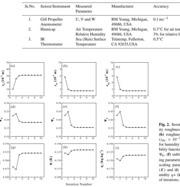
0 2 4 6 8 10 0 10 20 30 40 50 (a) z0 (1 0 -5 m) 0 2 4 6 8 10 0 2 4 6 8 10 (b) z0t (1 0 -5 m) 0 2 4 6 8 10 0 2 4 6 8 10 (c) z0q (1 0 -5 m) 0 2 4 6 8 10 0.10 0.15 0.20 0.25 0.30 (d) ψψψψm 0 2 4 6 8 10 0.30 0.35 0.40 0.45 0.50 (e) ψψψψh 0 2 4 6 8 10 0.30 0.35 0.40 0.45 0.50 (f) ψψψψq 0 2 4 6 8 10 0.450 0.475 0.500 0.525 0.550 (g) u* (m s -1 ) 0 2 4 6 8 10 -0.200 -0.175 -0.150 -0.125 -0.100 (h) Iteration Number θθθθ* (K ) 0 2 4 6 8 10 -0.200 -0.175 -0.150 -0.125 -0.100 (i) q* (k g .k g -1 )

Fig. 2. Iterative estimates of (a)

veloc-ity roughness length (z0, × 10−5 m),

(b) roughness length for temperature

(z0t, × 10−5m), (c) roughness length

for humidity (z_0q, × 10−5m), (d) sta-bility function 9m(e) stability function

9_h, (f) stability function 9q, (g)

scal-ing parameter for wind u∗ (ms−1), (h) scaling parameter for temperature θ ∗ (K)and (i) scaling parameter for hu-midity q∗ (kg.kg−1) with the number of iterations.

assumed applicable for the sea surface under moderate wind conditions (Lo, 1993). For the first iteration, the stability functions “9m”, “9t” and “9q” are assumed to be zero, the

wind speed at sea surface (US) is taken as zero (Lo, 1993)

and the relative humidity at the sea surface is assumed to be 98% (Kraus and Businger, 1994). The neutral stability trans-fer coefficients are uniquely related to the roughness lengths

z0x (z0 in case of wind profiles, z0t in case of temperature profiles and z0q in case of humidity profiles) as:

CxN = [k2/ln(z/z0).ln(z/z0x)]. (9)

Smith (1988) showed that the neutral stability transfer co-efficients for heat and moisture (CH Nand CEN) are

approxi-mately independent of wind speed with values of 1.15×10−3 at a reference height of 10-m. Therefore, solving the above equation for the roughness length, with the prescribed value

of (CH Nand CEN (= 1.15 × 10−3), we obtain the roughness

length for temperature and humidity (z0tand z0q) as: z0t=z0q =z/exp[k2/(1.15 × 10−3).ln(z/z0)]. (10)

With the estimates of friction velocity obtained from Eq. (1), we follow the empirical relation for roughness length suggested by Charnock (1955). The roughness length (z0) is represented as the sum of two terms, one due to Charnock (1955) (z0c =α.u ∗2/g)) and the other is the viscous term (z0s =β.υ/α.u∗) due to Smith (1988), (Fairall et al., 1996; Grachev and Fairall, 1997):

z0=(α.u ∗2/g) + (β.υ/α.u∗), (11)

where α is the Charnock “constant”, for which values be-tween 0.010 and 0.035 are cited in literature (Garratt, 1992, Table 4.1, pp. 99). In the present analysis, the value of

α is taken as 0.011 (after Smith, 1988). The term “υ” (= 14 × 10−6m2s−1) represents the dynamic viscosity of

D. B. Subrahamanyam and R. Ramachandran: Wind Speed dependence of Air-Sea Exchange parameters 1671 air. For wind speeds above about 6 ms−1_{, the second term in}

Eq. (11) is negligible. A value of β = 0.11 has been used from wind tunnel experiments following Smith et al. (1996). The roughness length (z0) estimate obtained from Eq. (11) is then substituted into Eq. (10) to obtain new estimates of roughness length for heat and moisture (z0t and z0q). The wind speed at the sea surface (Us), commonly known as drift

velocity, is taken as zero for the first iteration. Smith (1988) performed the above calculations for a range of wind speeds and sea-air (virtual) temperature differences by iterating u∗ and θ ∗ until the neutral flux coefficients matched their spec-ified values. Here, the value of the drift velocity (wind speed at sea surface, Us in Eq. 1) is taken as zero. However, it has

been verified experimentally and theoretically, that the sur-face drift velocity is approximately equal to u∗ (e.g. Hicks, 1972; Lo, 1993; Roll, 1965). Therefore, in the revised bulk algorithm (Subrahamanyam and Radhika, 2002), the itera-tion is carried out for obtaining the estimates of u∗, θ ∗ and

q∗in such a way that for all subsequent iterations the esti-mated value of u∗ from the preceding iteration is substituted in place of drift velocity (Us). The integrated stability

func-tions (9m, 9t and 9q) are estimated using equations

sug-gested in Smith (1988). Now, the estimated values of rough-ness lengths (z0, z0tand z0q) and the stability functions (9m, 9t and 9q) are substituted into Eqs. (1), (2) and (3) to

deter-mine new estimates of u∗, θ ∗ and q∗. Using these, the sta-bility functions (9m, 9t and 9q) and the roughness lengths

(z0, z0t and z0q) are determined again and the iteration is re-peated, untill the u∗, θ ∗, q∗ and z0calculated from the two consecutive iterations converge. Figure 2 shows the gradual convergence of the estimates of the roughness lengths (z0, z0tand z0q) shown in Figs. 2a, b and c, respectively), the sta-bility functions (9m, 9t and 9q) shown in Figs. 2d, e and

f, respectively), and the scaling parameters (u∗, θ ∗ and q∗ shown in Figs. 2g, h and i, respectively), through the itera-tions. The iterative method has two main advantages: (1) the surface drift velocity is taken as zero only for the first iter-ation, afterwards it is replaced by u∗, thereby giving better and more accurate values of other parameters in the ensuing iterations; (2) for initialing the calculations, the sea surface roughness length (z0) is taken as 10−4-m (Lo, 1993). How-ever, an estimate of z0 based on the iteration of the surface layer data collected during the INDOEX campaign covering a broad oceanic region will be a better representation of ac-tual z0against the initially assumed value of 10−4 m. Fig-ure 2 represents the converging values of the estimates after successive iterations. These final estimates of u∗, θ ∗ and

q∗are then used for the computation of the drag coefficient (CD) and sensible heat and water vapour exchange

coeffi-cients (CH and CE) as follows (Byun, 1990; DeCosmo et

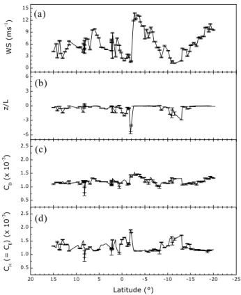
al., 1996): CD=u ∗2/(U10−Us)2 (12) CH =u ∗ .θ ∗ /(U10−Us).(θ10−Ts) (13) CE =u ∗ .q ∗ /(U10−Us).(q10−qs). (14) 20 15 10 5 0 -5 -10 -15 -20 -25 0.5 1.0 1.5 2.0 2.5 (d) CH (= CE ) ( x 1 0 -3) Latitude (°) 0.5 1.0 1.5 2.0 2.5 (c) CD (x 1 0 -3) -6 -3 0 3 6 (b) z/ L 0 3 6 9 12 15

Cruise leg-1 (January 20 - February 04, 1999)

(a)

WS

(m

s

-1)

Fig. 3. Latitudinal variation of air-sea interaction parameters along

cruise leg-1. (a) Wind Speed (W S, ms−1); (b) Stability Parameter (z/L); (c) Drag Coefficient (CD, × 10−3); (d) Sensible Heat and

Water Vapour exchange coefficients (CHand CE, × 10−3).

4 Results and discussion

The meteorological conditions prevailing over the region of tropical Indian Ocean and Central Arabian Sea along the cruise tracks during the entire campaign can be summarized as follows: during the forward track of the cruise, most of the days were cloudy. Along leg-1, heavy rains were observed in the latitude range 2◦S to 4◦S. During leg-3 and leg-4, i.e. the return track of the cruise, barring a few days, most of the days were clear, bright and sunny. During the INDOEX, IFP-99 (20 January– 12 March 1IFP-999), the Inter-Tropical Conver-gence Zone (ITCZ) was located in the Southern Hemisphere, around 5◦S and was migratory (Madan et al., 1999). Subra-hamanyam and Radhika (2002) have described the prevailing meteorological conditions in terms of surface observations along the cruise track in detail. Since the aim of this paper is to study the wind speed dependence of air-sea exchange parameters, we present the spatio-temporal variation of these parameters along the cruise track with the variation of wind speed. In the following sub-sections, we shall describe the spatio-temporal variation of boundary layer parameters along the cruise track (Figs. 3–6, respectively). In each of these figures, four panels (a–d) represent the spatio-temporal vari-ation of the following parameters: (a) Wind Speed (W S, ms−1); (b) Stability Parameter (z/L); (c) Drag Coefficient

1672 D. B. Subrahamanyam and R. Ramachandran: Wind Speed dependence of Air-Sea Exchange parameters 56 58 60 62 64 66 68 70 72 74 76 78 80 0.5 1.0 1.5 2.0 2.5 (d) CH (= CE ) ( x 10 -3) Longitude (°) 0.5 1.0 1.5 2.0 2.5 (c) CD (x 1 0 -3) -6 -3 0 3 6 (b) z/ L 0 3 6 9 12 15

Cruise leg-2 (February 04 - 11, 1999)

(a)

WS

(m

s

-1 )

Fig. 4. Longitudinal variation of air-sea interaction parameters along cruise leg-2. (a) Wind Speed (W S, ms−1); (b) Stability Pa-rameter (z/L); (c) Drag Coefficient (CD, × 10−3)); (d)

Sensi-ble Heat and Water Vapour exchange coefficients (CH and CE, ×

10−3).

(CD); (d) Sensible Heat and Water Vapour exchange

coeffi-cients (CH and CE), respectively. The error bars represent

the uncertainty in the measurements and the estimated pa-rameters due to uncertainty in the instrumentation errors. 4.1 Spatio-temporal variations in air-sea exchange

param-eters along the cruise track

4.1.1 Cruise leg-1 (meridional track-AB)

Figure 3 shows the latitudinal variation of air-sea interaction parameters along cruise leg-1, marked “AB” in Fig. 1a. This part of the cruise was traversed in a period of almost 15 days from 21 January–4 February 1999. During this leg, the ITCZ was located between the equator and 10◦_{S. Intense}

convec-tion and associated rainfall are also reported in this latitudinal belt (Subrahamanyam et al., 2002, 2003). Along the cruise leg-1, W S varied within a range 1 to 14 ms−1, with a peak value of about 14 ms−1between the equator and the 3◦S lat-itudinal belt (Fig. 3a). As the ship crossed 10◦S latitude, it experienced a gradual increase in W S magnitudes and be-came maximum at the tip of the leg at 20◦S, i.e. at point “B” (Fig. 1a). The weekly averaged wind field analysis provided by the National Centre for Medium Range Weather Fore-casting (NCMRWF, New Delhi, India) reported by Madan

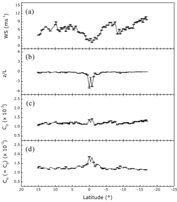
20 15 10 5 0 -5 -10 -15 -20 -25 0.5 1.0 1.5 2.0 2.5 (d) CH (= C E ) ( x 1 0 -3 ) Latitude (°) 0.5 1.0 1.5 2.0 2.5 (c) CD (x 1 0 -3) -6 -3 0 3 6 (b) z/ L 0 3 6 9 12 15

Cruise leg-3 (February 18 - March 01, 1999)

(a)

WS

(m

s

-1)

Fig. 5. Same as Fig. 3, but for cruise leg-3.

et al. (1999) also supports the surface observations shown in these figures (Subrahamanyam and Radhika, 2002). Fig-ure 3b shows the latitudinal variation in stability parame-ter values (z/L). The Monin-Obukhov stability parameparame-ter (z/L) is a measure of atmospheric stability. Negative values of z/L correspond to unstable conditions while positive val-ues represent stable conditions (Stull, 1988). Except for a few regions, the entire cruise leg-1 experienced near-neutral conditions, with z/L ≈ 0. Panels “c” and “d” of Fig. 3 shows the variation in air-sea exchange coefficients, CDand

(CH =CE), respectively. A small change in the magnitudes

of these coefficients can lead to a large variation in the flux magnitudes. Along cruise leg-1, on average, CDvalues were

about 1.20 while CH values were about 1.26 (Figs. 3c and d).

It has to be noted that along ITCZ regions near the equatorial belt, the air-sea exchange coefficients also show considerable gradients, which, in turn, affect the magnitudes of air-sea in-terface fluxes over these regions.

4.1.2 Cruise leg-2 (zonal track-BC)

Longitudinal variation of observed and estimated parameters along cruise leg-2 is shown in Fig. 4. Cruise leg-2 (marked “BC” in Fig. 1a) took place between 4–11 February 1999. The fact that this part of the cruise took place within a period of a week and also that it had a zonal movement, one does not observe a drastic spatial variation in the observed parameters or in the estimates. As can be seen from the figure,

mag-D. B. Subrahamanyam and R. Ramachandran: Wind Speed dependence of Air-Sea Exchange parameters 1673 56 58 60 62 64 66 68 70 72 74 76 78 80 0.5 1.0 1.5 2.0 2.5 (d) CH (= CE ) ( x 1 0 -3) Longitude (°) 0.5 1.0 1.5 2.0 2.5 (c) CD (x 1 0 -3) -6 -3 0 3 6 (b) z/ L 0 3 6 9 12 15

Cruise leg-4 (March 01 - 06, 1999) (a)

WS (m

s

-1)

Fig. 6. Same as Fig. 4, but for cruise leg-4.

nitudes of wind speed were larger along leg-2, and broadly it varied within a range of 4.6 to 13 ms−1, with an average value of about 9.5 ms−1 (Fig. 4a). It has to be noted that the wind field analysis provided by NCMRWF, New Delhi (Madan et al., 1999) for the same period also shows strong easterly winds prevailing over this zonal belt. The stability parameter (z/L) and the air-sea exchange coefficients (CD

and CH) do not show any large variations along leg-2; z/L

values remained near zero, showing near-neutral stability of the atmosphere (Fig. 4b). Average drag coefficient values were about 1.31 (Fig. 4d) while CH values were about 1.18

(Fig. 4d).

4.1.3 Cruise leg-3 (meridional track-CD)

Figure 5 shows the latitudinal variation of air-sea interac-tion parameters for leg-3 covered during the return track of the cruise. This leg (marked “CD” in Fig. 1a) was tra-versed during 18 February–1 March 1999. It is to be noted that the prevailing conditions were different from that dur-ing the first meridional track-AB, which took place about 2–3 weeks earlier. Also, the second meridional track was along 63◦E against 77◦E longitude for the first meridional track. Most of the days during leg-3 were cloud free, bright and sunny. However, the ITCZ had weakened and its posi-tion was between the equator and the 10◦S latitudinal belt. Moderate to high wind speeds were observed along leg-3 of the cruise track. The southern part of leg-3 experienced large winds while the equatorial belt experienced low winds

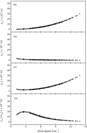
0 3 6 9 12 15 0 10 20 30 40 50 (d) z0t (= z0q ) ( x 1 0 -5 m) Wind Speed (ms-1 ) 0 10 20 30 40 50 (c) z0 ( x 10 -5 m) 0 10 20 30 40 50 (b) z0s ( x 1 0 -5 m) 0 10 20 30 40 50 _(a) z0c ( x 1 0 -5 m)

Fig. 7. Wind speed dependence of roughness length: (a)

Veloc-ity roughness length - z0c(×10−5m) (after Charnock, 1955); (b)

Velocity roughness length - z0s(×10−5m) (after Smith, 1988); (c)

Velocity roughness length z0 (sum of z0c and z0s), (×10−5m);

(d) Roughness length for temperature (and humidity) z0t (= z0q),

(×10−5m).

(Fig. 5a). Except for regions near the equator, the stability parameter and air-sea exchange coefficients remained con-stant (Figs. 5b, c and d). Drag coefficient values were about 1.21, while CH remained more or less constant with a value

of about 1.27 (Figs. 5c and d). 4.1.4 Cruise leg-4 (zonal track-DE)

Figure 6 shows the longitudinal variation of the air-sea in-teraction parameters for leg-4, covered between 1–6 March 1999. As for the longitudinal variations observed along leg-2, this leg also does not show large spatial gradients in air-sea exchange parameters. Along leg-4 wind speed magnitudes were low in the range 1.5 to 7.2 ms−1(Fig. 6a). The eastern sector of leg-4 shows unstable atmospheric conditions with negative values of z/L (Fig. 6b). Figures 6c and d show the longitudinal variation of CDand CH, respectively. From the

figure, it can be seen that there is no large variation in the parameters as was seen in the meridional tracks.

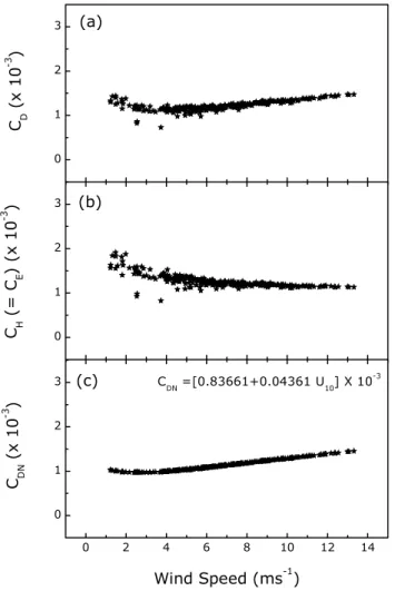
1674 D. B. Subrahamanyam and R. Ramachandran: Wind Speed dependence of Air-Sea Exchange parameters 0 2 4 6 8 10 12 14 0 1 2 3 _(c) C_DN =[0.83661+0.04361 U₁₀] X 10-3 C DN (x 1 0 -3 ) Wind Speed (ms-1) 0 1 2 3 (b) C H (= C E ) ( x 1 0 -3 ) 0 1 2 3 (a) C D (x 1 0 -3 )

Fig. 8. Wind speed dependence of air-sea exchange coefficients: (a)

CH(= CE); (b) CDand (c) CDN.

4.2 Variation of surface roughness length (z0, z0t and z0q) Now with the available estimates of air-sea exchange param-eters, we attempt to study the wind speed dependence of surface roughness length and air-sea exchange coefficients, imperative in the estimation of air-sea interface fluxes. The roughness length (z0x) can be physically interpreted as the virtual origins of the profiles of the concerned parameter “x” (in this case, “x” can be winds, temperature or humidity). It can be determined by plotting ln(z) vs. the measured winds at that height, and extrapolating the best-fit straight line down to the level where the winds are zero, with its intercept on the ordinate axis being ln(z0). One should note that this is only a mathematical or graphical procedure for estimating the roughness length (z0). In practice, measurements of any meteorological parameter over the oceanic surface at various heights are quite difficult. Therefore, in the present study, the roughness length is estimated using an iterative scheme described in Sect. 3.

We now attempt to study the variation of surface rough-ness length in relation to the surface wind speeds. Fig-ure 7 shows the wind speed dependence of velocity rough-ness length z0. As per the definition of velocity roughness

length (see Eq. (11), Sect. 3), z0c is given as the sum of two terms, z0c and z0s. The variation of the two indepen-dent terms, z0cand z0s are shown separately in the top two panels (Figs. 7a and b), followed by the variation of z0and z0t (= z0q) in the two bottom panels (Figs. 7c and d). From Fig. 7a, it is clear that there is a significant increase in the roughness z0c(defined by Charnock, 1955) with increasing wind speed. In contrast to the variation of the first term z0c, we see a decreasing trend for the variation of second term

z0s (the viscous term defined by Smith, 1988) with increas-ing wind speed (Fig. 7b). It can be seen from Fig. 7b that for winds above 6 ms−1, as expected, the viscous term (z0s) has negligible influence, and the value drops to zero in large winds and it dominates in the lower wind speed regime. The variation of velocity roughness length, which is defined as the sum of z0cand z0s, with wind speed, is shown in Fig. 7c with the variation of wind speed. The wind speed depen-dence of z0reflects the behaviour of both the terms collec-tively. From Fig. 7c, we can see that the magnitude of ve-locity roughness length (z0) decreases from 9 × 10−5m to 3 ×10−5m, when the magnitude of the winds changed from 1 ms−1to 3 ms−1. Once it exceeds a value of 3 ms−1, there is a sharp increase in the magnitude of z0, and it reaches up to 30 × 10−5m at about 14 ms−1. Figure 7d shows the vari-ation of roughness lengths for temperature and humidity (z0t and z0q) with increasing wind speed. When the winds are greater than 3 ms−1, there is clear evidence that the surface roughness for temperature and humidity decreases with in-creasing wind speed. However, in the wind speed regime of 0 to 3 ms−1, there is a sharp increase in the magnitude of z0t (= z0q) with increasing wind speeds. This behaviour of z0t and z0q at lower wind speeds can again be explained due to the viscous term, shown in Eq. (11), which determines the magnitude of z0. When we compare the variation of z0and z0t (= z0q) with wind speed, we notice that for low winds (when winds are less than 7 ms−1), the magnitudes of z0t (= z0q) are large compared to z0; however, at larger wind speeds (>7 ms−1), the z0values are considerably larger than that of the z0t(=z0q) values.

Malhi (1996) gives a detailed analysis of the behaviour of the roughness length for temperature (z0t) over hetero-geneous surfaces over land. His analysis demonstrated that certain transfer processes within the interfacial sub-layer, no-tably molecular diffusion and free convection, might induce a dependency of z0ton wind speed. Furthermore, in this study the roughness length for temperature (z0t) shows a decreas-ing trend with increasdecreas-ing wind speed. Except for the lower wind speed regime (0 to 3 ms−1_{), our analysis also shows a} decreasing trend for z0t and z0q with increasing wind speed. Turbulence alone cannot transfer heat and moisture over the air-sea interface; therefore, we have to consider molecular effects, in addition to turbulent transfer, for studying the be-haviour of z0t and z0q. Molecular conduction of heat and molecular diffusion of tracers cause transport between the surface and the lowest few millimeters of air. With increasing wind speed, the formation of sea waves lead to dominance of turbulence over molecular diffusion at the lowest few

cen-D. B. Subrahamanyam and R. Ramachandran: Wind Speed dependence of Air-Sea Exchange parameters 1675 timeters of air, which would lead to a further decrease in the

magnitude of z0t and z0q.

4.3 Variation of air-sea exchange coefficients

Figure 8 shows the wind speed dependence of bulk trans-fer coefficients for momentum, heat and moisture computed using Eqs. (12) to (14). In the figure, the top panel (8a) shows the wind speed dependence of drag coefficients and Fig. 8b that of the sensible heat and water vapor exchange coefficients. From Fig. 8a, we notice that the drag coef-ficient increases with increasing wind speed. Over a wind speed regime of 1–14 ms−1_{(observed during INDOEX,} IFP-99 campaign), the variation of drag coefficient lies within a range 0.7–1.5 (× 10−3_{); however, in the lower wind speed} regime (i.e. 1–4 ms−1), there is a slight decrease in the magnitude of drag coefficient. Smith (1988) also reported a similar variation of drag coefficient at a lower wind speed regime. He observed that the value of the exchange coeffi-cient depends strongly on the stability stratification at low wind speeds, but such an influence was not seen with in-creasing wind speed. Recently, Wu (1994) suggested that the closely packed capillary waves associated with surface ten-sion partly explain the large drag coefficients at weak winds. Geernaert et al. (1988), Bradley et al. (1991) and Greenhut and Khalsa (1995) have also reported a similar increase in drag coefficient values at low wind speeds. In contrast to the variation of drag coefficient (CD), in Fig. 8b, we observe that

the magnitude of CH (= CE) decreases with increasing wind

speed. At larger wind speeds, it becomes almost constant and there is very little scatter at these wind speeds, whereas large scatter can be seen in the lower wind speed regime. Bradley et al. (1991) pointed out that the large scatter in the measured values of CH can arise because of the very low heat fluxes,

about the order of what can be obtained at the limit of reso-lution of the turbulence measurements. However, it is worth mentioning that the estimates of the air-sea exchange coef-ficients are strongly dependent on the bulk scheme adopted and its dependence on stability. Table 2 compares the es-timates of the air-sea exchange coefficients of sensible heat (CH) and water vapour (CE) obtained in the present study

with those obtained by other investigators.

Using the bulk transfer coefficients already obtained, we now attempt to study the variation of these coefficients for neutral stratification. The expression for neutral stability transfer coefficient (shown in Eq. 4, Sect. 3) is hypothetical, since neutral stability implies zero heat flux at the surface and a nonexistent potential temperature gradient (Bradley et al., 1991). In the revised bulk scheme adopted for the present analysis, the neutral stability transfer coefficients for heat and moisture (CH N = CEN) are taken as constants with a

prescribed value of 1.15 × 10−3 (Smith, 1988). Now we study the variation of neutral drag coefficient (CDN) with

respect to the wind speed over the Indian Ocean. We un-derstand from Fig. 8c that for the larger wind speed regime (>4 ms−1), there is a significant increase in the magnitudes of CDN (from 0.85 to 1.5 × 10−3, which implies that with

increasing wind speed, the sea surface roughness also in-creases). The increase in the magnitude of CDN at low wind

speeds can again be attributed to the viscous term defined in Eq. (11) (Sect. 3). Based on the scatter plot of CDN vs. wind

speed, we have derived an empirical relation between our es-timates of CDNwith the observed values of wind speeds. The

equation representing the best fit is also shown in the figure, to arrive at the following empirical relationship for CDN: CDN = [(0.8366 ± 0.0423)

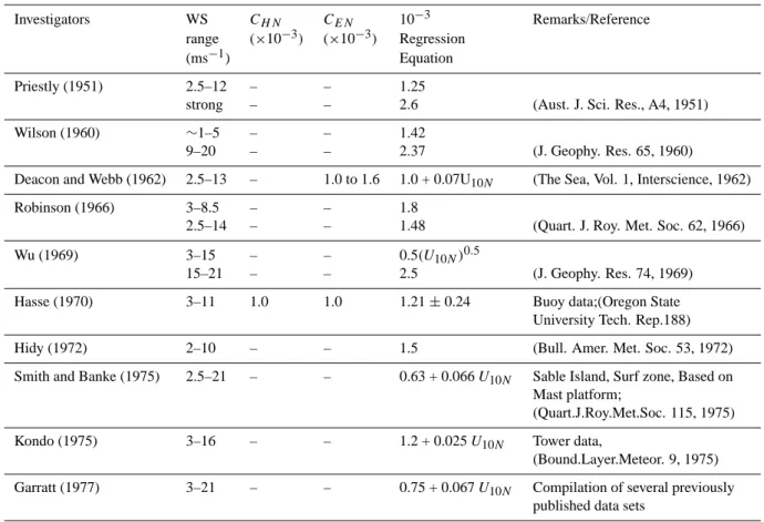
+(0.0436 ± 0.0005) × U10] ×10−3. (15) DeCosmo (1991) gives a comparison of the various re-gression estimates of drag coefficients at 10-m height. A few CDN regression equations with the respective range of

wind speeds reported by DeCosmo (1991), Garratt (1977) and the present study are detailed in Table 2. These equa-tions, derived empirically, spread over a wide range of wind speeds. Equation (15) gives the wind speed dependence of drag coefficient for neutral stratification over a wind speed range, 1–14 ms−1. Stull (1988) gives the average magni-tudes of drag coefficients over different continents (see Ta-ble 7-2, pp. 264). Several studies suggested that the vari-ance in the drag coefficient estimates may be explained pri-marily by an additional dependence of CDon sea state, but

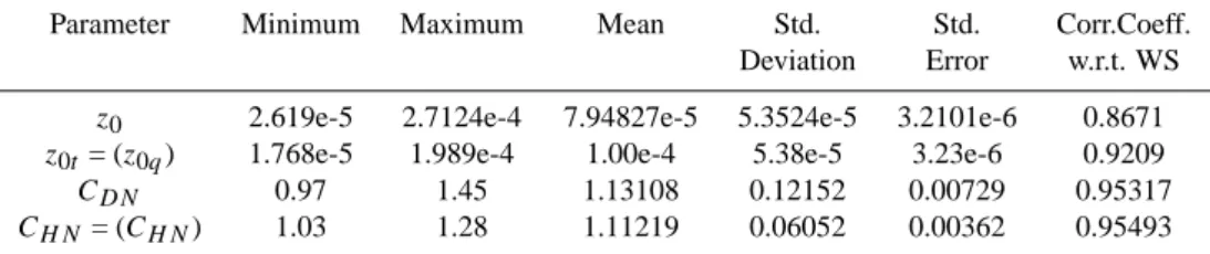
the mathematical formulation which best describes this rela-tionship for non-equilibrium conditions is not readily agreed upon by many investigators. To summarize the behaviour of air-sea exchange parameters over the tropical Indian Ocean and Central Arabian Sea during the INDOEX, IFP-99 cam-paign and their wind speed dependence, the statistical esti-mates and the errors in the estiesti-mates are given in Table 3.

5 Summary

In the present study, the wind speed dependence of air-sea exchange coefficients over the Indian Ocean during the IN-DOEX, IFP-99 campaign is reported. The magnitude of the exchange coefficient depends on many factors, includ-ing the wind speed, fetch and wave age, stability, the scheme adopted for the estimation of these coefficients, etc. In this study, however, we have attempted to show only the wind speed dependence of the air-sea exchange parameters. The key features revealed from the study can be summarized as follows:

– The drag coefficient estimates for neutral stratification

increases at low wind speeds, typically in the range 1– 4 ms−1_.

– For larger winds (>4 ms−1), there is a significant in-crease in the magnitude of the neutral drag coefficient, and the coefficients show an increasing trend with in-creasing wind speed.

– In contrast to the variation of drag coefficient, the

1676 D. B. Subrahamanyam and R. Ramachandran: Wind Speed dependence of Air-Sea Exchange parameters

Table 2. Review on comparison of estimates in air-sea exchange coefficients (CH and CE) and regression of drag coefficient for neutral

stratification (CDN) based on wind speed at 10-m

Investigators WS CH N CEN 10−3 Remarks/Reference

range (×10−3) (×10−3) Regression (ms−1) Equation Priestly (1951) 2.5–12 – – 1.25

strong – – 2.6 (Aust. J. Sci. Res., A4, 1951) Wilson (1960) ∼1–5 – – 1.42

9–20 – – 2.37 (J. Geophy. Res. 65, 1960)

Deacon and Webb (1962) 2.5–13 – 1.0 to 1.6 1.0 + 0.07U10N (The Sea, Vol. 1, Interscience, 1962)

Robinson (1966) 3–8.5 – – 1.8

2.5–14 – – 1.48 (Quart. J. Roy. Met. Soc. 62, 1966) Wu (1969) 3–15 – – 0.5(U_10N)0.5

15–21 – – 2.5 (J. Geophy. Res. 74, 1969) Hasse (1970) 3–11 1.0 1.0 1.21 ± 0.24 Buoy data;(Oregon State

University Tech. Rep.188) Hidy (1972) 2–10 – – 1.5 (Bull. Amer. Met. Soc. 53, 1972) Smith and Banke (1975) 2.5–21 – – 0.63 + 0.066 U10N Sable Island, Surf zone, Based on

Mast platform;

(Quart.J.Roy.Met.Soc. 115, 1975) Kondo (1975) 3–16 – – 1.2 + 0.025 U10N Tower data,

(Bound.Layer.Meteor. 9, 1975) Garratt (1977) 3–21 – – 0.75 + 0.067 U10N Compilation of several previously

published data sets

do not show any significant variation with increasing wind speed in the wind speed range 1–14 ms−1_{. An} av-erage value of the exchange coefficients are:

– CH N (= CEN) = 1.11 ± 0.06.

– Estimates of the drag coefficient for neutral

stratifica-tion over the Indian Ocean using the present scheme, provide the following regression equation for CDN with

wind speed:

– CDN = [0.8366 + 0.0436 × U10] ×10−3.

– Except for low winds (<3 ms−1), the velocity rough-ness length (z0) increases with increasing wind speed. In contrast, the roughness length for temperature and humidity (z0tand z0q) show a decreasing trend with in-creasing wind speed (>3 ms−1).

6 Concluding remarks

The INDOEX, IFP-99 campaign provided an opportunity to study the structure and characteristics of MABL over the In-dian Ocean. In the present article, some of the features of

air-sea interaction over the Indian Ocean are addressed. Air-sea exchange parameters of water vapor, heat and momen-tum are important inputs for mesoscale and GCM model-ing. These are particularly lacking over the tropical oceans. Various schemes were published from time to time for the computation of bulk transfer coefficients. There are several studies that report MABL characteristics over oceans; such studies over the tropical Indian Ocean region, however, are few. In the present study, an attempt is being made to show the behaviour of the surface roughness length and air-sea ex-change coefficients from data collected over a wide region of the tropical Indian Ocean during INDOEX, IFP-99 cam-paign. Webster and Lukas (1992) emphasized that “the vari-ation of fluxes between the ocean and the atmosphere is very sensitive to the choice of parameterization, especially in low wind regimes.” Miller et al. (1992), who found dramatic im-provements in simulated tropical phenomena by strengthen-ing the air-sea couplstrengthen-ing in the light wind regime, verifies this fact. In low wind speed regimes it is necessary to account for buoyancy effects on the turbulent transport, an aspect that is dealt with in the standard stability dependent bulk scheme adopted by Smith (1988), which shows a good performance in the tropics (Bradley et al., 1991). Estimates of bulk trans-fer coefficients and roughness lengths for velocity,

tempera-D. B. Subrahamanyam and R. Ramachandran: Wind Speed dependence of Air-Sea Exchange parameters 1677

Table 2. continued....

Investigators WS CH N CEN 10−3 Remarks/Reference

range (×10−3) (×10−3) Regression

(ms−1) Equation

Pond et al. (1971) 4–8 1.0 1.23±0.17 1.5 × 10−3 Large buoy data; Comparison of 1.25±0.25 eddy correlation and inertial

dissi-pation method. (J.Atmos.Sci.28, 1971) Large and Pond 10–25 – – 0.49 + 0.065U10N Compilation of ocean measurements

(1981, 1982)

Donelan (1982) 4–16 – – 0.35 + 0.142 U10N Lake Ontario, 10 m

Geernaert et al. (1986) 5–22 – – 0.40 + 0.117 U10N North Sea, 15 m

Geernaert et al. (1987) 5–25 – – 0.577 + 0.085 U10N North Sea, 30 m

Smith (1988) 6–22 1.0 1.2 0.81 + 0.049 U10N North Atlantic, Deep water

Bradley et al. (1991) 4–6 1.03 0.89 1.16 Micrometeorological measurements carried onboard R/V Franklin over the western equatorial pacific ocean Large et al. (1994) 1–25 32.7 (CD)1/2 (2.7/U10N+0.142

unstable 34.6(C_D)1/2

18.0(CD)1/2 + 0.0764 U10N (Reviews of Geophysics.)

stable 32/4, 1994

DeCosmo et al. (1996) 5–23 1.14 1.12 0.27 + 0.116 U10N HEXOS results

Enriquez and 2–17 1.05± 0.39 – 0.509 + 0.065 U_10N Aircraft measurements during Friehe (1997) SMILE, (J.Geophy.Res. 102, 1997) Enriquez and 2–17 – – 0.6492 + 0.0571 U_10N Aircraft measurements during Friehe (1997) CODE, (J.Geophy.Res. 102, 1997) Rutgersson et al. 2–15 1.0 ± 0.3 1.2 ± 0.2 – Baltic Sea measurements,

(2001) (Bound.Layer.Meteorol. 99, 2001)

Subrahamanyam and 1–14 1.11 ± 0.06 1.11 ± 0.06 0.8366 + 0.0436 U_10N Western Tropical Indian Ocean Radhika, (Present Study) during INDOEX, IFP-99

Table 3. Statistical estimates of parameters and their wind speed dependence during INDOEX, IFP-99

Parameter Minimum Maximum Mean Std. Std. Corr.Coeff. Deviation Error w.r.t. WS z0 2.619e-5 2.7124e-4 7.94827e-5 5.3524e-5 3.2101e-6 0.8671

z0t= (z0q) 1.768e-5 1.989e-4 1.00e-4 5.38e-5 3.23e-6 0.9209

CDN 0.97 1.45 1.13108 0.12152 0.00729 0.95317

CH N= (CH N) 1.03 1.28 1.11219 0.06052 0.00362 0.95493

ture and humidity over the Indian Ocean are obtained using a method based on the bulk algorithm suggested by Smith (1988). A modification is suggested in this work to the bulk algorithm suggested by Smith (1988) by way of iteratively computing u∗, z0, z0t and z0q. It has effectively improved the accuracy of the estimates of the exchange coefficients, in turn, providing a fairly reliable estimate of the fluxes.

Our estimates of the drag coefficients, particularly over the meridional tracks, could have an inherent error since it is cross-equatorial, where one can expect large gradients. The general assumption of a homogeneous boundary layer, in this case, may not be valid. Relatively large variability in the meridional track estimates against zonal track estimates, par-ticularly in consonance with large SST and wind speed

gra-1678 D. B. Subrahamanyam and R. Ramachandran: Wind Speed dependence of Air-Sea Exchange parameters dients, evident in this study, point to this fact. Hence, to that

extent there is a limitation in the accuracy of the estimates of the parameters along the meridional track reported in this study.

Although there is a general agreement among investiga-tors that the wind drag coefficient increases with increasing wind speed over the ocean, there is also a strong view against the empirically determined coefficients of the simple linear formula, which quantifies this relationship. This can be at-tributed to the inefficient calibration and other errors due to sensor deployment caused by flow distortion, violation of the assumptions of steady state and of isotropic turbulence and the underlying physics of the scheme adopted for estimating the bulk transfer coefficients. Concerted effort, by way of both research and field experiments, are necessary to further strengthen our understanding of the boundary layer parame-terization and the bulk schemes over the tropical oceans.

Acknowledgements. We acknowledge with thanks the help

ren-dered by Dr. K Sen Gupta, Former-Head, Boundary Layer Physics (BLP) Branch, Space Physics Laboratory, Vikram Sarabhai Space Centre, Thiruvananthapuram for initiating the BLP component of the INDOEX programme. We are grateful to Dr. A.P. Mitra, Chair-man, National Steering Committee, Shri G. Viswanathan, Program Director, INDOEX-India Program, Dr. N. Bahulayan, Chief Scien-tist onboard ORV Sagar Kanya and all the members of the Indian component of INDOEX program for their strenuous efforts for mak-ing the Indian component of the campaign a great success. Thanks are also due to the anonymous reviewers for their critical appraisal of the manuscript, which in turn, improved the contents of the pa-per to a great extent. One of the authors, Subrahamanyam, who was a participant in the INDOEX, IFP-99 campaign, is thankful to the Indian Space Research Organization (ISRO) for providing the Re-search Fellowship for carrying out this reRe-search.

Topical Editor N. Pinard’e thanks two referees for their help in evaluating this paper.

References

Blanc, T. V.: Accuracy of Bulk-Method-Determined Flux, Stability, and Sea Surface Roughness, J. Geophys. Res., 92, 3867–3876, 1987.

Blanc, T. V.: Variation of bulk-derived surface flux, stability and roughness results due to the use of different transfer coefficient schemes, J. Phys. Ocean., 15, 650–659, 1985.

Bradley, E. F., Coppin, P. A., and Godfrey, J. S.: Measurements of sensible and latent heat flux in the western equatorial Pacific Ocean, J. Geophys. Res., 96, 3 375–3 389, 1991.

Businger, J. A., Wyngaard, J. C., Izumi, Y., and Badgley, E. F.: Flux profile relationships in the atmospheric surface layer, J. Atmos. Sci., 28, 181–189, 1971.

Byun, D. W.: On the analytical solutions of flux-profile relation-ships for the atmospheric surface layer, J. Applied Meteo., 29, 652–657, 1990.

Charnock, H.: Wind stress on the water surface, Q. J. R. Meteo. Soc., 81, 639–640, 1955.

Deacon, E. L. and Webb, E. K.: Interchange of properties between sea and air, The Sea, Vol. 1, Interscience, 43–87, 1962.

Dyer, A. J.: A review of flux-profile relationships, Boundary Layer Meteorology, 7, 363–372, 1974.

DeCosmo, J.: Air-Sea Exchange Of Momentum, Heat And Water Vapor Over Whitecap Sea States, Ph.D. Dissertation, University of Washington, Seattle, WA 98165, 212 pp., 1991.

DeCosmo, J., Kastaros, K. V., Smith, S. D., Anderson, R. J., Oost, W. J., Bumke, K., and Chadwick, H.: Air-Sea Exchange of water vapor and sensible heat: The Humidity Exchange Over the Sea (HEXOS) results, J. Geophys. Res., 101, 12 001–12 016, 1996. Donelan, M.: The dependence of the aerodynamic drag coefficient

on wave parameters, First International Conference on Meteo-rology and Air-Sea Interaction of the Coastal Zone, American Meteorological Society, Boston, MA, pp. 381–287, 1982. Enriquez, A.G. and Friehe: C.A., Bulk parameterization of

momen-tum, heat, and moisture fluxes over a coastal upwelling area, J. Geophys. Res., 102, 5781–5798, 1997.

Fairall, C. W., Bradley, E. F., Rogers, D. P., Edson, J. B., and Young, G. S.: Bulk parameterization of air-sea fluxes for Tropi-cal Oceans and Global Atmosphere Coupled Ocean-Atmosphere Response Experiment, J. Geophys. Res., 101, 3 747–3 764, 1996. Friehe, C. A. and Schmidt, K. F., Parameterization of air-sea inter-face fluxes of sensible heat and moisture by the bulk aerodynamic formulas, J. Phys. Ocean., 6, 801–809, 1976.

Garratt, J. R.: Review of drag coefficients over oceans and conti-nents, Monthly Weather Review, 105, 914–929, 1977.

Garratt, J. R.: The Atmospheric Boundary Layer, Cambridge Uni-versity Press, Cambridge, 316 pp., 1992.

Geernaert, G. L., Davidson, K. L., Larsen, S. E., and Mikkelsen, T.: Wind stress measurements during the Tower Ocean Wave and Radar Dependence Experiment, J. Geophys. Res., 93, 13 913– 13 923, 1988.

Geernaert, G. L., Larsen, S. E., and Hansen, F.: Measurements of the wind stress, heat flux, and turbulence intensity during storm conditions over the North Sea, J. Geophys. Res., 92, 13 127– 13 139, 1987.

Geernaert, G. L., Katsaros, K. B., and Richter, K.: Variation of the drag coefficient and its dependence on sea state, J. Geophys. Res., 91, 7 667–7 679, 1986.

Grachev, A. A. and Fairall, C. W.: Dependence of the Monin-Obukhov Stability Parameter on the Bulk Richardson Number over the Ocean, J. Applied Meteo., 36, 406–414, 1997.

Greenhut, G. and Khalsa, S. J. S.: Bulk transfer coefficients and dissipation derived fluxes in low wind speed conditions over the western equatorial Pacific Ocean, J. Geophys. Res., 100, 857– 863, 1995.

Hasse, L.: On the determination of vertical transports of momentum and heat in the atmospheric boundary layer at sea, Tech. Rep. 188, Dept. of Oceanography, Oregon State University, 1970. Hicks, B. B.: Propeller anemometers as sensors of atmospheric

tur-bulence, Boundary Layer Meteorology, 3, 214–228, 1972. Hidy, G. M.: A view of recent air-sea interaction research, Bulletin

of American Meteorological Society, 53, 1083–1102, 1972. Kondo, J.: Air-sea bulk transfer coefficients in diabatic conditions,

Boundary Layer Meteorology, 9, 91–112, 1975.

Kraus, E. B. and Businger, J. A.: Atmosphere-Ocean Interactions, Second Edition, Oxford University Press, New York, 352 pp., 1994.

Large, W. G., McWilliams, J. C., and Doney, S. C., Ocean vertical mixing: A review and a model with a nonlocal boundary layer parameterization, Rev. Geophys., 32, 363–403, 1994.

Large, W. G. and Pond, S.: Open ocean momentum flux measure-ments in moderate to strong winds, J. Phys. Ocean., 11, 324–336, 1981.

measure-D. B. Subrahamanyam and R. Ramachandran: Wind Speed dependence of Air-Sea Exchange parameters 1679

ments over the ocean, J. Phys. Ocean., 12, 464–482, 1982. Lo, A. K-F.: The Direct Calculation of Fluxes and Profiles in the

Marine Surface Layer Using Measurements from a Single At-mospheric Level, J. Applied Meteo., 32, 1 893–1 900, 1993. Madan, O. P., Mohanty, U. C., Paliwal, R. K., et al.: Meteorological

Analysis during INDOEX, Intensive Field Phase – 1999, Volume – II: Wind Analysis and Trajectories, Centre for Atmospheric Sciences, IIT Delhi, Hauz Khas, New Delhi, 110016, 1999. Malhi, Y.: The behaviour of the roughness length for temperature

over heterogeneous surfaces, Q. J. R. Meteo. Soc., 122: 1095– 1125, 1996.

Miller, M. J., Beljaars, A. C. M., and Palmer, T. N.: The sensitiv-ity of the ECMWF model to the parameterization of evaporation from the tropical oceans, J. Climate, 5, 418–434, 1992. Paulson, C.A.: The mathematical representation of wind speed and

temperature profiles in the unstable atmospheric surface layer, J. Applied Meteo., 9, 857–861, 1970.

Pond, S., Phelps, G. T., Paquin, J. E., McBean, G., and Stewart, R. W.: Measurement of the turbulent fluxes of momentum, moisture and sensible heat over the oceans, J. Atmos. Sci., 28, 901–917, 1971.

Priestley, C. H. B.: A survey of the stress between the ocean and atmosphere, Australian J. Sci. Res., A4, 315–328, 1951. Ramanathan, V., Crutzen, P. J., Althausen, D., Anderson, J.,

An-dreae, M. O., Clarke, A. D., Collins, W. D., Coakley, J. A., Heymsfield, A. J., Holben, B., Jayaraman, A., Kiehl, J. T., Kr-ishnamurti, T. N., Lelieveld, J., Mitra, A. P., Novakov, T., Orgon, J. A., Podgorny, I. A., Prospero, J. M., Priestly, K., Quinn, P. K., Rajeev, K., Rasch, P., Rupert, S., Sadourney, R., Satheesh, S. K., Sheridan, P., Shaw, G. E., and Valero, F. P. J: The Indian Ocean experiment: wide spread haze from south and Southeast Asia and its climate forcing, J. Geophys. Res., 106, 28 371–28 398, 2001. Ramanathan, V., Coakley, J. A., Clarke, A., et al.: Indian Ocean Experiment (INDOEX); A Multi-agency proposal for Field Ex-periment in the Indian Ocean (C4 Publication No. 162, Scripps Institution of Oceanography, La Jolla, CA, 1996); also at (http://www.indoex.ucsd.edu), 1996.

Robinson, G. D.: Another look at some problems of the air-sea in-terface, Q. J. R. Meteo. Soc., 92, 451–465, 1966.

Roll, H. U.: Physics of the Marine Atmosphere, Academic Press, 426 pp., 1965.

Rutgersson, A., Smedman, A.-S., and Omstedt, A.: Measured and simulated latent and sensible heat fluxes at two marine sties in the Baltic sea, Boundary Layer Meteorology, 99, 53–84, 2001. Said, F. and Druilhet: A., Experimental Study of the Atmospheric

Marine Boundary Layer from in-situ aircraft measurements (TOSCANE-T CAMPAIGN): Variability of boundary conditions and Eddy flux parameterization, Boundary Layer Meteorology, 47, 277–293. 1991.

Smith, S. D.: Water vapor flux at the sea surface, Boundary Layer Meteorology, 47, 277–293, 1989.

Smith, S. D.: Wind stress and heat flux over the ocean in gale force winds, J. Phys. Ocean., 10, 709–726, 1980.

Smith, S. D., Fairall, C. W., Geernaert, G. L., and Hasse, L.: Air-Sea Fluxes: 25 Years of Progress, Boundary Layer Meteorology, 78, 247–290, 1996.

Smith, S. D.: Coefficients for Sea Surface Wind Stress, heat Flux, and Wind Profiles as a Function of Wind Speed and Temperature, J. Geophys. Res., 93, 15 467–15 472. 1988.

Smith, S. D. and Banke, E. G.: Variation of the sea surface drag coefficient with wind speed, Q. J. R. Meteo. Soc., 101, 665–673, 1975.

Stull, R. B.: An Introduction to Boundary Layer Meteorology, Kluwer Academic Publishers, P.O. Box 17, 3300 AA Dordrecht, The Netherlands, 666 pp., 1988.

Subrahamanyam, D. B. and Radhika, R.: Air-Sea Interface Fluxes over the Indian Ocean during INDOEX, IFP-99, J. Atmos.-Solar Terr. Phys., 64/3, 291–305, 2002.

Subrahamanyam, D. B., Radhika, R., Sen Gupta, K., Mandal, T. K.: Variability of Mixed Layer Heights over the Indian Ocean and Central Arabian Sea during INDOEX, IFP-99, Boundary Layer Meteorology, 107, 683–695, 2003.

Subrahamanyam, D. B., Radhika, R., Sen Gupta, K., Krishnan, P., Kunhikrishnan, P. K., and Ravindran, S.: Marine Atmospheric Boundary Layer (MABL) Studies over the Indian Ocean during INDOEX, IFP-99, SPL Scientific Report, Also available at: http: //www.geocities.com/subbu dbs/INDOEX/report ifp.pdf, 2002. Subrahamanyam, D. B., Sen Gupta, K., Ravindran, S., and

Krish-nan, P.: Study of sea breeze and land breeze along the west coast of Indian sub-continent over the latitude range 15◦N to 8◦N dur-ing INDOEX, IFP-99 (SK-141) cruise, Current Science (Supple-ment), 80, 85–88, 2001a.

Subrahamanyam, D. B., Sen Gupta, K., Ravindran, S., Kunhikr-ishnan, P. K., Radhika, R., Ramana, M. V., and KrKunhikr-ishnan, P.: Variation of Marine Atmospheric Boundary Layer Parameters in the Latitude Range 15◦N to 20◦S and Longitude Range 63◦E to 77◦E During INDOEX, IFP-99, Proceedings of the Sympo-sium TROPMET 2000 on Ocean and Atmosphere, IMS (Cochin Chapter), CUSAT, Cochin – 682 016, Kerala, India, 410–414 pp., 2001b.

Troen, I. B. and Mahrt, L.: A simple model of the atmospheric boundary layer: sensitivity to surface evaporation, Boundary Layer Meteorology, 37, 129–148, 1986.

Webster, P. J. and Lukas, R.: TOGA COARE: The Coupled Ocean-Atmosphere Response Experiment, Bull. Amer. Meteo. Soc., 73, 1 377–1 416, 1992.

Wilson, B. W.: Note on surface wind stress over water at low and high wind speeds, J. Geophys. Res., 65, 3377–3382, 1960. Wu, J.: The sea surface is aerodynamically rough even under light

winds, Boundary Layer Meteorology, 69, 149–158, 1994. Wu, J.: Wind stress and surface roughness at air-sea interface, J.