Dynamic Modulation of Material Properties by Solid
State Proton Gating
by Aik Jun Tan
Submitted to the Department of Materials Science and Engineering in partial fulfilment of the requirements for the degree of
Doctor of Philosophy in Materials Science and Engineering at the
MASSACHUSETTS INSTITUTE OF TECHNOLOGY June 2019
© Massachusetts Institute of Technology 2019. All rights reserved
Author………... Department of Materials Science and Engineering
May 8th,2019 Certified by………...
Geoffrey S. D. Beach Professor of Materials Science and Engineering Thesis Supervisor Accepted by…...………...
Donald R. Sadoway Chairman, Department Committee on Graduate Studies
Dynamic Modulation of Material Properties by Solid
State Proton Gating
by Aik Jun Tan
Submitted to the Department of Materials Science and Engineering on May 8th, 2019 in partial fulfilment of the requirements for the degree of
Doctor of Philosophy in Materials Science and Engineering
Abstract
As functionalities become more abundant in solid state devices, one key capability which remains lacking is an effective means to dynamically tune material properties. In this thesis, we establish a pathway towards this capability by utilizing the simplest ion known to mankind: the proton. We demonstrate for the first time dynamic control of magnetic properties in an all-solid-state heterostructures using solid all-solid-state proton gating in a metal/oxide heterostructure. We also demonstrate dynamic modulation of magnetic anisotropy at a metal-metal interface through hydrogen insertion in a heavy metal adjacent to a ferromagnet. Besides magnetic properties, solid state proton gating also enables dynamic modulation of optical properties in a thin film oxide. We observe fast gating of optical reflectivity by ~10% at timescale down to ~20ms in a metal/oxide/metal heterostructure. Finally, we also demonstrate a room temperature reversible solid oxide fuel cell based on hydrogen storage. The cell has a small form factor which is
suitable for energy storage in solid state microelectronics application. Our work hence provides a platform for complete control of material properties through solid state proton gating.
Thesis Supervisor: Geoffrey S.D. Beach
Acknowledgements
First and foremost, I would like to thank my advisor, Prof. Geoffrey Beach. From him, I learned how to properly conduct a research, and how to effectively present the findings of the research. He sets a good example in terms of his hardwork and his relentless pursuit of perfection. And he gave me a lot of autonomy when it comes to my research. He is exactly the advisor I have hoped for and I am grateful to him.
I would also like to thank my thesis committee Prof. Harry Tuller and Prof. Eugene Fitzgerald. Prof. Tuller has been very kind to me, and I have learned so much about solid state ionics from him. Prof. Fitzgerald has given me very useful inputs on my thesis.
I would like to thank all my teammates in the Beach group: Max, Lucas, Mantao, Felix, Ivan, Sara, Jason, Can, Kohei, Uwe, Satoru, Liz, Parnika, Minae, Shwoo, Chi Feng, Usama, Daniel, and Siying. They are wonderful people to work with, and my life in MIT was made colorful by them.
I would like to thank the staff in DMSE and MRL who have made this thesis possible: David Bono, Charlie, Libby, Mike, Tara, Angelita, Elissa, Jessie, Dominique, John, and Jessie. They are some of the nicest people I know, and they have given me help whenever asked.
Finally, I would like to thank my family. My parents are a source of wisdom and strength, and they are the most important people in my life. My elder brother, who always looks after his younger siblings, is someone I can always have a frank conversation with. And my younger sister, who is the most intelligent among us, is someone I can always poke fun at.
Contents
Chapter 1: Introduction ... 1
1.1 Motivation ... 2
1.2 Thesis Outline ... 3
Chapter 2: Background ... 6
2.0 Magnetic Hysteresis Loop ... 7
2.1 Magnetic Anisotropy ... 9
2.2 Magnetization Dynamics and Spin Current ... 20
2.3 Magneto-Electric and Magneto-Ionic Effects ... 24
2.4 Solid Oxide Fuel and Electrolyzer cell ... 31
2.5 Solid Oxide Proton Conductors ... 36
2.6 Water Electro-Catalysis ... 44
2.7 Electrodes for Solid Oxide Cells... 47
2.8 Electrochemical Impedance Spectroscopy ... 51
Chapter 3: Experimental Methods ... 54
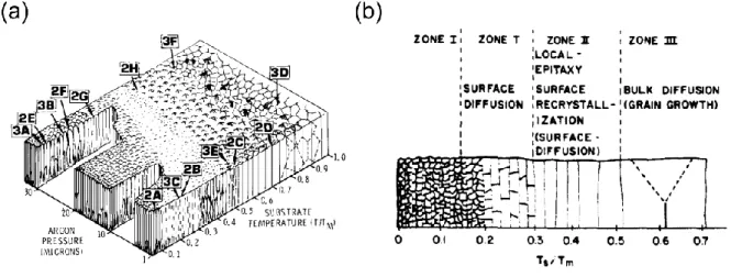
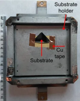
3.1 Sputter Deposition ... 55
3.2 Sample Structure and Patterning ... 61
3.3 Magneto-Optical Kerr Effect ... 67
3.4 Anomalous and Planar Hall Effect ... 72
3.5 Time Resolved Hall Magnetometry under different Atmospheric Conditions ... 74
3.6 Spin-torque Ferromagnetic Resonance ... 77
3.7 Solid Oxide Cell Characterization ... 79
Chapter 4: Effect of H2O on Voltage-induced Co Oxidation in a Pt/Co/GdOx Heterostructure .. 81
4.1: Experimental Methods ... 84
4.2: Probing Water Uptake in GdOx ... 86
4.3: Voltage-induced Co Oxidation in Hydrated and Non-hydrated Pt/Co/GdOx Devices ... 90
4.4: H2 evolution during Voltage-induced Co Oxidation in Pt/Co/GdOx ... 94
4.5: In-situ XAS probe of Co during Voltage-induced Co Oxidation in Pt/Co/GdOx ... 98
Chapter 5: Magneto-ionic Control of Magnetism using a Solid-state Proton Pump ... 100
5.1: Experimental Methods ... 103
5.2: Co Redox through Water Electrolysis ... 105
5.4: Magnetic Response under Short Circuit and Open Circuit... 117
5.5: Electrical Gating of Magnetic Anisotropy at a Heavy-metal/ferromagnet Interface ... 120
5.6 Comparison between Au and Pt Top Electrodes ... 124
Chapter 6: Voltage Gating of Magnetic Damping and Spin-Orbit Torques using Proton ... 126
6.1 Experimental Methods ... 129
6.2 Spin Torque Ferromagnetic Resonance to Probe Voltage Gating of Spin Orbit Torque and Magnetic Damping... 131
Chapter 7: Voltage-induced Magneto-Ionic Effect in Pt/Co/MOx Heterostructure (M= Gd, Y, Zr, and Ta) ... 138
7.1 Experimental Methods ... 141
7.2 Rate of Voltage-Induced Magnetic Modulation at Positive Bias ... 142
7.3 Rate of Voltage-Induced Magnetic Modulation at Negative Bias ... 145
Chapter 8: Room Temperature Reversible Solid Oxide Fuel Cell ... 148
8.1 Experimental Methods ... 150
8.2 Proton Conductivity of GdOx... 152
8.3 Cell Performance and Scalability... 154
8.4 Gating of Magnetism using Built-in Voltage ... 158
Chapter 9: Voltage Gating of Optical Properties ... 161
9.1 Experimental Methods ... 163
9.2 Voltage Gating of Optical Reflectivity in Pt/GdOx/Au Heterostructure ... 164
9.3 Source of Irreversible Optical Change in Pt/GdOx/Au Heterostructure ... 169
9.4 Voltage Gating of GdOx Heterostructures with different Top and Bottom Electrodes .... 172
9.5 Optical Modulation outside Active Region due to Hydrogen Diffusion ... 175
Chapter 10: Electrical Properties of GdOx ... 178
Chapter 11: Summary and Outlook ... 186
11.1 Summary ... 187
11.2 Outlook ... 189
11.2.1 Integration of Hydrogen Storage in Proton Magneto-Ionic Device ... 189
11.2.2 Proton Magneto-Ionics for Memory and Logic Devices ... 190
11.2.3 Proton Magneto-Ionics to Quantify Proton Conductivity in Thin Film Oxides ... 193
1
Chapter 1:
2
1.1 Motivation
As solid state devices continue its path towards miniaturization, there are two important trends to note: (1) interfaces play an increasingly important role in determining material properties1, and (2) the electric field, which is the primary tool by which we control device functions, becomes progressively larger. Simultaneously, the need to dynamically toggle material properties have become more crucial due to limited functionalities and performance imposed by static devices. For instance, in magnetic memory, it is extremely difficult to achieve both thermal stability and low writing power simultaneously because thermal stability implies large energy barrier to magnetic switching, while low writing power implies low energy barrier to magnetic
switching2,3. These are two conflicting requirements which are very difficult to optimize in a static device.
In this thesis, we take advantage of functional interfaces and large electric field in nanoscale devices in order to provide a mechanism by which we can dynamically induce large changes in material properties. We demonstrate dynamic modulation of material properties in thin film devices through solid state proton gating. Proton is used because it has high mobility at room temperature which allows for fast device operation. At the same time, it can induce very large changes in device properties because it disrupts chemical bonding at functional interfaces. In this sense, it captures the best of both worlds in terms of speed of electronic modulation and
magnitude of ionic modulation. The term “magneto-ionic” is used to refer to magnetic-ionic coupling where ions are used to modulate magnetic properties.
3
1.2 Thesis Outline
This thesis is written with the aim to enable a wide audience with little knowledge of magnetism, ionics, or electrochemistry to interpret the new findings.
In chapter 1, we give a preliminary introduction to dynamic modulation of material properties using solid state proton gating.
In chapter 2, we provide some scientific background which is necessary to understanding the results presented in this thesis. The chapter starts off with introduction to magnetism since a large part of the thesis is focused on modulation of magnetic properties. The chapter eventually transitions into introduction to proton conductors and water electro-catalysis because we source protons from water and transport them through an oxide electrolyte to modulate material
properties.
In chapter 3, we provide a detailed overview of the primary experimental techniques used to perform the research in this thesis. The chapter starts off with description of the sample
structures and fabrication steps. This is followed by characterization techniques used to probe the magnetic and electrochemical properties of the samples.
In chapter 4, we present the first experimental evidence that voltage-induced Co oxidation in a Pt/Co/GdOx/Au heterostructure is dominated by water oxidation instead of oxidation by oxygen
ions. The findings represent an important breakthrough in understanding of voltage induced redox in ferromagnet/oxide systems and show that water can play a crucial role in previously observed magneto-ionic effect.
4 In chapter 5, we show for the first time solid state gating of magnetic anisotropy using proton. This discovery allows for 90° toggling of the magnetization in a Pt/Co/GdOx system at
unprecedented speed and cyclability. Proton magneto-ionics also allow for gating of magnetic anisotropy at a metal-metal interface through hydrogen insertion in a heavy metal adjacent to a ferromagnet.
In chapter 6, we demonstrate voltage gating of magnetic damping and spin torques probed using spin-torque ferromagnetic resonance. The results show that a wide range of fundamental
magnetic properties can be gated using ions.
In chapter 7, we compare the rates of voltage-induced magnetic changes in different Pt/Co/MOx
heterostructures, where M is Gd, Y, Zr, or Ta. The results show that speed of magnetic
modulation can change significantly depending on the choice of MOx as the proton conducting
electrolyte.
In chapter 8, we introduce a room temperature reversible solid oxide cell based on hydrogen storage in a thin film oxide. The cell is a miniaturized version of a conventional solid oxide fuel cell, and can be operated like a battery for microelectronics. The finding is important because it shows the applicability of solid-oxide fuel cells for energy storage in microelectronics. In chapter 9, we demonstrate voltage-induced modulation of optical properties in a thin film metal/oxide/metal heterostructure using proton. Fast optical response down to 20ms was achieved with good cyclability. This establishes the wide applicability of voltage-induced protonics to modulate material properties in thin film heterostructures.
In chapter 10, we revisit some electrical properties of GdOx since it is used as the proton
5 In chapter 11, we summarize the findings of the thesis and discuss their impacts. This is followed by a list of recommended future work to fill the remaining gap in our understanding proton gating of material properties. We end by providing a brief outlook for this new field of research.
6
Chapter 2:
7
2.0 Magnetic Hysteresis Loop
The simplest and densest way to describe a magnetic sample is a magnetic hysteresis loop4. A magnetic hysteresis loop is a plot of magnetization vs magnetic field as shown in Figure 2.1(a). In magnetic hysteresis loops, the same magnetic field which is applied does not always produce the same magnetization. The magnetization, M depends not only on the magnetic field which is currently applied, it also depends on its previous state (This is why it is called a “hysteresis” loop).
Figure 2.1. Magnetic hysteresis loop. (a) Easy-axis magnetic hysteresis loop. The coercive
field, HC is typically half the width of the hysteresis loop, while the saturation magnetization, MS
is half the height of the hysteresis loop. (b) A general profile of the applied magnetic field. (c) The measured magnetization corresponding to the magnetic field in (b). (d) The direction of the applied magnetic field and the magnetization. Both are pointing along the y-axis.
To generate a magnetic hysteresis loop, one sweeps the magnetic field and measures the
magnetization at each field according to the profile shown in figure 2.1b. For a sample which is (1) uniformly magnetized in the direction of the magnetic field, and (2) where the magnetization rotates coherently as a single domain (Stoner-Wohlfarth model), the resulting magnetization is shown in figure 2.1c. When we first increase the magnetic field in the +y direction, the magnet
8 starts out pointing in a –y direction (hysteresis from its previous state). When the magnetic field exceeds a critical field, the magnet “abruptly” flips 180º to the positive direction. This critical field is called the coercive field, HC and it quantifies the energy barrier to switch the
magnetization 180º (assuming Stoner-Wohlfarth model). As one increases the magnetic field further in the positive direction, the measured magnetization remains flat. The value at which this magnetization plateaus is called the saturation magnetization, MS. When we next increase the
magnetic field in the –y direction, the magnetization again flips 180º at HC and plateaus at MS
but with a negative sign. If we plot the magnetization versus the magnetic field, we get the magnetic hysteresis loop shown in figure 2.1a.
A magnetic hysteresis loop is measured using a variety of techniques such as magneto-optical Kerr effect, and anomalous Hall effect. In these cases, M is measured indirectly as Kerr rotation or Hall resistance respectively. These will be described in greater details in chapter 3. While we can always extract HC and MS from a magnetic hysteresis loop, the magnetic information is not
limited to the two quantities. For instance, if the magnetic sample is not in a single domain state, then the hysteresis loop can give us qualitative information on the domain configuration. It can also give us information on the magnetic anisotropy depending on which direction the magnetic field is applied in. The details will be discussed in subsequent sections.
In magnetism, there are two kinds of units which are frequently used: cgs (centimeter-gram-second) and SI units. While SI units are more standardized, the magnitude is often too large for thin film magnetism. For this thesis, we will mainly be using cgs units unless stated otherwise.
9
2.1 Magnetic Anisotropy
In an anisotropic system, the magnetization vector tends to point in certain preferred axis because it minimizes its energy. This is called magnetic anisotropy4. The minimum energy axis is called an easy magnetization axis whereas the maximum energy axis is called the hard
magnetization axis. In thin film magnetism, the term “magnetic anisotropy” is typically used in a more specific sense; it represents an energy density, KU needed to rotate the magnetization from
the easy-axis to the hard-axis direction. This value is extremely important because it quantifies the energy barrier which the magnetic moment needs to overcome in order switch180º. In other words, the moment goes through the hard axis as it switches from one direction to the opposite direction4,5.
10
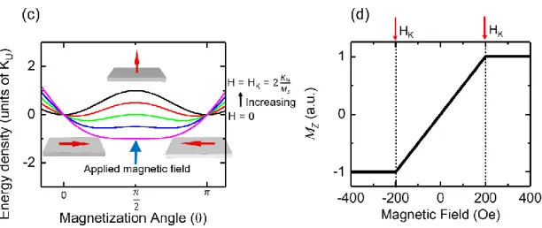
Figure 2.2. Magnetic anisotropy. (a) Energy coordinate of M with the magnetic field applied
along the easy axis in –y direction. (b) Easy axis magnetic hysteresis loop. (c) Energy coordinate of M with the magnetic field applied along the hard axis in +z direction. (d) Hard-axis magnetic hysteresis loop. Adapted from reference5
In figure 2.2, we assumed the easy-axis is the y-axis while the hard axis is the z-axis and we start out with the magnetization pointing in the +y direction. When we apply a magnetic field, H along the easy axis in the -y direction (figure 2.2(a),), we decrease the energy of the –y state while increasing the energy of the +y state. When the energy due to the magnetic field (Zeeman energy) equals the energy barrier arising from the magnetic anisotropy, KU, the magnetization
switches from the +y direction to the -y direction. If one looks at the easy-axis hysteresis loop which shows the y-projection of M (figure 2.2(b)), this happens at the coercive field, HC. If we
instead apply the magnetic field along the hard axis in the +z-direction (figure 2.2(c)), we reduce the energy of the +z state while keeping the ±y state the same. As a result, there is no 180º switching of the magnetization; the magnet simply rotates 90º from +y to +z. If one looks at the hard-axis hysteresis loop (figure 2.2(d)), the z-projection of M gradually increases and saturates at the anisotropy field, HK. Both HC and HK are equal to 2
𝐾𝑈
11 anisotropy is very important in determining the threshold magnetic field to switch or rotate the magnetization.
Magnetic anisotropy arises from two microscopic origins: dipolar interactions and spin-orbit coupling4–7. Dipolar interactions refers to the interaction between magnetic dipoles, and
intuitively, one can think of the dipolar energy being minimized when the one magnetic dipole is aligned along the magnetic field generated by a second magnetic dipole. Dipolar interactions lead to magnetic anisotropy because moments lower their energy when they are aligned along a common axis. In bulk systems, there will be a very large number of these microscopic dipoles; hence to find the stable magnetic configuration, one has to integrate all the individual dipoles to find the minimum dipolar energy of the system. The second microscopic origin of magnetic anisotropy is spin-orbit coupling (SOC). Spin-orbit coupling refers to the coupling between the spin and orbital moments of each atom.
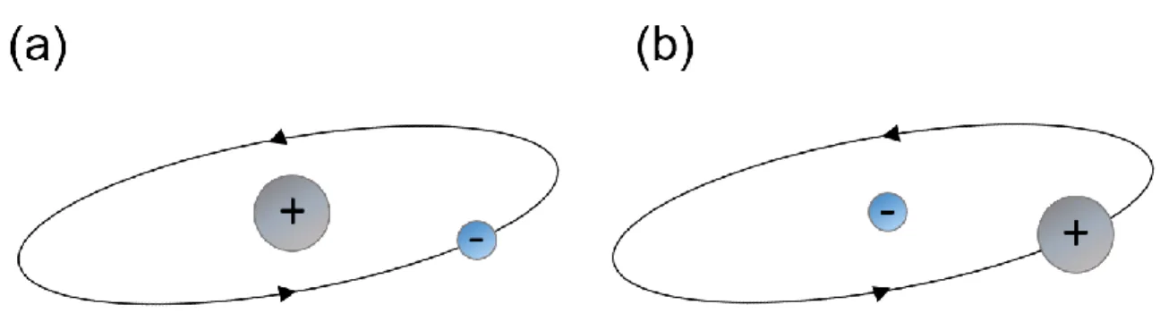
Figure 2.3. Spin orbit coupling. (a) Trajectory of electron from reference frame of the nucleus.
(b) Trajectory of the nucleus from reference frame of the electron
When electron spin orbits the nucleus of an atom, it experiences an effective magnetic field from the nucleus because from the electron’s reference frame, it “sees” the positively charged nucleus orbiting itself (a moving charge generates a magnetic field) (figure 2.3). The magnetic field
12 “generated” from the orbiting nucleus is represented by the orbital moment, L while the electron spin is represented by the spin moment, S. As a result, the energy of spin-orbit coupling is expressed as 𝐸𝑆𝑂 = −𝜉𝐿. 𝑆 where 𝜉 is the coefficient which represents the strength of the
spin-orbit coupling4–7. SOC leads to magnetic anisotropy because it couples the spin moment to the orbital moment. And because the orbital moment is in turn coupled to the crystal lattice, a form of magnetic anisotropy arises where the magnetic moments are stabilized along certain high symmetry axes of the crystal lattice. This form of anisotropy is called magnetocrystalline anisotropy.
In this thesis, we will be focusing on thin film 3d ferromagnet systems where the thickness of the magnetic film is on the order of nm. While the microscopic origins (the two stated above) of magnetic anisotropy are the same for all magnetic systems, in these thin film systems, we classify the magnetic anisotropy into two contributions: a volumetric and a surface contribution. The volumetric contribution, KV (energy per unit volume) is mainly due to shape anisotropy.
This anisotropy refers to the dependence of the magnetization easy axis on the shape of the magnet and it arises due to dipolar interactions. For each shape and magnetization direction, there is a corresponding total dipolar energy, or magnetostatic energy, 𝐸𝑚𝑎𝑔𝑛𝑒𝑡𝑜𝑠𝑡𝑎𝑡𝑖𝑐 which is
given by: 𝐸𝑚𝑎𝑔𝑛𝑒𝑡𝑜𝑠𝑡𝑎𝑡𝑖𝑐 = 1 2𝐻⃗⃗⃗⃗⃗ . 𝑀𝐷 ⃗⃗ (Equation 2.1) 𝐻𝐷 ⃗⃗⃗⃗⃗ = −𝑁𝐷𝑀⃗⃗ (Equation 2.2) Here, 𝐻⃗⃗⃗⃗⃗ is the demagnetizing field, 𝑁𝐷 𝐷 is a geometry-dependent tensor, and 𝑀⃗⃗ is the
magnetization vector. The demagnetizing field 𝐻⃗⃗⃗⃗⃗ , is an effective field experienced by each 𝐷
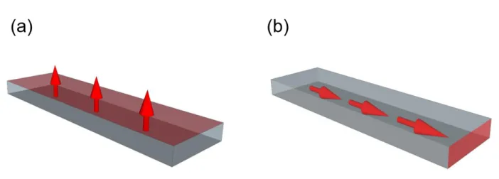
13 anisotropy arises because there is certain magnetization direction relative to the magnet shape where 𝐸𝑚𝑎𝑔𝑛𝑒𝑡𝑜𝑠𝑡𝑎𝑡𝑖𝑐 is minimum. One can further simplify the picture and think of a stable magnetic configuration as one that results in the minimum area of “free” magnetic poles (figure 2.4).
Figure 2.4. Shape anisotropy. The magnetic configuration in (b) results in smaller area of
“free” magnetic poles (shaded in red) in the magnet compared to (a); as a result, (b) has smaller Emagnetostatic.
In an ideal thin film which (1) stretches infinitely in the in-plane directions (x and y-axis) and where (2) the magnetization points out-of-plane (z-axis), 𝐻𝐷 = 4πMS (MS is the saturation
magnetization) (figure 2.5) 4–7. This field points opposite to the out-of-plane magnetization, resulting in 𝐸𝑚𝑎𝑔𝑛𝑒𝑡𝑜𝑠𝑡𝑎𝑡𝑖𝑐 of 2πMS2. If the magnetization points in any in-plane direction, the
resulting 𝐸𝑚𝑎𝑔𝑛𝑒𝑡𝑜𝑠𝑡𝑎𝑡𝑖𝑐 is 0. Hence, for a thin film magnet, assuming a negative convention for in-plane anisotropy (magnet prefers to point in-plane), the volumetric magnetic anisotropy, KV =
14
Figure 2.5. Demagnetizing Field. Cross section of a thin film magnet showing the directions of
the magnetic moment and the demagnetizing field.
For practical applications, it is the out-of-plane magnetic configuration which is desired in order to achieve the highest memory density2,8–11. Another commonly used term for out-of-plane
magnetic anisotropy is perpendicular magnetic anisotropy (PMA). Fortunately, in a thin film system, the surface magnetic anisotropy, KS (energy per unit area) tends to favor PMA.
Generally speaking, in thin film ferromagnet with broken inversion symmetry, there is splitting in degeneracy of the different orbitals (figure 2.6). Due to electrostatic interactions, these lower energy orbitals tend to have an out-of-plane anisotropy.
Figure 2.6. Surface magnetic anisotropy. Schematic illustration of splitting of degeneracy in
15 Because PMA is generated by filling bands with out-of-plane orbital anisotropy, the position of the fermi level is very important. One way to tune the fermi level is through hybridization with heavy metals at the ferromagnetic interface. For instance, it has been known for many years that large PMA exists in in Co/Pt and Co/Pd multilayers13,14 due to hybridization of the Co 3d orbitals with the 5d and 4d orbitals of Pt and Pd respectively15–19. This hybridization tunes the fermi level such that the out-of-plane orbitals are maximally filled and provides large spin-orbit coupling from the Pt and Pd atoms. This hybridization is localized at the Co/Pt or Co/Pd interface and, for a Co thickness of at least a few monolayers, this interface constitutes the majority of the PMA across the entire Co film (figure 2.7)17.
Figure 2.7. Orbital moment near the Co/Pt interface. The perpendicular magnetic anisotropy
is largest closest to the Co/Pt interface. Adapted with permission from reference17.
More recently, it has been shown that hybridization between the s-p orbitals of the oxygen atom and dz-orbitals of a 3d ferromagnetic metals such as Co and Fe can also stabilize PMA20,21. This
16 position of the oxidation front is very important in determining the strength of the PMA. By starting out with a Pt/Co/Al trilayer structure and subjecting the top Al layer to different duration of plasma oxidation front, Manchon et al found that the largest PMA is obtained when the
oxidation front is right at the Co/Al interface, where the structure is exactly Pt/Co/AlOx(figure
2.8)22,23. When the Al is underoxidized, the Co magnetization points in-plane whereas if it is overoxidized (Pt/Co/CoO/AlOx), the PMA starts to decrease again.
Figure 2.8. PMA as function of interfacial oxidation. (a) Anisotropy field, Han as a function of
plasma oxidation time of the Pt/Co/Al trilayer structure. (b) Hall effect magnetic hysteresis loops corresponding to different plasma oxidation times. Largest PMA is obtained when the oxidation front is exactly at the Co/Al interface. Adapted with permission from reference22.
The total magnetic anisotropy, KU is given by the sum of the surface (KS) and volumetric
17 𝐾𝑈 = 𝐾𝑉 +𝐾𝑆
𝑡 Equation 2.3
Where 𝑡 is the thickness of the ferromagnetic film. Due to the competition between KS and KV,
there is a critical thickness below which one gets PMA and above which one gets an in-plane magnetic state. This is shown in figure 2.9, where the authors plotted Keff *tCo against tCo (the
symbol Keff is used in place of KU, Co is the magnetic material). Note that the intercept is 2KS
because there are two surfaces where KS is present.
Figure 2.9. Keff*t versus t for a Pd/Co multilayers. Keff*t corresponds to in-plane magnetic
anisotropy while Keff*t > 0 corresponds to perpendicular magnetic anisotropy. Adapted with
permission from reference16.
While we have so far focused on surface anisotropy arising from interfacial hybridization in a static structure, it has also been known that gas adsorption on ultra-thin magnetic films can alter magnetic anisotropy. One of the most studied gas is hydrogen, H2 which can either physiosorb as
molecules or chemisorb on metallic thin film after splitting into individual H atom24–31. Mankey
18 enhancing that of Fe24. According to the authors, this is because the majority sub-band is nearly filled in Co whereas it is only partially filled in Fe; as a result, when electrons are added due to hybridization with hydrogen, they are added to the minority band in Co and majority sub-band in Fe. This changes the Co and Fe magnetizations in opposite directions. Valvidares et al have found through magneto-optical Kerr imaging that adsorption of hydrogen on a Pt(111) substrate before the deposition of a thin Co layer (t < 1.3nm) decreases the PMA significantly25. Using ab-initio calculations, they found a large reduction in magnet moments of the Co, which in turn reduces the magnetic moment in Pt induced by proximity effect. As Pt atoms constitute the largest source of spin-orbit-coupling, this results in a significant reduction in the PMA. Similarly, Munbodh et al have found that hydrogen absorption in Co/Pd multilayers decreases both the magnetic moment and PMA in the structure due to decreased induced moments in the Pd layer26. Unlike Co heterostructures, Sander et al instead found that exposure of Ni/Cu(001) to hydrogen induces PMA, and by cycling the hydrogen partial pressure they were able to cycle the
magnetization between in-plane and out-of-plane state reversibly (figure 2.10)27. In the case of Ni, the authors attribute the change in magnetic anisotropy mainly to tetragonal distortion in the Ni crystal structure.
19
Figure 2.10. Reversible hydrogen gas induced magnetization switching. Polar
magneto-optical Kerr signal (proportional to out of plane magnetization) of a Ni/Cu(001) thin film structure as a function of partial pressure of hydrogen. Inset shows the direction of the magnetization. Adapted with permission from reference27.
20
2.2 Magnetization Dynamics and Spin
Current
So far, we have pictured magnetization as moments which are aligned in a static configuration along a magnetic field. However, magnetic moments undergo a precessional motion when subjected to the slightest torque exerted by either a magnetic field or a spin current.
Magnetization dynamics is usually modelled by the Landau-Lifshiftz-Gilbert (LLG) equation which is given by:
𝜕𝑚
𝜕𝑡 = −𝛾𝑚 × 𝐻𝑒𝑓𝑓+ 𝛼𝑚 × 𝜕𝑚
𝜕𝑡 Equation 2.4
Where 𝑚 is the magnetic moment vector, 𝜕𝑚
𝜕𝑡 is evolution of the magnetic moment as a function
of time, and 𝐻𝑒𝑓𝑓 is an effective field which includes contribution from the demagnetizing field, interfacial anisotropy, and the applied field, H. 𝛾 is the gyromagnetic ratio and 𝛼 is the Gilbert damping parameter. The first term on the right (−𝛾𝑚 × 𝐻𝑒𝑓𝑓) represents the field-like torque which causes the magnetization to precess around 𝐻𝑒𝑓𝑓 while the second term on the right is the
damping-like torque (𝛼𝑚 ×𝜕𝑚
𝜕𝑡) which causes the magnetic moment to gradually “dampens”
21
Figure 2.11. Magnetization dynamics according to the LLG equation. Adapted from
reference32.
The original LLG equation was later modified to include spin-current induced torques
𝜕𝑚 𝜕𝑡 = −𝛾𝑚 × 𝐻𝑒𝑓𝑓 + 𝛼𝑚 × 𝜕𝑚 𝜕𝑡 + 𝜏𝐹𝐿 𝑠×𝑚 |(𝑠×𝑚)|+ 𝜏𝐷𝐿 𝑚×(𝑠×𝑚) |𝑚×(𝑠×𝑚)| Equation 2.5
Where 𝜏𝐹𝐿 and 𝜏𝐷𝐿 are magnitudes of spin-current induced field-like and damping-like torques, and s is the polarization of the spin current. Here, the third 𝜏𝐹𝐿 𝑠×𝑚
|(𝑠×𝑚)| and the fourth
(𝜏𝐷𝐿 𝑚×(𝑠×𝑚)
|𝑚×(𝑠×𝑚)|) terms are called the spin current induced field-like and damping-like
(Slonczewski) torques respectively because they have the same symmetry as the corresponding field induced field-like and damping like torques. In this case, the spin current provides an effective exchange field along the direction of its spin polarization. The third term drives the moment to precess around this spin polarization direction while the fourth term drives the
moment to “dampen” towards the spin polarization direction. One way to generate spin current is using the spin Hall effect where spin-orbit coupling in heavy metals drives spin current to flow in tranverse direction to the charge curren (figure 2.12)33–35 .
22
Figure 2.12. Spin current induced by the spin Hall effect in Pt layer. The spin current
injected into the CoFe ferromagnetic layer generates a torque to drive magnetization dynamics or switching. In this schematic, the charge current is along the x-axis, the spin current is along the z-axis, and the spin polarization is along the y-axis. There is an exchange field due to the spin current along the spin polarization direction. Adapted with permission from reference36.
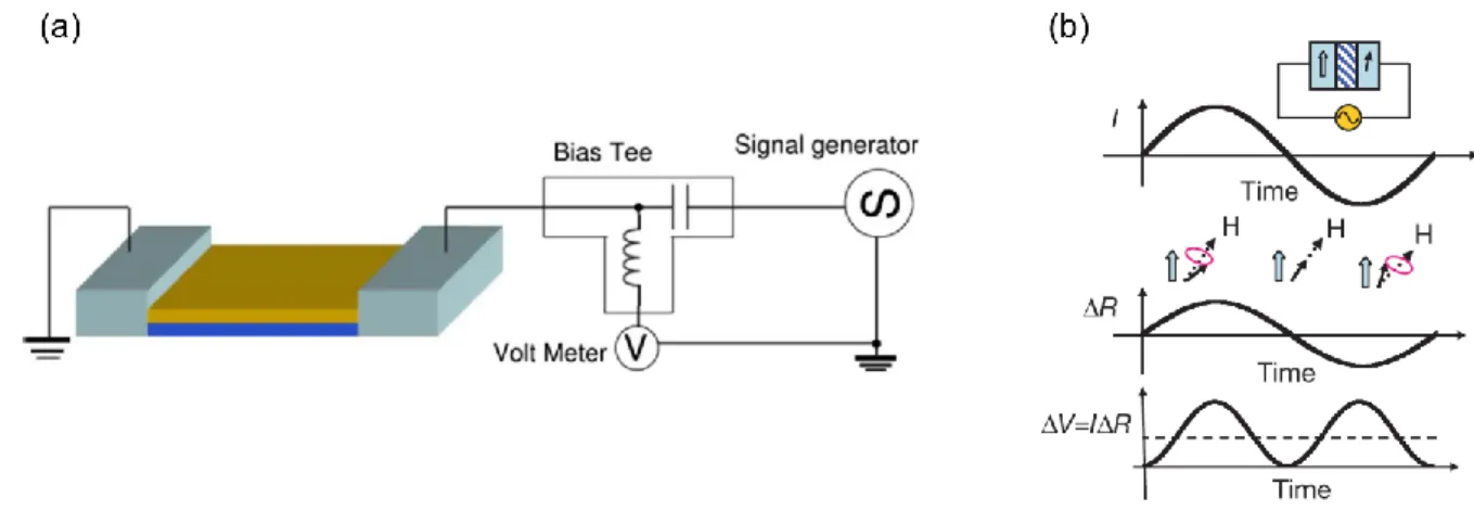
Magnetization dynamics can be characterized using ferromagnetic resonance (FMR). In
conventional FMR, a magnetic field at high frequency is applied to a magnetic sample to provide a torque (equation 2.4) which drives the moments to precess. Simultaneously, the absorption of microwave radiation by the magnetic sample is measured in a microwave cavity. At resonance, there will maximum absorption of radiation by the sample. The resonance frequency (or field) then provides quantitative information about the 𝐻𝑒𝑓𝑓 experienced by the sample while the width of the absorption peak is proportional to its damping parameters.
In this thesis, we instead rely on a variation of conventional FMR called spin-torque FMR (ST-FMR) to characterize the magnetic properties of the magnetic sample37–40. A heavy metal such as Ta or Pt is used to generate spin current using the spin Hall effect39. The generated spin current is then used to drive magnetization precession in an adjacent ferromagnetic layer. The precession of the magnetic layer manifests itself electrically as a change in DC resistance through
23 magnetoresistance, which can be measured as a mixing voltage(figure 2.13). A detailed
description of the method and analysis will be given in chapter 6.
Figure 2.13. Spin-torque ferromagnetic resonance (ST-FMR). (a) Schematic of the ST-FMR
measurement configuration. (b) Current induced change in magnetoresistance (ref. spin torque diode effect). Adapted with permission from references38,39.
24
2.3 Magneto-Electric and Magneto-Ionic
Effects
In magnetic memory, the ultimate goal is to have high memory density, low writing power, and high thermal stability2. To achieve high memory density, the size of magnetic bit can be made
smaller. However smaller bits lead to degradation of the thermal stability because the energy barrier to flip the magnetization is given by ∆𝐸 = 𝐾𝑢𝑉, where V is the volume of the magnetic bit. ∆𝐸 has to be at least 60kT in order to have stable recording for more than 10 years (k is the Boltzmann’s constant). One may compensate for this size reduction by increasing the magnetic anisotropy, 𝐾𝑢 but as discussed in the previous section (chapter 2.1) the magnetic field, 𝐻𝑐
required to switch the magnetization is proportional to 𝐾𝑢. As a result, the total writing power also increases. This challenge in achieving high memory density, low writing power, and high thermal stability simultaneously in magnetic memory is called the trilemma.
One approach to overcoming the trilemma is to utilize a dynamic system where we reduce the switching barrier temporarily during the writing operation. This can be done most effectively using a gate voltage, and one of the mechanisms which allows for such modulation is the magneto-electric effect. Magneto-electric effect refers to a wide range of phenomena which allow for control of magnetization using an electric field. Magneto-electric phenomena can be broadly classified into three main classes of materials: dilute magnetic semiconductors (DMS), multiferroic materials, and ultra-thin metallic ferromagnet/oxide bilayers. The magneto-electric coupling can be an intrinsic feature of the single phase material, or it can be coupled in
25 Dilute magnetic semiconductors (DMS) are semiconductors which exhibit magnetic properties due to low level doping by ferromagnetic metals such as Mn41,42. The most studied of these DMS
is Mn-doped InGaAs which exhibits ferromagnetic properties due to hole-mediated interaction41–
44. With decreasing hole concentration, a super-exchange interaction which favors
antiferromagnetic configuration starts to dominate; as a result an electric field can reversibly change the magnetic properties by changing the hole concentration through charge injection43–45. This was first demonstrated by Chiba et al where they electrically gate the magnetic moment of (In,Mn)As through modulation of its Curie temperature (figure 2.14)44. However, the major problems with these systems are their extremely low Curie temperature (typically <50K) and the complex fabrication steps to induce the ferromagnetism.
Multiferroics, on the other hand, are materials which exhibit magnetic and ferroelectric orders simultaneously46. All of these materials have perovskite structures. In these materials, non-zero magneto-electric coupling coefficient can arise from structural asymmetry; as a result, an electric field can induce a change in magnetization and vice versa. Besides magneto-electric coupling in a single phase system with non-zero magneto-electric coefficient, magneto-electric coupling can also be engineered in heterogeneous ferroic media47–50. In this case, exchange or elastic coupling between a ferroelectric and ferromagnetic material can allow for electric field control of
magnetization. Figure 2.15 shows an example of such system, where magnetic CoFe2O4
nanopillars are embedded with out-of-plane epitaxy in a ferroelectric BaTiO3 medium. When an
electric field is applied, the resulting strain in the ferroelectric BaTiO3 is imparted to the
CoFe2O4 nanopillars, causing a change in its magnetization48,49. While these systems have very
26 growth requirements (substrate epitaxy, growth temperature etc.) which are incompatible with current CMOS processes.
Figure 2.14. Electric field control of ferromagnetism in a dilute magnetic semiconductor.
(a) Schematic of device operation of a magnetic (In,Mn)As during electrical gating. (b) Hall hysteresis loops of the (In,Mn)As at different gate voltages. Adapted with permission from reference44.
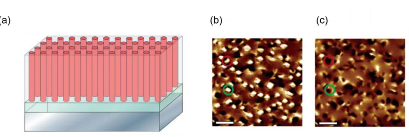
Figure 2.15. Magneto-electric coupling in a heterogeneous multiferroic system. (a)
Schematic of magnetic CoFe2O4 (CFO) nanopillars embedded in a ferroelectric BaTiO3
(BTO)matrix. (b)-(c) Magnetic force microscope images of the CFO-BTO composite before and after electrical poling at +12V. The region in red circle represents magnetization reversal upon electrical poling. The green circle represents multi-domain formation. Adapted with permission from references48,49.
27 The third class of materials where magneto-electric coupling has been observed is ultra-thin metallic ferromagnet/ oxide bilayer systems12,51,52. In these devices, the ferromagnet needs to be
thin (<1nm) due to Coulombic screening in metals. Electric field-induced magnetic changes in these materials has been attributed to a few factors: (1) spin-dependent screening of the electric field can induce a net surface magnetization in an ultra-thin ferromagnet53. (2) electric field can also lead to different occupation of the 3d orbitals at the surface layer of the ferromagnet; this in turn changes the magnetic anisotropy54. (3) Besides changing the orbital occupation, it was also
proposed that an electric field directly changes the band structure of the ferromagnet and hence the magnetic anisotropy55. The magneto-electric efficiency that has been predicted and
demonstrated in these ultra-thin ferromagnet is on the order of ~10 fJ/Vm. This value however is too small for practical device applications. To put the value into context, an electric field of ~1MV/cm only induces a magnetic anisotropy change of a few percent in thermally stable ferromagnetic devices. Figure 2.16 shows an example of an ultra-thin film ferromagnet/oxide magnetoelectric device and its operation.
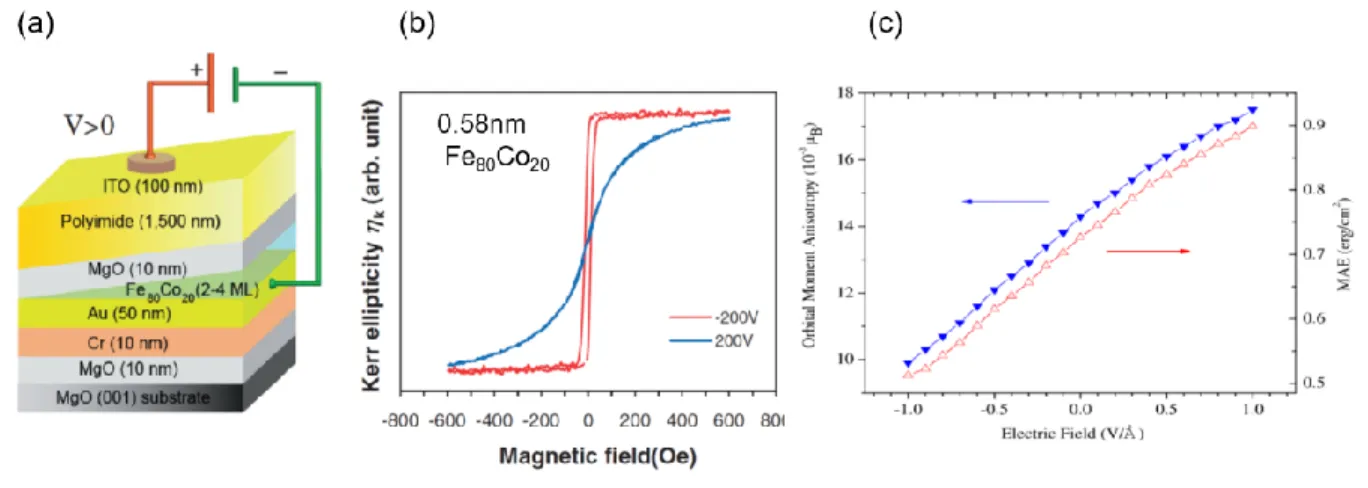
Figure 2.16. Magneto-electric effect in ultra-thin film ferromagnet/oxide device. (a)
Magneto-optical Kerr effect hysteresis loops of the Fe80Co20 magnetic film in (a) at V = ±200V.
(c) Simulated change in orbital magnetic anisotropy and magnetic anisotropy energy (MAE) as a function of electric field for a free standing 15 monolayer thick Fe (001) film. Adapted with permission from reference56,57.
28 Besides magneto-electric effect, another promising route to effective voltage control of
magnetism is through ionic modulation of magnetic interfaces58–65. This approach relies on
voltage-induced ionic migration and electrochemistry to modulate magnetic properties ranging from magnetic anisotropy to spin-orbit torques. One example of magneto-ionic control of
magnetism is reversible oxidation and reduction of the Co ferromagnet layer in a Pt/Co/GdOx/Au
heterostructure (figure 2.17). The redox of the Co layer is confirmed by electron energy loss spectroscocpy (EELS) and x-ray magnetic circular dichroism (XMCD) analyses60,61. While the
voltage-induced redox process is originally confined to the electrode edge, further optimizations enabled uniform redox across the entire device region (figure 2.14). Oxygen-based magneto-ionics were also demonstrated in Co/SrCoOx66,67, Co/HfOx68, Co/ZnO69, and CoFeB/MgOx
systems70.
Figure 2.17. Magneto-ionic control of magnetism through voltage-induced redox of Co. (a)
Schematic of a Pt/Co(0.9nm)/GdOx/Au device. (b) EELS spectrum of the normalized O-K edge
count as a function gate voltage (Ubias). (c) Polar magneto-optical Kerr effect hysteresis loop of
29 Besides oxygen-ion, Group I ions like lithium ions and protons have also been used to induce changes in magnetic properties67,71–73. For instance, Zhang et al have demonstrated large changes
in magnetic moments by reversible intercalation of lithium ions in spinel structures like
Fe2O3(figure 2.18)73. These experiments are done in a battery-like configuration with the spinel
structure acting as the cathode inside a liquid electrolyte. Similarly, proton-induced modulation of magnetic properties have also been demonstrated by Nan et al in an acidic solution through reversible absorption and desorption of hydrogen on an ultra-thin Co film74. More recently, Lu et
al have demonstrated that hydrogen and oxygen-induced phase transformation in SrCoOx can
lead to reversible transition between a paramagnetic, ferromagnetic and antiferromagnetic state (figure 2.18b)67.
Magneto-ionic gating of magnetism has garnered great interest in recent years due to the extremely large magneto-electric efficiency that can achieved, which is on the order of
~5000fJ/Vm61. This allows its implementation in devices to be more practical in terms of power saving. However, there are a few major issues which remain to be addressed. For oxygen-ion gating, it has been shown that irreversible structural and chemical degradation of the target ferromagnet always accompany the magnetic property changes62. In addition, while oxidation of the ferromagnet has indeed been observed through TEM-EELS studies, there is a lack of
understanding on the mechanism of oxidation and the source of oxidant. For lithium ion gating, the major problem remains the incompatibility of most Group I ions with CMOS processing due to formation of traps and defects in Si or SiO275. The exception to this is proton, where it is
relatively innocuous in its standard state. While proton gating is promising, it has only been demonstrated using liquid electrolyte. This thesis henceforth aims to fill the gap in understanding
30 of oxygen-ion gating of magnetic properties, and to demonstrate for the first time proton gating of magnetic properties in an all-solid-state device.
Figure 2.18: Magneto-ionic control of magnetism using lithium ion and proton. (a)
Reversible change in magnetization of Fe through intercalation of Li in Fe2O3 spinel structure.
(b) Reversible insertion of protons and oxygen ions in SrCoO2.5 to change the magnetization
between antiferromagnetic, paramagnetic, and ferromagnetic states. Adapted with permission from references67,73.
31
2.4 Solid Oxide Fuel and Electrolyzer cell
The simplest fuel cell produces power from reaction of H2 and O2 to produce H2O, while an
electrolyzer cell produces H2 fuel and O2 from electrolysis of H2O76–78. Both cells share the same
device structure; whether it is a fuel or electrolyzer cell depends on the mode of operation. A solid oxide cell, unlike conventional liquid electrolyte cells, uses a solid oxide electrolyte such as Yttria-stabilized Zirconia (YSZ); as a result they are typically operated at high temperature (> 700C). A solid oxide cell can be further classified into a proton conducting oxide cell or an oxygen-ion conducting oxide cell79,80. The main difference lies in the type of ions conducted across the oxide; in the former case, it is a proton which gets transported, while in the latter case, it is an oxygen ion. Figure 2.16 shows schematics of a proton-conducting and oxygen-ion
conducting solid oxide cell respectively run in electrolysis mode. The cells consist of two electrodes sandwiching a solid oxide electrolyte layer. One electrode is the anode, where oxidation takes place, while the other is the cathode where reduction takes place. Because the anode and cathode assignment can change depending on operations modes, the electrodes facing O2 and H2 are also known as the air and hydrogen electrode respectively79,80.
32
Figure 2.19. Solid oxide cell in electrolysis mode. (a) Proton conducting solid oxide cell. (b)
Oxygen-ion conducting solid oxide cell.
During operation of a proton conducting electrolyzer cell, a positive bias larger than the thermodynamic potential of water splitting is applied to the air electrode (anode), which splits water to produce proton and oxygen gas. The proton, 𝐻+ then gets transported across the oxide due to the applied electric field, where it gets reduced at the hydrogen electrode (cathode) to produce hydrogen gas. The reactions are shown below:
Proton conducting oxide electrolyzer cell
Anode: 2𝐻2𝑂 → 𝑂2+ 4𝐻++ 4𝑒− Equation 2.6 Cathode: 4𝐻++ 4𝑒− → 2𝐻
33 For an oxygen-ion conducting solid oxide electrolyzer cell, the reaction starts at the hydrogen electrode (cathode), where a negative bias splits water to produce oxygen ions and hydrogen gas. The oxygen ions are driven by the electric field to the air electrode (anode), where it gets
oxidized to oxygen gas.
Oxygen-ion conducting oxide electrolyzer cell
Cathode: 2𝐻2𝑂 + 4𝑒− → 2𝐻2+ 2𝑂2− Equation 2.8 Anode: 2𝑂2−→ 𝑂
2+ 4𝑒− Equation 2.9
Equation 2.6 and 2.9 are known as the oxygen evolution reaction (OER) while equation 2.7 and 2.8 are known as the hydrogen evolution reaction (HER) (More discussion in Chapter 2.6). The operation of a fuel cell is essentially an electrolyzer cell run in reverse mode; for instance, in figure 2.19(a), hydrogen gas would be oxidized to H+, which gets transported to the cathode where it recombines with O2 gas to form H2O.
Some examples of well-known proton conducting oxide electrolyte include barium cerate, BaCeO3 (BCO) and barium zirconate, BaZrO3 (BZO) while examples of oxygen-ion conducting
oxide electrolyte include yttria-stabilized zirconia, YxZr1-xO2 (YSZ) and gadolinium-doped ceria,
Ce1-GdxO2 (GDC) 81–83. Common air electrodes include lanthanum strontium manganite, La 1-xSrxMnO3 (LSMO) while hydrogen electrodes include ceramic composites such as
Ni-YSZ84,85. A more extensive discussion of solid oxide cell electrodes will be given in Chapter 2.6 to 2.7.
One figure of merit to characterize performance in a solid oxide fuel cell is power density. It is measured by sourcing current from a fuel cell and measuring the resulting voltage at a specific temperature and partial pressure of H2 fuel. This is repeated for increasing current values to get
34 the power density curve. Power density depends on a wide range of factors such as overpotential (discussed below), number of active sites on the electrode catalyst, and gas transport of the reactants to the active sites. Figure 2.20(a) shows an example of a power density curve for a solid oxide fuel cell with 0.3mm thick YSZ. An analogous plot can also be generated for an
electrolyzer cell (Figure 2.20(b)); in this case, low voltage and power are desired for operation of the cell.
Figure 2.20. Performance of a solid oxide fuel cell and electrolyzer cell. (a) Exemplary power
density curve of a fuel cell. (b) Analogous performance plot for an electrolyzer cell. Adapted with permission from reference78,86
In an electrolyzer cell, the goal is to maximize the rate of H2 production from water splitting at
minimum potential. For a fuel cell, the goal is to achieve highest power output at maximum potential from hydrogen-oxygen recombination to form water. In both cases, the maximum (fuel cell) and minimum (electrolyzer cell) achievable voltage is the thermodynamic potential, which is 1.23V for H2O at standard conditions. To characterize deviations from this thermodynamic
35 additional volts above the thermodynamic potential is required to split water in an electolyzer cell, or how many volts less than the thermodynamic potential that we can extract from water generation in a fuel cell. Studies of electrolyte and electrode materials are intended to minimize this overpotential, as it represents a loss. There are in general three types of overpotentials: activation overpotential, ohmic overpotential, and concentration overpotential. Activation overpotential arises because, the kinetics of charge transfer at thermodynamic potential is very slow; as a result an additional voltage is required to drive this reaction in the anodic or cathodic direction. Ohmic overpotential arises from ohmic loss and is mitigated by reducing the overall resistance of the cell. Concentration overpotential arises from limited kinetics of the mass transport of either the reactants to the active sites or products from the active sites. For solid oxide cells, activation and concentration overpotential are primarily minimized through
optimization of the electrodes. For ohmic overpotential, the overall resistance is reduced through optimization of the electrodes, electrolyte, and also the electrode/electrolyte interface. The net voltage, 𝑉 that can be extracted from a fuel cell after accounting for all sources of overpotential is given in equation 2.10. Similarly, the voltage that is needed in an electrolyzer cell after accounting for all sources of overpotential is given in equation 2.11. Another term which is commonly used in place of overpotential is polarization loss.
𝑉 = 𝐸𝑜− 𝜂𝑜ℎ𝑚𝑖𝑐− 𝜂𝑎𝑐𝑡𝑖𝑣− 𝜂𝑐𝑜𝑛𝑐 Equation 2.10 𝑉 = 𝐸𝑜+ 𝜂𝑜ℎ𝑚𝑖𝑐+ 𝜂𝑎𝑐𝑡𝑖𝑣+ 𝜂𝑐𝑜𝑛𝑐 Equation 2.11
Here, 𝜂𝑜ℎ𝑚𝑖𝑐 , 𝜂𝑎𝑐𝑡𝑖𝑣, and 𝜂𝑐𝑜𝑛𝑐 are the ohmic, activation and concentration overpotentials
36
2.5 Solid Oxide Proton Conductors
Solid oxide proton conductors have mainly been developed as electrolytes for fuel cell applications. The main motivation for choosing an electrolyte with the largest proton
conductivity is to reduce the ohmic overpotential and to maximize the power density that can be extracted from the fuel cell.
Proton conduction can in general be classified into two broad categories: one based on the Grotthuss mechanism and another based on the vehicle mechanism81,82,87. In Grothuss
mechanism, proton migration is achieved by proton “hopping” between oxygen host lattice sites, and the net transfer of proton depends crucially on factors like lattice dynamics and distance between the oxygen host atoms. If proton migration only depends on proton “hopping” between static host oxygen atoms, the conductivity should increase with decreasing distance between neighboring sites. However, in many cases, this is completely opposite; structures with larger oxygen-oxygen distance exhibits larger proton conductivity. The reason for this is the transfer of proton involves cooperative movement of neighboring oxygen atoms which get closer/further apart momentarily due to lattice vibrations. This allows proton to break and reform hydrogen bonds with neighboring atoms, resulting in a net migration of proton. The lattice dynamics of oxygen atoms is crucial for hydrogen bond breaking; and for short stiff bonds where the oxygen atoms approximate a static lattice, the proton remains essentially “trapped” in a symmetrical bond. In general, bulk proton conductivity (non-grain boundary) of solid-oxide proton conductors can be attributed to the Grotthuss mechanism.
37
Figure 2.21. Coordinates of proton conduction through Grotthuss mechanism. (a)
Conduction through proton “hopping” between static oxygen lattice atoms. (b) Conduction involving both proton “hopping” and oxygen atom lattice vibration. (c) Conduction involving only oxygen atom lattice vibration to break hydrogen bonds. Adapted with permission from reference88.
The second type of proton conduction mechanism is the vehicle mechanism, where proton migration through the electrolyte is a mediated by a vehicle, such as a H2O molecule. In this
case, the rate of diffusion of the vehicle can play a crucial role in determining the overall proton conductivity (in addition to the rate hydrogen bond breaking). The vehicle mechanism dominates in a liquid-like environment where molecules can easily diffuse around, unlike a solid oxide lattice where the atoms are relatively rigid.
The most studied solid oxide proton conductors are the perovskite-structure oxides such as doped BaCeO3 and BaZrO379,89–91. Other well-known proton conductors include phosphates like LaPO4,
38 rare earth oxides such as Gd2O3 , orthoniobates and orthotantalates such as LaNbO492–94. A
compilation of their conductivity values are shown in figure 2.22.
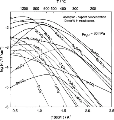
Figure 2.22. Proton conductivities of different oxides. Adapted with permission from
reference82.
In almost all proton conducting oxides, acceptor doping is required to generate oxygen vacancies, and these vacancies in turn absorb water to form hydroxide defect according to the reaction:
𝐻2𝑂 + 𝑂𝑂𝑥+ 𝑉𝑂∙∙ → 2𝑂𝐻𝑂∙ Equation 2.12
Here 𝑂𝑂𝑥 represents an oxygen ion on a normal oxygen site, 𝑉𝑂∙∙ an oxygen vacancy with net double positive charge relative to the normally occupied lattice site, and 𝑂𝐻𝑂∙ a singly positively
39 charged proton localized around an oxygen ion sitting on a normal oxygen site. These localized protons form the charge carriers, and because proton conductivity (𝜎) is a function of both the concentration of carriers (𝑛), charge (𝑞) and mobility (𝜇), according to the reaction 𝜎 = 𝑛𝑞𝜇, the larger the amount of dissolved water, the larger is the proton conductivity. While large acceptor doping can increase the concentration of carriers, excess doping will lead to lattice reordering and strain effects, which in turn reduce the mobility, 𝜇. In addition, not all oxygen vacancies that are created by doping will react with water to form hydroxide defects according to equation 2.12. This will depend on the enthalpy of dissolution of water in the oxide. In general, the more
exothermic is the enthalpy, the more water can be dissolved in the oxide. For rare earth oxides, higher stability of oxide leads to larger exothermic enthalpy and hence dissolution of water in the oxide according to equation 2.12. This is counterintuitive because it is the least stable rare earth oxides (La2O3) that is most reactive with water to form hydroxide. On the other hand, for
perovskites such as BaZrO3 and BaCeO3, it is the larger basicity that has been attributed to larger
dissolution of water. In these perovskites, their stability is inversely related to their capacity for dissolution of water. For instance, in the case of BaCeO3, it decomposes to Ba(OH)2 and CeO2 at
40
Figure 2.23. Rotation and proton transfer in a perovskite structure. Adapted with
permission from reference82
For the mobility of proton carriers, the trend is more complicated, as it depends on a series of steps such as rotation around the oxygen host atom and proton transfer (involving hydrogen-bond breaking). There are however some general trends: (1) the reduction in symmetry of the lattice reduces the mobility, such as in SrCeO3, because dissimilar environment for proton
hopping reduces net permutations of ways to get from one site to another96. (2) For rare earth oxides, mobility decreases as the lattice parameter of the lattice decreases. So far, the best known solid oxide proton conductors are BaCeO3 and BaZrO3, with proton conductivities between 10 -1S/cm and 10-3S/cm at ~700C. However, as mentioned, BaCeO
3 is not stable under high water
partial pressure. BaZrO3 on the other hand, cannot be sintered well which leads to large volume
of grain boundaries and higher resistance. A lot of research effort is hence focused on improving the stability of BCO and sinterability of BZO through doping and special fabrication techniques. Besides proton conductivity through grains, there has also been evidence of proton conductivity through surface and grain boundaries in some nanocrystalline materials. In these systems, there is water uptake in the grain boundaries and surface, and because the volumetric ratio of both
41 components to grain is very large, this form of proton conduction can dominate97–99. One
disadvantage of such proton conductors is increasing temperature will decrease the proton conductivity as water vaporizes, as shown for nanocrystalline ceria in figure 2.24(a) and nanocrystalline YSZ in figure 2.24(b). At higher temperature, the ionic conductivity is dominated by another charge carrier, such as oxygen vacancies. In addition, the difference in ionic conductivities in wet and dry atmospheres can be a few orders of magnitude at room temperature.
Figure 2.24. Proton conductivity of nanocrystalline oxide. (a) Conductivity plot of
nanocrystalline ceria. (b) Conductivity plot of nanocrystalline YSZ. Ionic conduction in both oxides are dominated by proton conduction through water. Adapter with permission from references98,99.
For this thesis, there are some differences between the devices studied and majority of solid oxide cells in literature. While there are many proton conducting oxides that have been
42 investigated at intermediate temperatures (~500C to 700C), almost none has been studied at room temperature (25C). For voltage-gating of functional interfaces using protons, we are mainly only interested in operation at low temperatures (<100ºC). From extrapolation of the
intermediate temperature data, we can already observe significantly different trends and
candidates from what were generally known as “good” proton conductors. Another significant difference between conventional studies and this thesis is the dimension of the device. The thinnest proton conducting electrolyte that has been studied for fuel and electrolyzer cells is a few hundred nm; this thickness is constrained by mechanical strength of the electrolyte
membrane when subjected to high partial pressure of reactant gases. However, the thickness of the proton conductor used in this thesis is down to 4nm, which is >100x smaller. At such dimension, the electric field is extremely large (1-10MV/cm) and can have drastic, non-linear effect on the motion of ions, as seen in many memristive devices100. Figure 2.25 shows some
driving forces which may be present under such large fields.
Figure 2.25. Driving forces for ionic migration in memristive devices under large fields. (a)
Driving force due to drift. (b) Driving force due to electromigration (c) Driving force due to concentration gradient. (d) Driving force due to temperature gradient. Adapted with permission from reference100.
43 Finally, for voltage gating of functional interfaces using protons, the primary figure of merit for fast device response is proton mobility rather than proton conductivity as long as there is sufficient concentration of proton to alter the interfaces. While oxides with large proton
conductivities generally have large proton mobilities, this is not always the case. One example of this is BaTiO3, where the proton conductivity is very low due to low solubility of hydroxide
44
2.6 Water Electro-Catalysis
While electrolyte conducts ions across a cell, water splitting/recombination take place at the anode and the cathode. In water electro-catalysis, there are four types of reactions: oxygen evolution reactions (OER), oxygen reduction reactions (ORR), hydrogen evolution reaction (HER), and hydrogen oxidation reaction (HOR)96,102–109. The first two reactions: the OER and HER are involved during electrolysis of water (electrolyzer mode) to produce O2 and H2
respectively, while the latter two reactions: the ORR and HOR are involved during consumption of O2 and H2 to produce H2O (fuel cell mode).
The net ORR and HOR are just the reverse reactions of the OER and HER respectively. Typically, the oxygen reactions (OER and ORR) constitute the largest source of overpotential because strong oxygen bonds need to be broken in both processes110–113. This can be understood by looking at the intermediate species which are produced during the reactions. Rossmeisl et al. broke down the OER reaction into four distinct elementary steps in an acidic electrolyte111,112,
each involving the transfer of one electron, according to equation 2.13. The elementary steps for HER is shown in equation 2.14. The corresponding reaction coordinates for OER are shown in figure 2.26. 2𝐻++ 2𝑒− → 𝐻++ 𝐻∗+ 𝑒− Equation 2.14 → 𝐻2 2𝐻2𝑂 → 𝐻𝑂∗+ 𝐻 2𝑂 + 𝐻++ 𝑒− Equation 2.13 → 𝑂∗+ 𝐻 2𝑂 + 2𝐻++ 2𝑒− → 𝐻𝑂𝑂∗+ 3𝐻++ 3𝑒− → 𝑂2+ 4𝐻++ 4𝑒−
45
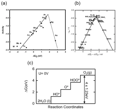
Figure 2.26. Reaction coordinates of the OER in acidic electrolyte solution. Adapted with
permission from reference112.
From the figure, one can see the Gibbs free energy of H2O and O2 species are exactly equal at an
applied bias of 1.23V (the thermodynamic potential), however the intermediate products are at different energy levels at this bias. Because the reactions happen in series, the kinetics are essentially limited by the largest energy barrier between the intermediate products. The reaction kinetic is then quantified by the current, 𝑖 according to the equation:
𝑖 = 𝑖𝑘exp (−∆𝐺𝑟
𝑘𝑇 ) Equation 2.15
Where 𝑖𝑘 is a constant, ∆𝐺𝑟 is the Gibbs free energy barrier of the rate limiting step, k is the Boltzmann constant, and T is the absolute temperature. An overpotential, or more specifically the activation overpotential, hence serves to reduce the ∆𝐺𝑟 of the rate-limiting step.
For water electro-catalysis, the best catalysts usually neither have the highest nor the lowest binding energy to the reactants, but rather have intermediate values, according to the Sabatier’s principle. As a result, when one plots the catalytic activity against the reactant binding energy,
46 one typically gets a “volcano” plot. Some of the plots for metal and binary oxide OER catalysts are shown in figure 2.27. Generally speaking, this “volvano” trend exists because too weak of binding energy leads to low conversion rate of reactants to intermediates, whereas too strong of binding energy leads to low conversion rate of intermediates to final products. The ideal catalyst is one where the energy splitting between all the intermediates are the same, as shown in figure 2.24(c) for the case of an OER catalyst. Pt and RuOx are the best metal and oxide
(non-perovskite) OER catalysts because their binding energies to the intermediates are closest to the ideal catalyst (equi-energy splitting). Note that because ORR is just the reverse of OER, one should expect the best OER catalyst to also be the best ORR catalyst.
Figure 2.27. Volcano plots. Volcano plots for (a) metallic and (b) binary oxide OER catalysts.
47
2.7 Electrodes for Solid Oxide Cells
So far we have focused on the electronic structure of catalyst which primarily affects charge transfer at the electrode/electrolyte interface. However, mass transport can also be a significant source of overpotential; in fact it often dominates in systems like solid oxide cell where gas phase diffusion and ionic transfer across the electrode/electrolyte interface are involved114,115. Fundamentally, most losses in solid oxide cell electrodes boil down to the fact that a single phase cannot conduct all three species involved in a gas phase reaction: an electron, an ion, and a gas molecule. Only an electronically conductive material can transport electrons, only an ionically conductive material can transport ions, and only a gas phase can transport a gas molecule. As a result, a complete reaction can only occur at the intersection of these three phases; this
intersection is called a triple phase boundary (TPB). Figure 2.28 shows an example of a TPB at the cathode of an oxygen-ion conducting oxide fuel cell.
Figure 2.28. Triple phase boundary. Schematic illustration of the triple phase boundary at the
cathode of an oxygen-ion conducting solid oxide fuel cell. Adapted with permission from reference114.
48 The necessity of three phases for a complete reaction not only reduces the total number of
reaction sites, it also increases the overall complexity due to added intermediate steps and species. For instance, it has been proposed that the oxygen reduction reaction happening at the cathode of a proton conducting oxide fuel cell consists of eight elementary steps, each with its own reaction order resulting in a net reaction of 𝑂2+ 4𝐻++ 4𝑒− → 2𝐻
2𝑂 (table 2.1). Because
these steps happen in series, the slowest step will be the rate-limiting step and will determine the total resistance from the electrode115. For electrodes in solid oxide cells, they are mainly
characterized by their area specific resistance (ASR), with 𝑅𝑒𝑙𝑒𝑐𝑡𝑟𝑜𝑑𝑒= 𝐴𝑆𝑅
𝐴𝑟𝑒𝑎 . Here, 𝑅𝑒𝑙𝑒𝑐𝑡𝑟𝑜𝑑𝑒 is
the total electrode resistance. ASR is not normalized to the thickness of the electrode because in most cases, the resistance of the electrode does not scale with its thickness; it is a function of extrinsic properties such as microstructure and porosity.
Table 2.1. Elementary reaction steps of ORR at the cathode of a proton conducting solid oxide fuel cell. Reproduced with permission from reference115.
In the past, to increase the area of the triple phase boundary, porous Pt was commonly used as both the anodes and cathodes. However due to the prohibitive cost of Pt and the limited added TPB from porosity alone, new methods have been employed. These methods have mainly revolved around using materials with mixed ionic and electronic conductivities (MIEC). By
49 using MIEC, one only needs the intersection of two phases for reactions to take place because one of the phases conduct both electrons and ions. As a result, the overall activity increases due to larger area where electrons, ions, and gas molecules can coexist. MIEC can exist as a one-phase material such as (La,Sr)(Co,Fe)O3-δ (LSCF) or two-phase material consisting of a
composite of electronic conductor and an ionic conductor, such as Ni-YSZ and
LSM-YSZ84,85,116,117. Schematics of operation of an MIEC cathode in a proton conducting fuel cell is shown in figure 2.29.
LSCF, a one-phase MIEC, is a perovskite oxide, where the La and Sr atoms are at the A-site, and the Co and Fe atoms are at the B-site. Sr doping induces a change in oxidation state of both the Co and Fe from +3 to +4 resulting in p-type electronic conductivity. Simultaneously, there is also charge compensation through formation of oxygen vacancies, resulting in increased oxygen-ion conductivity. As a result, LSCF has both electronic and ionic conductivities at high temperature. It is most commonly used with a ceria electrolyte. LSM ( La1-xSrxMn O3-δ ), which is typically
the electronically conductive component of a two-phase MIEC, is a perovskite where the A-site La3+ is doped with Sr with an oxidation state of +2. This acceptor doping is mainly compensated
by change in oxidation state of the Mn from +3 to +4 which results in p-type electronic conductivity. However, in this case, there is minimal change in the oxygen vacancy
concentration. LSM is usually mixed with YSZ, (oxygen ion conductor) to form a two-phase composite MIEC structure. This cathode is most commonly used on a YSZ electrolyte due to the excellent match in thermal expansion coefficients. For the anode, the most commonly used material is Ni-YSZ cermet (cermet is short for ceramic-metal), which is a two-phase composite MIEC. Ni is used due to three reasons. (1) it is one of the best HOR catalyst, (2) it is cheap, and (3) it provides mechanical support to the fuel cell, especially in cases where the electrolyte is
50 very thin. Other examples of anode include Ni-SDC (Samarium-doped ceria, SmxCe1-xO2-δ) and
Ni-GDC (Gadolinium-doped ceria, GdxCe1-xO2-δ). While the primary ionic carrier in most MIEC
is oxygen-ion, there are also MIEC such as BaCe1-xFexO3 whose main ionic conducting species
is the proton. These proton-based MIEC are typically doped BCO (BaCeO2-δ) and BZO (BaZrO 2-δ)80,115.
Figure 2.29. Active sites in different types of cathodes for a proton conducting oxide fuel cell. (a) Porous single phase electronic conductor such as Pt. (b) Two phase