HAL Id: hal-02506216
https://hal-brgm.archives-ouvertes.fr/hal-02506216
Submitted on 17 Mar 2020HAL is a multi-disciplinary open access archive for the deposit and dissemination of sci-entific research documents, whether they are pub-lished or not. The documents may come from teaching and research institutions in France or abroad, or from public or private research centers.
L’archive ouverte pluridisciplinaire HAL, est destinée au dépôt et à la diffusion de documents scientifiques de niveau recherche, publiés ou non, émanant des établissements d’enseignement et de recherche français ou étrangers, des laboratoires publics ou privés.
Controls of local geology and cross-shore/longshore
processes on embayed beach shoreline variability
Arthur Robinet, B. Castelle, Déborah Idier, M.D. Harley, K.D. Splinter
To cite this version:
Arthur Robinet, B. Castelle, Déborah Idier, M.D. Harley, K.D. Splinter. Controls of local geology and cross-shore/longshore processes on embayed beach shoreline variability. Marine Geology, Elsevier, 2020, 422, pp.106118. �10.1016/j.margeo.2020.106118�. �hal-02506216�
1
Controls of local geology and cross-shore/longshore processes on
1
embayed beach shoreline variability
2A. Robineta, B. Castelleb,c, D. Idiera, M.D. Harleyd, K.D. Splinterd
3
a BRGM, 3 Avenue Claude Guillemin, 45100 Orléans, France
4
b UMR EPOC 5805, Univ. Bordeaux, 33615 Pessac, France
5
c UMR EPOC 5805, CNRS, 33615 Pessac, France
6
d Water Research Laboratory, School of Civil and Environmental Engineering, UNSW Sydney, Manly
7
Vale, NSW, Australia
8
Corresponding author: A. Robinet, [email protected]
9
Abstract
10Shoreline variability along the 3.6-km long Narrabeen Beach embayment in SE Australia is 11
investigated over a 5-year period. We apply the one-line shoreline change model LX-Shore, 12
which couples longshore and cross-shore processes and can handle complex shoreline 13
planforms, non-erodible emerged headlands and submerged rocky features. The model 14
skilfully reproduces the three dominant modes of shoreline variability, which are by 15
decreasing order of variance: cross-shore migration, rotation, and a third mode possibly 16
related to breathing. Model results confirm previous observations that longshore processes 17
primarily contribute to the rotation and third modes on the timescales of months to seasons, 18
while cross-shore processes control the shoreline migration on shorter timescales from hours 19
(storms) to months. Additional simulations simplifying progressively the bathymetry show 20
how the inherent geology strongly modulates the spatial modes of shoreline variability. The 21
offshore central rocky outcrop is found to limit the rotation. In contrast, the submerged rocky 22
platforms that extend from the headlands enhance the shoreline rotation mode and increase 23
alongshore variability of the cross-shore migration mode, owing to increased alongshore 24
variability in wave exposure. Offshore wave transformation across large-scale submerged 25
rocky features and headland shape are therefore critical to contemporary shoreline dynamics. 26
2
Keywords
27
Embayed beach; shoreline model; local geology; rotation; cross-shore migration; wave 28
transformation 29
1
Introduction
30
In the context of climate change and increased anthropogenic pressures, it is critical to improve 31
our understanding and predictive capacity of the spatiotemporal evolution of the land-sea 32
interface. Modelling this shoreline variability is challenging given the myriad of driving 33
processes acting at different timescales. Along wave-dominated open and uninterrupted 34
sandy coasts, shoreline variability on the timescales from hours (storm) to years is often 35
primarily driven by cross-shore processes with the shoreline moving rapidly landward 36
(erosion) during storms, and slowly seaward (accretion) during calm periods (e.g. Yates et al., 37
2009). On longer timescales, other processes such as changes in sediment supply (Thom, 1983) 38
and sea level rise (e.g. Bruun, 1962; Le Cozannet et al., 2016) become important, as well as 39
longshore processes. However, the typical timescales associated with these processes mostly 40
differ on embayed beaches, where inherent geology (rocky headlands, submerged outcrops 41
and rocky platforms extending from the headlands) greatly complicates shoreline response, 42
with longshore processes also impacting shoreline response on short timescales (Ojeda and 43
Guillen, 2008). 44
Embayed sandy beaches are ubiquitous along hilly or mountainous wave-exposed coasts 45
(Short and Masselink, 1999). The geometry of embayed beaches (headland and beach length) 46
depends on the inherent geology (Fellows et al., 2019), which together with exposure to 47
prevailing wave climate dictate beach morphodynamics (Castelle and Coco, 2012; Daly et al., 48
3 2014) and shoreline change (e.g. Turki et al., 2013). A well-known shoreline behaviour along 49
embayed beaches is clockwise/counterclockwise beach rotation (Klein et al., 2002; Short and 50
Trembanis, 2004; Ranasinghe et al., 2004; Ojeda and Guillen, 2008; Thomas et al., 2010; Loureiro 51
et al., 2013; Turki et al., 2013; Van de Lageweg et al., 2013). While rotation has been observed 52
on the scale of individual storm events (e.g. Harley et al., 2013) and more gradually due to 53
seasonal changes in wave conditions (e.g. Masselink and Pattiaratchi, 2001), it has historically 54
been attributed to longshore sediment transport with the dominant direction of sand 55
movement being associated with the dominant incident wave direction. More recently, Harley 56
et al. (2015) suggested a more complex rotation process whereby alongshore variability in 57
cross-shore sediment fluxes may be more significant at Narrabeen-Collaroy embayment (SE 58
Australia). In addition, other modes of shoreline variability can be observed, such as a so-59
called ‘breathing’ mode that represents a change in the overall curvature of the embayed beach 60
(Ratliff and Murray, 2014; Blossier et al., 2017). This mode has been shown theoretically to be 61
driven by longshore processes and to typically explain much less variability of shoreline 62
change than the rotation mode (Ratliff and Murray, 2014). 63
Over the last decade, a wealth of numerical models has been developed to simulate and further 64
understand shoreline change within coastal embayments. Most of these models are one-line 65
models where shoreline change is essentially driven by longshore processes (e.g. Turki et al., 66
2013; Ratliff and Murray, 2014). More recently, shoreline change models coupling cross-shore 67
and longshore processes have emerged (Vitousek et al., 2017; Robinet et al., 2018; Antolínez et 68
al., 2019). Amongst these models, LX-Shore (Robinet et al., 2018) can handle complex shoreline 69
geometries (e.g. sand spits, islands), including non-erodible areas such as coastal defences and 70
headlands. New developments to the model also account for non-erodible submerged rocky 71
4 structures, providing a unique tool to address the control of geology and cross-shore and 72
longshore processes on shoreline changes in coastal embayments. Although it is well 73
established that both cross-shore and longshore processes combine together to drive shoreline 74
variability along embayed beaches, to our knowledge there is no shoreline modelling study 75
coupling cross-shore and longshore processes and addressing embayed beach dynamics. In 76
addition, most of the modelling studies assume idealized embayed beach bathymetries (e.g. 77
Turki et al., 2013; Ratliff and Murray, 2014). However, it is anticipated that offshore wave 78
transformation over complex bathymetries can have a strong impact on alongshore breaking 79
wave characteristics and, in turn, sediment transport and shoreline response. 80
The objectives of the present study are two-fold: (1) to identify the respective contributions of 81
cross-shore and longshore processes to the different modes of shoreline variability at a real 82
embayed beach; and (2) to investigate the role of the inherent geology in modulating the spatial 83
and temporal modes of shoreline change. This work relies on the combination of a unique, 84
high-resolution dataset collected at the embayed beach of Narrabeen-Collaroy, SE Australia, 85
and the further application of the LX-Shore one-line shoreline change model. The study site 86
and the LX-Shore model physics are described in detail in Sections 2 and 3, respectively. Model 87
results are then analysed both in terms of spatial and temporal variability in Section 4. Results 88
are discussed in Section 5 before conclusions are drawn in Section 6. 89
2
Study site
90The Narrabeen-Collaroy embayment is a 3.6 km long sandy beach (Turner et al. 2016) located 91
in the northern coastal area of Sydney, Australia (Fig 1a,c), which is hereafter referred to as 92
Narrabeen for conciseness. The sediment is nearly uniform along the embayment and consists 93
of fine to medium quartz sand with a median grain size (d50) of approximately 300 µm (Turner 94
5 et al. 2016). The beach is bordered by two rocky headlands, which extend offshore through 95
large submerged rocky platforms, with the southern headland being the most prominent (Fig 96
1c). Just south of the northern headland, an intermittently-active inlet (typically 50 m wide) 97
occasionally connects an inland lagoon to the ocean, which acts more as a sink than a source 98
of sediment to the beach (Morris and Turner, 2010). 99
The tide at Narrabeen is microtidal and semidiurnal with a mean spring tidal range of 1.3 m 100
(Turner et al. 2016). The beach is exposed to moderate- to high-energy wave conditions with a 101
mean significant wave height (Hs) of 1.6 m and a mean peak period (Tp) of 10 s. The wave 102
climate is dominated by long period swells coming from the SSE (Fig 1.b), generated by 103
eastward-tracking extratropical cyclones south of mainland Australia. The coast is also 104
exposed to storm waves from the S, E and NE generated by intensified extratropical cyclones, 105
east coast lows, and tropical cyclones, respectively. The wave climate is slightly seasonally-106
modulated owing to decreasing extratropical cyclone and east coast low activity in the austral 107
summer along with more NE sea breezes generating short-period waves. The wave climate 108
offshore of Narrabeen is termed storm-dominated as energetic wave conditions occur all year 109
long (Splinter et al., 2014). 110
Nearshore wave conditions at Narrabeen are non-uniform alongshore due to refraction, 111
bottom friction and depth-induced breaking enforced by the complex inherent geology (Fig. 112
1c). The south headland shelters the southern part of the beach from waves coming from the 113
S-SE (Bracs et al., 2016), leading to up to 30% difference in breaking wave height from S to N 114
for average conditions (Harley et al., 2011a). Within the embayment, the bottom is essentially 115
sandy from the subaerial beach to at least 20-m depth. Exceptions to this sandy bed are made 116
in front of the northern and southern end of the beach, where small rocky outcrops lying in 117
6 depths from 5 to 10 m disturb the relatively shore-parallel bathymetric iso-contours. Apart 118
from relatively small rocky areas, a large rocky outcrop is observed approximately 1 km 119
offshore in the centre of the embayment, with a minimum depth at its crest of approximately 120
18 m (Fig 1b). Previous wave modelling suggests that, during energetic storm events, this 121
geological feature affects wave propagation through a combination of refraction, diffraction 122
and bottom friction (Bracs et al., 2016). 123
The beach state is modally intermediate-dissipative in the north and progressively transforms 124
into intermediate-reflective towards the S. The subaerial beach width can vary by up to 80 m 125
(70 m) in the north (south). The beach is backed by high natural and vegetated foredunes in 126
the north, while in the central and southern part of the beach intensive urbanization has led to 127
the replacement of natural dunes by sea-facing properties typically protected by buried rubble 128
mound sea-walls. 129
A continuous beach survey program has been led since 1976 at Narrabeen, creating one of the 130
most extensive shoreline datasets worldwide (Turner et al., 2016). Among the numerous cross-131
shore transects initially defined to support this program, five (PF1, PF2, PF4, PF4 and PF8) 132
have been continuously used to conduct biweekly beach profiles (transects are shown in Fig. 133
1b). Since 2005, this survey program has included monthly three-dimensional topographic 134
surveys of the entire 3.6 km-long subaerial beach using an all-terrain vehicle (Harley et al., 135
2011b). Previously, Harley et al. (2015) performed an empirical orthogonal function (EOF) 136
analysis on a 5-year period (2005-2010) of this three-dimensional dataset and showed that the 137
two dominant modes of shoreline variability are cross-shore migration followed by rotation, 138
explaining approximately 55% and 22% of the overall variability, respectively. A third mode 139
of variability explaining less than 10% of the total variance was disregarded in their analysis. 140
7 Below we address the same period as that investigated in Harley et al. (2015), but focussing on 141
shoreline variability from both measurements and model outputs. 142
3
LX-Shore application
143
3.1 Model description 144
LX-Shore is a two-dimensional planview cellular-based one-line shoreline change model for 145
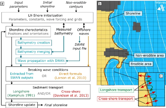
wave dominated sandy coasts (Robinet et al., 2018). An overview of the model is provided in 146
Fig. 2 and the reader is referred to Robinet et al. (2018) for more details. LX-Shore simulates 147
shoreline change resulting from the combination of gradients in total longshore sediment 148
transport and cross-shore transport driven by changes in incident wave energy (Fig 2a,c). LX-149
Shore can handle complex shoreline geometries (e.g. sand spits, islands), including non-150
erodible areas such as coastal defences and headlands. 151
Unlike usual one-line models directly resolving the shoreline position (e.g. Hanson, 1989; 152
Kaergaard and Fredsoe, 2013; Hurst et al., 2015; Vitousek et al., 2017), and in line with Ashton 153
and Murray (2006), LX-Shore computes changes in the relative amount of dry (i.e. land) surface 154
in square cells discretizing horizontally the computation domain and presenting a typical 155
spatial resolution of 10-100 m (Fig. 2b). This relative amount, hereafter referred to as the 156
sediment fraction, ranges from 0 (water cells) to 1 (fully dry cells). The planview shoreline is 157
then retrieved at each simulation timestep using an interface reconstruction method. Change 158
in sediment fraction within the cells can result from longshore transport computed using the 159
formula of Kamphuis et al. (1991), which can be multiplied by a free calibration parameter (fQl)
160
when data is available for calibration. Sediment fraction changes also result from cross-shore 161
transport using an adaptation of the equilibrium-based ShoreFor model (Davidson et al., 2013; 162
8 Splinter et al., 2014). Here the disequilibrium term is computed from offshore wave conditions 163
instead of breaking wave conditions. This cross-shore module is based on three model free 164
calibration parameters (for more detail the reader is referred to Davidson et al., 2013; Splinter 165
et al., 2014): the response factor Φ that describes the ‘memory’ of the beach to antecedent wave 166
conditions; the rate parameter c that describes the speed at which the shoreline 167
erodes/recovers; and a linear trend parameter b. 168
LX-Shore incorporates the direct formula of Larson et al. (2010) to rapidly compute the wave 169
characteristics at breaking at each time step, which is typically used on simple and academic 170
application cases (Robinet et al., 2018). Here the coupling with the spectral wave model SWAN 171
(Booij et al., 1999) is used to account for the complex wave transformation at Narrabeen. LX-172
Shore, in turn, provides at each time step an updated bathymetry that feeds back onto wave 173
transformation. This updated bathymetry is reconstructed (Fig. 2a) using a method similar to 174
the one used by Kaergaard and Fredsoe (2013), from the current shoreline position and an 175
idealized static equilibrium beach profile (a Dean profile). 176
For the present study, the bathymetric reconstruction method presented in Robinet et al. (2018) 177
has been improved by allowing real non-erodible bathymetric features to be included in water 178
depths greater than a threshold depth (Dt). Beyond this depth, the idealized bathymetry is 179
replaced by the measured bathymetry. Dt must be greater than the depth of closure (Dc) to 180
maintain the equilibrium beach profile which is a fundamental assumption of the one-line 181
modelling approach. Note that a merging is applied over a buffer area between Dc and Dt to 182
ensure a smooth transition between idealized and measured bathymetries. This improvement 183
allows testing the effect of complex local geology such as that observed at Narrabeen on the 184
different modes of shoreline variability. 185
9 3.2 Data
186
3.2.1 Waves and wind 187
LX-Shore simulations are conducted using offshore wave conditions (Hs, Tp and peak wave 188
direction Dp) measured by the Sydney buoy located 11 km to the southeast of Narrabeen in 189
approximately 80-m depth. Similar to Harley et al. (2015), gaps in buoy measurements were 190
filled using wave conditions extracted from the CAWCR hindcast (Durrant et al., 2014). 191
Inshore wave conditions measured by a waverider buoy deployed at the centre of the 192
embayment in 10-m depth from July 21 to November 14, 2011 were also used to validate the 193
modelled wave conditions close to breaking. As justified in section 3.4, SWAN was also forced 194
by the wind conditions measured at Sydney airport. 195
3.2.2 Bathymetry and seabed type 196
Three different bathymetric data sources were used to generate the bathymetries associated 197
with the SWAN computation grids introduced in Section 3.3.3. The first, most-inshore, 198
bathymetry was sourced from sixteen surveys conducted using a single-beam echosounder 199
mounted to a jetski within the Narrabeen embayment between April 2011 and May 2017. These 200
sixteen bathymetries were averaged to obtain a representative bathymetry of the embayment. 201
Remaining gaps in the bathymetry over the LX-Shore simulation domain were subsequently 202
filled using a second bathymetric dataset of 2-m-spaced iso-bathymetric contours covering the 203
Sydney coastal waters down to 50 m depth digitised from bathymetric charts by the NSW 204
Office of Environment and Heritage (NSW OEH). For even deeper waters, the large-scale 205
coarse-resolution Australian Bathymetry and Topographic Grid (ABTG, Whiteway, 2009) was 206
used. Rocky seabed contours were extracted from the mapping of subtidal habitats provided 207
10 by the NSW OEH and used to identify the non-erodible rocky patches within and outside the 208
embayment. 209
3.2.3 Shoreline and rocky contours 210
Contours of the northern and southern Narrabeen headlands were digitalized manually from 211
Google Earth. For LX-Shore calibration and validation, 44 complete planview shorelines 212
derived from the all-terrain vehicle topographic surveys conducted from July 2006 to July 2010 213
with an average periodicity of 30 days were used (Harley et al., 2015). Following Harley et al. 214
(2015), the mean-sea-level contour was used as the shoreline proxy throughout. The beach 215
topographic survey conducted on July 22, 2005 was also used to compute the initial shoreline 216
position in our simulations as detailed in Sections 3.3.1 and 3.3.2. 217
3.3 Setup 218
3.3.1 General settings 219
The model is applied over a 5-year period from July 2005 to July 2010, which is the period 220
studied in the reference work of Harley et al. (2015). The simulation timestep is set to 3 hours 221
for both LX-Shore and SWAN. The equilibrium beach profile used in LX-Shore was calibrated 222
using the time and spatial average of the beach profiles measured along transects PF2, PF4 and 223
PF6 (Fig. 1b) down to nearly 14-m depth. PF1 and PF8 were excluded due to the prominence 224
of rocky outcrops at these locations. The depth of closure used in LX-Shore simulations was 225
obtained from the following steps: (i) offshore wave conditions from July 2005 to July 2010 226
were propagated shoreward using SWAN, based on the computation grids and model settings 227
described in Sections 3.3.3 and 3.4, respectively; (ii) wave conditions were extracted in 10-m 228
depth offshore the five historical transects and then used to estimate a few theoretical values 229
of Dc along the beach, based on the formula of Hallermeier (1981); (iii) because estimates of Dc 230
11 ranged from 6.2 to 8 m, a near average value of 7 m was taken as representative of Dc for the 231
entire embayment. The implications related to the choice of this depth of closure are discussed 232
later in Section 5.2. 233
3.3.2 Initial conditions 234
The rocky contours are considered non-erodible and remain unchanged during the model 235
simulations. The initial shoreline condition is the planview shoreline measured by the all-236
terrain vehicle on July 22, 2005. However, preliminary tests showed that the mean shoreline 237
planform simulated with LX-Shore tends to slowly converge towards a slightly different shape 238
than that observed, which is a common problem in shoreline change modelling (e.g. Antolínez 239
et al., 2019). Given that the objective of the present study is to investigate the spatial and 240
temporal shoreline variability and not the mean shoreline planform, the deviation from the 241
respective mean of the modelled and measured shoreline was compared. To avoid bias 242
induced by model spin-up from the initial measured shoreline position, a two-step simulation 243
workflow was designed (see Fig. 3). First, a spin-up simulation was run from the initial 244
measured shoreline position to obtain a quasi-converged planview shoreline by averaging the 245
planview shoreline simulated during the last year of the simulation period. Then, this quasi-246
converged planview shoreline was used as input to a new simulation over the same period. 247
Because the first year of this second simulation still involves some model spin-up, it is 248
removed from further analyses, therefore the results presented here concentrate only on the 4-249
year period from July 2006 to July 2010. 250
3.3.3 Computation grids and role of inherent geology 251
A modelling strategy using a nested SWAN computation grid was adopted to speed up the 252
simulations (Fig. 4a). The coarser hydrodynamic grid is regular with a mesh resolution of 50 m 253
12 and is based on a bathymetry computed by merging the 2 m iso-contour bathymetry with the 254
deeper ABTG bathymetry (Fig. 4a). Depths from the 2 m iso-contour dataset are kept from 0 255
to nearly 40 m depth and are then progressively merged with the coarser ABTG bathymetry 256
data down to nearly 50 m depth, below which only ABTG data are used. 257
The nested refined hydrodynamic grid is regular, with a 20-m mesh, and is based on the 258
bathymetry produced iteratively by LX-Shore as described in Section 3.1. The measured 259
bathymetry used in the merging process is made of the combination of the time-averaged 260
jetski-based bathymetries and the 2 m iso-contour dataset. Fig. 4b shows an example of the 261
merged bathymetry produced by LX-Shore. The morphological grid used in LX-Shore (Fig. 4c) 262
has the same spatial extent as the refined hydrodynamic grid but with a cell width of 80 m. 263
The shoreline is discretized into nearly 40 cells. To explicitly test the influence of the inherent 264
local geology on the different modes of shoreline variability at this embayed beach, additional 265
simulations were performed using alternative bathymetries for the refined grid. The central 266
rocky outcrop was removed from the nearshore bathymetry (Fig. 5b) and the bathymetry was 267
also further idealized by removing submerged rocky platform headland extensions and 268
replacing it with a Dean profile along the entire embayment (Fig. 5c), showing large seabed 269
elevation differences (Fig. 5d). 270
3.4 Calibration 271
Prior to LX-Shore simulations, a preliminary task consisted of calibrating SWAN parameters 272
to improve wave hindcasts within the embayment. Calibration was made using inshore wave 273
conditions measured at the centre of the embayment in 10-m depth (Fig. 4a,b white triangle) 274
from July 21 to November 14, 2011 (no other observations were available during the simulation 275
period). The default directional spreading of 30° was increased to 45°. The friction was enabled 276
13 using the expression of Madsen et al. (1988) and a non-uniform bottom roughness length scale. 277
The default value of 0.05 m was used for sandy seabed, but this value was set to 0.5 m for 278
rocky seabed. Finally, the wave generation by wind and dissipation through whitecapping 279
were enabled using the expressions of Komen et al. (1984). Modelled Hs and mean wave 280
direction (Dm) show good skill (Table 1) with a root mean squared error (RMSE) of 0.17 m and 281
10.13° and with a correlation coefficient of 0.94 and 0.75, respectively. Modelled mean wave 282
period (Tm) is less accurate with a RMSE of 1.54 s and a correlation coefficient of 0.60. The 283
present, more-refined, model setup reduces the bias in Dm from 4° to 0.71° in comparison with 284
the reference look-up table used to predict inshore waves at Narrabeen in Turner et al. (2016). 285
The cross-shore model was calibrated by optimizing three free model parameters. Here, a 286
simulated annealing optimization algorithm (Bertsimas et al., 1993) was used as in Castelle et 287
al. (2014) to find the optimal coefficient combination to simulate the cross-shore shoreline 288
positions measured at PF6. The optimized values for these coefficients are as follows: Φ = 35 289
days; c = 2.5304 x 10⁻⁷ m1.5s-1W-0.5; b = 1.4695 x 10⁻⁷ ms-1 and were further used for the entire
290
embayment. For the longshore transport model, simulations were conducted by increasing fQl
291
to 3, 4 and 5. A fair comparison regarding the changes of the overall shoreline orientation 292
(defined as the angle between the north and the linear fit of the northward shoreline positions) 293
was achieved for fQl = 4.
294
3.5 Post-processing of shoreline position 295
To ease the analysis of measured and simulated shoreline change, the Cartesian coordinates 296
(x,y) of shoreline positions were transformed into alongshore – cross-shore (s,p) coordinates 297
following the method introduced by Harley and Turner (2008). This transformation relies on 298
a logarithmic spiral baseline obtained by fitting a reference planview shoreline. Here, the 299
14 average planview shoreline over the study period without model spin-up (July 2006 – July 300
2010) is used as the reference, with p indicating the cross-shore distance from the time-301
averaged cross-shore shoreline position and s indicating the alongshore distance from the 302
northern end of the beach. Because of the slight differences between the measured and 303
modelled time-averaged shoreline planforms, two distinct logarithmic spirals were used as 304
reference planforms to analyse shoreline variability (one for the model, one for the 305
observations). These two distinct reference planforms were used to more accurately define the 306
longshore and cross-shore directions in the measured and modelled datasets. 307
4
Results
308
4.1 Simulated shoreline changes 309
Fig. 6a shows the observed and simulated time-averaged planview shorelines. Although the 310
overall shape is fairly well captured by the LX-Shore model, substantial changes of up to 30-311
40 m cross-shore can be observed (Fig. 6b). The planform curvature is underestimated by the 312
model, resulting in a mean modelled shoreline position located further offshore in the centre 313
of the embayment and further inshore close to its extremities. Although accurately simulating 314
the mean shoreline planform of the coastal embayment is not an objective of the present study, 315
this limitation will be discussed later in the paper (refer Section 5). Hereafter, the cross-shore 316
deviation of observed and modelled shoreline from their respective means p(s,t) is addressed. 317
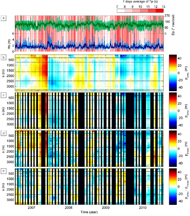
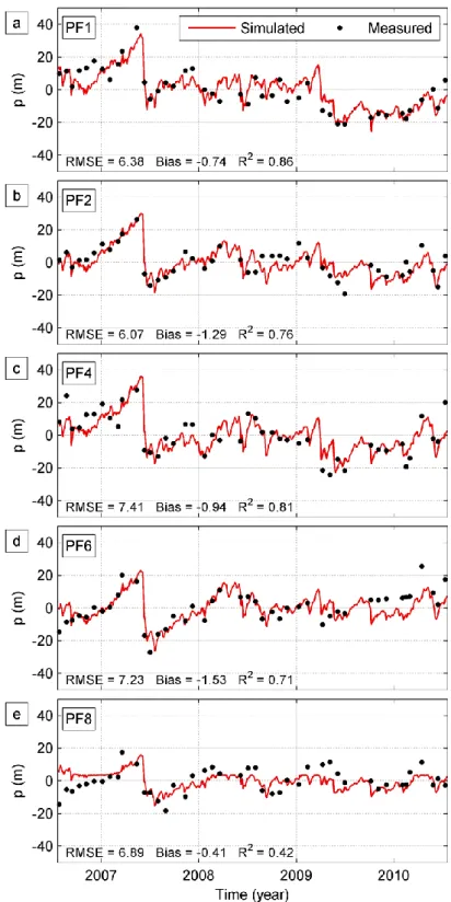
Fig. 7 shows the space-time diagrams of the modelled (Fig. 7b,c) and measured (Fig. 7d) 318
shoreline deviation from the mean with corresponding time series of the five historical profiles 319
(PF1, PF2, PF4, PF6 and PF8) shown in Fig. 8. A number of erosion events along the entire 320
embayment can be seen. The June 2007 event stands out (Fig. 7b-d), which was caused by an 321
15 intense east coast low in the northern Tasman Sea on 7-10 June driving high-energy waves 322
from the SE reaching 6.9 m offshore (Fig. 7a), and resulting in 273,000 m3 of sand removed
323
from the subaerial beach (Harley et al., 2015). The shoreline retreat due to this event was 324
observed to be on the order of 30-40 m at all five profiles, except at the southern profile PF8 325
where erosion reduced to approximately 20 m (Fig. 8). Rapid erosion events were followed by 326
slower recovery periods typically extending a few months (Fig. 7d). Overall, shoreline varied 327
more at the north of the embayment than at the south, owing to the larger exposure to the 328
prevailing wave conditions from the SE (Harley et al., 2015). A number of clockwise and 329
counter-clockwise rotation events can be observed (Fig. 7d), which are sometimes not 330
associated with an overall migration of the shoreline. 331
Similar shoreline change patterns are observed with the model (Fig. 7c), which can provide 332
much higher frequency insight into erosion and rotation signals using output at each model 333
time step (Fig. 7b). The model readily captures erosion and subsequent multi-month recovery 334
of the shoreline, as well as rotation events (Fig. 7c-e). Given that the model does not explicitly 335
include surfzone sandbar dynamics, the model does not capture the short-scale, alongshore 336
shoreline variability (e.g. around May 2009), which may reflect the presence of megacusp 337
embayments observed previously at this site (e.g. Harley et al., 2015; Splinter et al., 2018). Fig. 338
7b also shows that shoreline recovery is not a steady process, instead, significant interruptions 339
and reversals in recovery are caused by more or less small storm events. This is further 340
emphasized in Fig. 8. The model systematically explains more than 70% of shoreline variance 341
at all transects (Fig. 8) except at the southern profile FP8 (42%, Fig. 8e), with root mean squared 342
errors systematically smaller than 7.5 m (Fig. 8). Importantly, the model is also able to capture 343
16 extreme accretion-erosion events, which were typically underestimated north of the beach in 344
previous modelling efforts (e.g. Splinter et al., 2014). 345
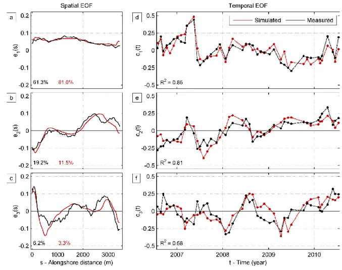
4.2 Temporal and spatial modes of shoreline variability: LX-Shore capabilities 346
To better understand the different modes of shoreline variability within the embayment, an 347
EOF analysis was performed to decompose observed shoreline variability into linear 348
combinations of statistically independent spatial and temporal patterns (Miller and Dean, 349
2007). Results of the first three EOFs from measured cross-shore shoreline deviation from the 350
mean p(s,t) (Fig. 7d) are presented in Fig. 9. These results indicate very similar modes of 351
shoreline variability to those obtained in Harley et al. (2015). This is in spite of the fact that the 352
former study includes an additional one year of shoreline data that is disregarded here due to 353
model spin-up. The primary modes of shoreline variability are, by decreasing order of 354
importance: (i) cross-shore migration with larger amplitude in the north and accounting for 355
61.3% of the variance; (ii) beach rotation accounting for 19.2% of the variance and presenting 356
a nodal point near s = 1800 m and an attenuation of the spatial mode at s = 800 m; (iii) a third 357
mode accounting for 6.2% of the variance. 358
A similar analysis was performed with model outputs at time steps concurrent with 359
measurements (Fig. 7c). Results (Fig. 9, red lines/dots) show that the EOF analysis gives, in the 360
same order of importance, very similar spatial patterns (Fig. 9a-c), although the model gives 361
more variance (81.6%) to the first mode (cross-shore migration) than measurements (61.3%). It 362
is however important to note that the model was not calibrated on these modes of variability, 363
and that slight changes in the free parameters could lead to better agreement, which will be 364
discussed later in the paper (refer Section 5). The corresponding modelled temporal modes of 365
17 variability are also in very good agreement with measurements, particularly for the two first 366
modes (R2 > 0.8) and to a lesser extent the third one (R2 = 0.68, Fig. 9d-f).
367
4.3 Respective contribution of longshore and cross-shore processes to shoreline 368
variability on the timescales from storm to years 369
Because modelled temporal and spatial modes of shoreline variability are in very good 370
agreement with observations, LX-Shore can be used to further address the respective 371
contributions of cross-shore and longshore processes to the different modes of shoreline 372
variability. For this purpose, cross-shore or longshore processes were switched off 373
alternatively and the impacts on the modes of shoreline variability were investigated 374
systematically. Using model outputs at each model time step (3 hours) instead of only at the 375
time steps concurrent with measurements (~monthly), also provides insight into the shoreline 376
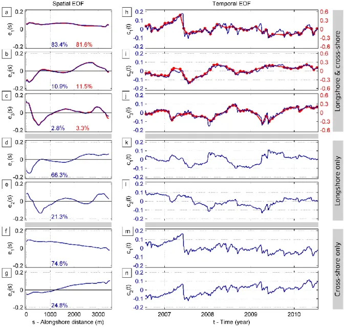
response timescales. The three top panels in Fig. 10 show the first three EOFs with both cross-377
shore and longshore processes included. Spatial modes (cross-shore migration, rotation and 378
the third mode) are essentially similar in pattern (Fig. 9a,b,c), with the high-frequency 379
temporal modes showing a large number of reversals and short-term large changes 380
highlighting the dynamic nature of the embayment. Visual inspection of Fig. 10h,i,j 381
(comparison of blue lines) also reveals different temporal dynamics for the three modes of 382
variability. While the cross-shore migration mode occurs on scales of hours (storm) to months 383
(Fig. 10h), the rotation mode operates more gradually on annual and interannual scales (Fig. 384
10i). This is in line with Harley et al. (2015) who showed that the first EOF was controlled by 385
waves averaged over ~ 8 days (representing storms) whereas the second EOF was more 386
controlled by wave changes over months to seasons. Regarding the third mode, no 387
18 predominant timescale arises as both short-term (event scale) and long-term (annual scale) 388
temporal patterns superimpose. 389
Running LX-Shore with cross-shore processes switched off (i.e. longshore only), the EOF 390
analysis shows that the primary modes of shoreline variability in such a configuration (Fig. 391
10d,e) are essentially similar in pattern to the second (rotation) and third modes (Fig. 10b,c). 392
The corresponding temporal modes (Fig. 10k,l) are also essentially the same as for the 393
simulation combining cross-shore and longshore processes (Fig. 10i,j). Running LX-Shore with 394
longshore processes switched off (i.e. cross-shore only), the EOF decomposition leads to two 395
dominant modes of shoreline variability (Fig. 10f,g,m,n). The first mode corresponds to a 396
short-term cross-shore shoreline migration, which is maximized along the northern part of the 397
beach and decreases to close to 0 towards the south (Fig. 10f,m). The negative trend in the 398
temporal EOF, combined with the shape of the spatial EOF, indicates that during the 399
simulation this first mode tends to drive a long-term shoreline retreat, which increases 400
northwards. In contrast, the second mode corresponds to a beach rotation with an amplitude 401
maximized along the southern part of the beach (Fig. 10g,n). The positive trend in the temporal 402
EOF, combined with the shape of the spatial EOF, indicates that during the simulation this 403
second mode tends to drive a long-term shoreline retreat and advance at north and south, 404
respectively. Given that the temporal EOFs of these two modes are similar, and that the first 405
mode shows more variance, the combination of these two modes mostly corresponds to the 406
cross-shore migration mode of the LX-Shore simulation accounting for both cross-shore and 407
longshore processes. In brief, LX-Shore simulations indicate that longshore processes 408
primarily contribute to the second (rotation) and third modes of shoreline variability (Fig. 409
10b,c), while cross-shore processes control the cross-shore migration with more variability at 410
19 the northern end (Fig. 10a). These results corroborate those of Harley et al. (2011a, 2015) based 411
on extensive field data analysis, showing that LX-Shore can be a powerful tool to address the 412
modes of shoreline variability in complex settings. 413
4.4 Controls of inherent local geology on the shoreline modes of variability 414
As shown in Fig. 1b, Narrabeen is bordered by two prominent and morphologically different 415
rocky headlands, which extend offshore through large submerged rocky platforms. In 416
addition, a large rocky outcrop located approximately 1.5 km offshore in less than 20-m depth 417
can be observed. This inherent local geology can affect wave propagation, breaking wave 418
conditions along the embayment and, in turn, the modes of shoreline variability. To further 419
test this hypothesis, two additional simulations (including wave and shoreline modelling) 420
were performed using the same free parameters as in the reference simulation: one removing 421
the prominent central rocky outcrop (Fig. 5b) and a second simulation further removing the 422
headland-facing submerged rocky platforms (including the central rocky outcrop) through a 423
Dean profile along the entire embayment (Fig. 5c). 424
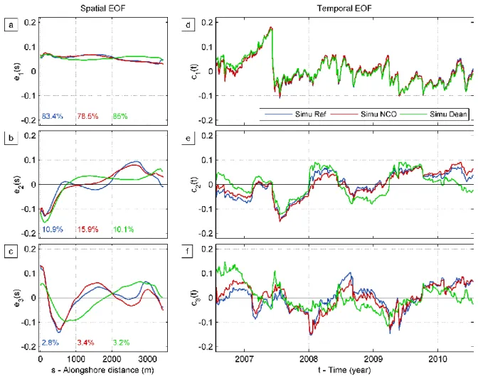
Results from EOF decomposition applied to the outputs of these two additional simulations 425
are superimposed in Fig. 11 onto those from the reference simulation. It appears that removing 426
the central rocky outcrop only slightly affects the overall modes of shoreline variability (Fig. 427
11, red lines). This suggests that the outcrop is too deep to enforce strong wave energy focusing 428
that would cause alongshore gradients in breaking wave conditions large enough to modify 429
both modal wave exposure and longshore sediment transport patterns. This is illustrated in 430
Fig. 12 that shows that even for representative prevailing high-energy waves from the SSE, the 431
wave height patterns alongshore (Fig. 12b) are very similar to those simulated with the 432
reference bathymetry (Fig. 12b,d,e). Two substantial effects can however be highlighted. First, 433
20 the spatial pattern of the second (rotation) mode is more uniform alongshore (Fig. 11b), 434
suggesting that the presence of this relatively deep central rocky outcrop increases shoreline 435
response complexity. Second, the importance of the rotation mode increases by approximately 436
46% (from 10.9% to 15.9% of the total variance, Fig. 11b) when removing the outcrop, 437
suggesting that the central rocky outcrop is a limiting factor to the rotation signal of the 438
embayment. The simulation for which the bathymetry is further idealized (i.e., with the 439
submerged rocky platforms at the two extremities also removed, refer Fig. 5c) shows much 440
larger changes on shoreline variability (Fig. 11, green lines). The first (cross-shore migration) 441
mode is more uniform along the embayment (Fig. 11a). This observation is consistent with 442
Harley et al. (2015), who suggest that the asymmetric spatial EOF of the cross-shore migration 443
mode is related to alongshore variability in wave exposure, which is indeed reduced when 444
idealizing the offshore bathymetry (see wave field for a SSE swell in Fig. 12c). Overall, the 445
spatial patterns of the second (rotation) and third modes are also more uniform along the 446
embayment without the complex submerged rocky platforms. In addition, the contribution of 447
the second (rotation) mode is reduced by 36% with respect to simulations where only the 448
central rocky outcrop is removed (from 15.9% to 10.1%). This suggests that the prominent 449
submerged rocky platform extensions from the headlands enhances the shoreline rotation 450
mode at Narrabeen. Wave refraction around the prominent platforms resulting in more 451
alongshore non-uniform breaking wave conditions and, in turn, stronger longshore sediment 452
transport gradients, is therefore hypothesized to increase the degree of shoreline rotation. 453
21
5
Discussion
454
5.1 Respective contributions of inherent geology and cross-shore and longshore 455
processes 456
For the first time our simulations allowed isolating the respective influence of the inherent 457
geology and the cross-shore and longshore processes on the dominant spatial and temporal 458
modes of shoreline variability at a real embayed beach. Although our findings cannot be 459
generalized to all coastal embayments, they provide new insight into shoreline dynamics on 460
real embayed beaches. Overall our results show that longshore processes primarily contribute 461
to the second (rotation) and third modes of shoreline variability at this site, while cross-shore 462
processes control the alongshore-averaged, cross-shore migration, with the inherent geology 463
modulating the modes in space. An important result is that the inherent geology can have a 464
significant impact on shoreline dynamics from the timescales of storms to years. Inherent 465
geology has long been known to influence beach states (Jackson et al., 2005), rip channel 466
morphodynamics (Castelle and Coco, 2012; Daly et al., 2014) or extreme erosion (Loureiro et 467
al., 2012). Here we demonstrate that not only does the headland geometry have an impact on 468
shoreline change, but also more localised submerged rocky outcrops both at the centre and 469
extremities of the embayment. The influence of such submerged non-erodible morphology has 470
been disregarded in previous shoreline change studies, except in a few studies such as Limber 471
et al. (2017) who only investigated the time-averaged shoreline position. These results have 472
implications from the perspective of coastal engineering. Hard structures such as groynes 473
(Hanson et al., 2002) or submerged breakwaters (Bouvier et al., 2017, 2019) are often designed 474
based on their impacts on the adjacent mean shoreline position. Here we show that the design 475
of such structures should also consider their impact on the modes of shoreline variability, 476
22 including beach rotation and other higher-order modes. These can indeed drive localized time-477
limited severe erosion on artificial embayed beaches (Ojeda and Guillen, 2008). 478
The third mode of shoreline variability, which is reasonably reproduced by the model (Fig. 479
9c), was suggested by Harley et al. (2015) to potentially be driven by ebb inlet processes 480
occurring at the northern extremity of the beach. The inlet, however, is not included in LX-481
Shore, which suggests that the influence of the inlet on the shoreline variability is relatively 482
minor and that this third mode is related to other processes. An alternative control of this third 483
mode of shoreline variability is the localized rocky outcrop located in 5 to 10 m depths towards 484
the northern extremity of the beach at around s = 150 m. Indeed, when present in the 485
bathymetry, this rocky outcrop is observed to cause substantial localized focusing of breaker 486
wave energy (Fig. 12a,b,d, s = 150 m). With this rocky outcrop smoothed within an idealized 487
bathymetry, relatively uniform longshore breaker wave heights are observed (Fig. 12c,d, s = 488
150 m), resulting in weakly spatially varying longshore transport. In contrast, such inherent 489
geology, which results in stronger alongshore variability in breaking wave characteristics and, 490
in turn, longshore transport, is likely to drive more complex shoreline variability in its lee. The 491
shape of the spatial EOF of the third mode becomes more symmetrical when idealizing the 492
bathymetry (Fig. 11c) and resembles the U-shaped breathing pattern identified in Ratliff and 493
Murray (2014). The translation of the U-shaped patterns towards the north for the idealized 494
bathymetry might be related to offshore waves predominantly coming from the SE at 495
Narrabeen (Fig. 1b,c,d), whereas in Ratliff and Murray (2014) only symmetrical distributions 496
of wave direction centred around the beach normal are used to force shoreline changes. At this 497
stage it is however not possible to refer to this third mode as “breathing”, which only 498
represents 6.2% of the observed shoreline variability during the period studied here. 499
23 Both measurements and model results indicate that the cross-shore migration mode is 500
dominant, followed by the rotation mode during the period studied here. However, it is well 501
established that the wave climate at Narrabeen shows strong interannual variability 502
(Ranasinghe et al., 2004; Harley et al., 2010) and that changes in seasonality of storms can have 503
a profound impact on shoreline behaviour (Splinter et al., 2017; Dodet et al., 2019). It is 504
therefore anticipated that the respective contributions of the different modes of shoreline 505
variability to the total shoreline variance may change over time. It will be important to address 506
shoreline variability on longer timescales and explore the genericity of our findings at 507
Narrabeen. 508
5.2 LX-Shore limitations and opportunities 509
Our approach presents a number of limitations which are discussed below. First, it is 510
important to remind the reader that, even if LX-Shore relies on an accurate modelling of the 511
waves, it falls into the hybrid shoreline model category, i.e. models based on general principles 512
(e.g. behavioural laws, semi-empirical rules). These models do not use detailed 513
hydrodynamics (nearshore circulation), sediment transport and mass conservation equations. 514
Therefore, while these models can be applied over larger temporal and spatial scales with 515
reasonable computation cost, they also rely on basic assumptions (see Robinet et al., 2018 for 516
detailed assumptions of LX-Shore). Because of this, hybrid models can only be used to 517
investigate the embayed beach mechanisms driven by the processes resolved and at scales at 518
which these processes are meaningful. In contrast, physical-based morphodynamic models 519
have the theoretical potential to explore the full range of mechanisms involved in embayed 520
beach development and dynamics (e.g. Daly et al., 2014, 2015), although they require long and 521
possibly discouraging computation time (Daly et al., 2014). The LX-Shore component 522
24 resolving longshore processes uses an empirical formula to compute alongshore sediment 523
transport and ensures mass conservation. In contrast, the cross-shore-processes are resolved 524
using an approach relying on a time-varying wave-based equilibrium that does not consider 525
mass conservation. In brief, LX-Shore assumes that the beach cross-shore profile remains 526
unchanged and only translates as the cross-shore shoreline position evolves. This means that 527
deposition or erosion of sediment uniformly spreads along the entire profile from the depth 528
of closure to the top of the active profile. This profile is assumed uniform alongshore, whereas 529
at Narrabeen the mean beach profile characteristics substantially vary alongshore, as does the 530
depth of closure, owing to increasing exposure northwards to the prevailing waves coming 531
from the SE (Harley et al, 2011a). This assumption likely explains a part of the model-data 532
disagreement, in particular the difference in time-averaged shoreline planform in Fig. 6. This 533
depth of closure concept is also challenged along embayed beaches where sediment bypassing 534
(McCarroll et al., 2019; Valiente et al., 2019) and headland rips flushing the surf zone (Castelle 535
and Coco, 2013) have the potential to transport sediment into a nearby embayment and/or well 536
beyond the depth of closure. All these embayed beach specific processes are not taken into 537
account in the present version of LX-Shore. 538
The choice of the depth of closure is crucial in reduced-complexity shoreline change modelling 539
based on the one-line approach (Robinet et al., 2018) as the magnitude of the shoreline 540
response to gradients in alongshore sediment transport depends on this parameter (inverse 541
relation of proportionality). It may also modulate the relative contribution of alongshore 542
processes to shoreline changes in case additional Dc-independent drivers of shoreline 543
variability are included (e.g. cross-shore processes included in LX-Shore). It is therefore 544
essential to use a Dc value that matches the timescales considered and the processes 545
25 investigated. In LX-shore, the cross-shore processes are resolved on the timescales from storms 546
up to years. The short period used to compute Dc (5 years) ensures a match between the 547
timescales associated with the cross-shore and longshore processes and allows comparing 548
their respective contribution. Addressing long timescales at Narrabeen with LX-Shore (e.g. 549
decades) should imply a re-evaluation of Dc (increased value), which may lead to 550
underestimate on short timescales (storms to years) the shoreline response to alongshore 551
processes relatively to that driven by cross-shore processes. At sites where the number of 552
bathymetric surveys is insufficient, Dc can still be computed from wave-based formulas (e.g. 553
Hallermeier, 1981; Ortiz and Ashton, 2016) or extracted from a new global database of Dc 554
(Athanasiou et al., 2019). The theoretical framework proposed by Ortiz and Ashton (2016), 555
which relies on local wave conditions and few physical parameters, provides an objective 556
method to determine Dc according to the timescales of interest. Based on the average wave 557
conditions simulated along the 10-m depth contour and considering a 5-yr-timescale, their 558
approach gives a Dc ranging from 7.2 to 8.8 m. Given the similarity between these values and 559
those obtained with the formula of Hallermeier (1981) and given the apparent match between 560
measured and simulated modes of shoreline variability (Fig. 9), a Dc of 7 m seems appropriate 561
for the range of timescales involved in this study (storms to years). 562
We performed model calibration on the shoreline position along a single transect and on the 563
change in planview shoreline orientation (linear fit) for the cross-shore and longshore model 564
components, respectively. It was chosen to mimic the classic calibration method, i.e. 565
minimizing the error between simulated and measured values of the latter variables. 566
However, calibrating the model on the amount of variance of the three dominant modes of 567
shoreline variability would likely have further improved model-data agreement. In other 568
26 words, we willingly decided not to calibrate the model on the end product. Optimization of 569
the cross-shore model free parameters was made at transect PF6 (s ≈ 2500 in our figures) where 570
the EOF analysis (Fig.9b,e, black curves) revealed a measurable contribution of the beach 571
rotation to the shoreline variability. The best practice is to calibrate the cross-shore model at 572
an alongshore position where the control of longshore processes on shoreline changes is 573
minimized, for instance at s in the range 1000-2000 m at Narrabeen (Fig. 9b, Fig. 10d,e). This 574
would reduce the risk that the cross-shore model free parameters capture part of the shoreline 575
response to alongshore processes. Future applications of LX-Shore to Narrabeen should 576
explore more precisely the effect of the alongshore location used to calibrate the cross-shore 577
model. 578
Breaking wave conditions are critical to sediment transport and resulting shoreline change. 579
Simulating the wave field with SWAN (Booij et al., 1999) was required here to reproduce the 580
wave shadowing from the headland and wave energy focusing patterns through wave 581
refraction across the offshore reef. This is not possible with the direct formula of Larson et al. 582
(2010) that both assumes shore-parallel iso-contours (no focusing) and causes alongshore 583
discontinuities in breaking wave energy at the passage from shadowed to non-shadowed 584
regions and vice versa. SWAN includes a module to simulate the wave diffraction, which can 585
occur near the headlands (Daly et al., 2014) and results in wave energy redistribution toward 586
sheltered areas. However, enabling the SWAN diffraction module in our simulations (not 587
shown) resulted in the development of numerical artefacts in simulated wave fields. It also 588
did not affect the wave conditions along the sheltered southern end of the beach for offshore 589
waves coming from the south whereas it should be the case for such conditions. For these 590
reasons, this SWAN module was not used and no diffraction effects were taken into account 591
27 in the results presented here. The non-inclusion of the wave diffraction might explain why the 592
overall model performance is degraded at the sheltered southern end of the beach (Fig. 8e, 9b). 593
However, the lack of nearshore wave data in this zone prevents from verifying this speculative 594
hypothesis. It should also be pointed out that wave statistics (Hs, Tp, Dp) were used as offshore 595
wave boundary conditions, although the wave climate off Narrabeen is typically mixed, 596
consisting of locally generated north-easterly waves and swell waves coming predominantly 597
from the SE. Using nested SWAN grids, with the largest grid forced by directional spectra 598
would likely further improve model results, as evidenced by the substantial model 599
improvement by just adding wind effects. Additional simulations (not shown) also indicate 600
that increasing directional spreading, which can reflect an increasingly bimodal wave climate, 601
result in an increasingly curved shoreline planform, i.e. closer to observation at Narrabeen. 602
Therefore, using directional spectra of offshore wave conditions could lead to improved 603
shoreline modelling hindcasts. 604
The analysis of the spin-up simulations (Fig. 3) revealed that the model spin-up is essentially 605
caused by the alongshore processes (not shown). The model spin-up in the simulation where 606
cross-shore processes are switched off (i.e. longshore only; Fig. 10d,e,k,l) is characterized by a 607
progressive planview shoreline readjustment with erosion along the southern end of the beach 608
and accretion north of the alongshore location of transect PF6. The readjustment rate tends to 609
decrease as the planview shoreline approaches an apparent equilibrium shape. Interestingly, 610
the timescales involved for this alongshore-driven readjustment is relatively long in 611
comparison to the timescales on which the alongshore-driven beach rotation acts. The reason 612
is that these modes of shoreline change are driven by different mechanisms. The beach rotation 613
is stirred by the succession of persistent shifts in the incident wave direction occurring on the 614
28 timescales of month to year in the period investigated here. In contrast, the planview shoreline 615
readjustment might results from a disequilibrium on the timescales of several years between 616
the initial planview shoreline and the incident wave conditions along the beach. Indeed, some 617
approximations made for the SWAN wave propagation (e.g. constant directional spreading, 618
binary values for bottom friction coefficient, homogeneous wind) may have led to breaking 619
wave conditions and longshore sediment transport gradients slightly different to those 620
observed at Narrabeen. 621
Despite the limitations listed above, LX-Shore results show very good agreement with field 622
data. LX-Shore is able to capture even subtle patterns of the dominant spatial modes of 623
shoreline variability. It is important to note that calibration of LX-Shore, which is a one-line 624
model, relies on only four free parameters for the entire embayment. This contrasts with other 625
existing shoreline change models coupling cross-shore and longshore processes (Vitousek et 626
al., 2017; Antolínez et al., 2019), which rely on a specific calibration for every cross-shore 627
transect along the coast. These models therefore require multiple calibration experiments, 628
resulting in a number of free parameters of, at least, an order of magnitude larger than that for 629
LX-Shore. This favours better fitting with field data, but can become a drawback when used 630
for shoreline prediction or at sites with limited shoreline observations. LX-Shore model 631
therefore appears as a relevant and complementary tool to further improve our understanding 632
and predictive ability of shoreline change along real coasts with geological features and 633
exposed to complex wave climates. With both model accuracy and computational power 634
increasing, it is now feasible to simulate multidecadal shoreline change in complex coastal 635
settings. At these timescales sea level rise contribution becomes significant (Le Cozannet et al., 636
2016) although largely uncertain (Le Cozannet et al., 2019). New developments are being 637
29 carried out in LX-Shore to account for the effect of sea level change on shoreline variability 638
(Robinet et al., in revision). This includes the possibility of varying the mean sea level 639
throughout the simulation, which drives slow shoreline retreat based on the Bruun rule 640
(Bruun, 1962) and potentially affects the transformation of onshore-propagating waves across 641
non-erodible offshore bathymetry, and, in turn, breaking wave conditions and sediment 642
transport along the coast. Preliminary tests of shoreline change modelling with LX-Shore 643
involving variations in prevailing wave conditions have been done in the frame of Shorecast 644
(Montaño et al., 2019). Such modelling work may provide new insight into embayed beach 645
behaviour in a changing climate. 646
6
Conclusions
647
The hybrid shoreline change model LX-Shore was applied to Narrabeen beach, SE Australia, 648
a high-energy 3.6-km long embayed beach. After calibration on a 4-year time series of shoreline 649
change including a large number of rapid erosion events, multi-month recovery periods and 650
clockwise and counter-clockwise rotation events, the model shows very good agreement with 651
observed shoreline behaviour. Model results show that longshore processes primarily 652
contribute to the second (rotation) and third modes of shoreline variability, while cross-shore 653
processes control the first migration mode. The study showed that the inherent geology 654
strongly modulates spatial variability in the three primary modes of shoreline change. The 655
offshore central rocky outcrop is found to limit the rotation signal at Narrabeen beach. In 656
contrast, the submerged rocky platform prominent extensions from the headlands boost the 657
shoreline rotation mode and increases the alongshore variability of the cross-shore migration 658
mode owing to increased alongshore variability in wave exposure. Accounting for accurate 659
wave transformation in shoreline change modelling appears important to accurately account 660
30 for detailed shoreline variability at sites where complex local geology in the nearshore is 661
present. It is anticipated that such a modelling approach may help improve our understanding 662
of shoreline change in a changing climate, even along complex stretches of coast with large 663
geological influence. 664
7
Acknowledgments
665
The present work was funded by BRGM and Agence Nationale de la Recherche (ANR) 666
through grants InterCarnot ANR-14&15-BRGM and ANR-147-CE01-0014 (SONO project). The 667
authors are grateful to the WRL team which welcomed Arthur Robinet for a 3-month stay, and 668
to Mike Kinsela from the NSW Office of Environment and Heritage (NSW OEH) for providing 669
the bathymetric contour dataset of Sydney coastal waters. Sydney wave data were kindly 670
provided by the Manly Hydraulics Laboratory on behalf of the NSW OEH. Detailed 671
bathymetric data used in this study were collected by the NSW OEH through the Coastal 672
Processes and Research Node. NOAA and MCIA are also acknowledged for providing wind 673
data, and computations facilities, respectively. Farid Smai from BRGM is thanked for 674
providing support to perform the EOF analyses. Declarations of interest: none. 675
8
References
676
Antolínez, J.A.A., Méndez, F.J., Anderson, D., Ruggiero, P., Kaminsky, G.M., 2019. Predicting 677
climate driven coastlines with a simple and efficient multi‐scale model, Journal of 678
Geophysical Research: Earth Surface, 124, doi: 10.1029/2018JF004790. 679
Ashton, A.D., Murray, A.B., 2006. High-angle wave instability and emergent shoreline shapes: 680
1. Modeling of sand waves, flying spits, and capes, Journal of Geophysical Research, 111, 681
F04011, doi: 10.1029/2005JF000422. 682
31 Athanasiou, P., van Dongeren, A., Giardino, A., Vousdoukas, M., Gaytan-Aguilar, S., 683
Ranasinghe, R., 2019. Global distribution of nearshore slopes with implications for 684
coastal retreat, Earth System Science Data, 11, 1515–1529, doi: 10.5194/essd-11-1515-2019. 685
Bertsimas, D., Tsitsiklis, J., 1993. Simulated annealing, Statistical Science, 8, 10–15. 686
Blossier, B., Bryan, K.R., Daly, C. J., Winter, C., 2017. Shore and bar cross-shore migration, 687
rotation, and breathing processes at an embayed beach, Journal of Geophysical Research: 688
Earth Surface, 122, 1745–1770, doi: 10.1002/2017JF004227. 689
Booij, N., Ris, R.C., Holthuijsen, L.H., 1999. A third-generation wave model for coastal regions: 690
1. Model description and validation, Journal of Geophysical Research: Oceans, 104, 691
7649–7666, doi: 10.1029/98JC02622. 692
Bouvier, C., Balouin, Y., Castelle, B., 2017. Video monitoring of sandbar-shoreline response to 693
an offshore submerged structure at a microtidal beach, Geomorphology, 295, 297–305, 694
doi: 10.1016/j.geomorph.2017.07.017. 695
Bouvier, C., Castelle, B., Balouin, Y., 2019. Modeling the Impact of the Implementation of a 696
Submerged Structure on Surf Zone Sandbar Dynamics, Journal of Marine Science and 697
Engineering, 7 (4), 117, doi: 10.3390/jmse7040117. 698
Bracs, M.A., Turner, I.L., Splinter, K.D., Short, A.D., Lane, C., Davidson, M.A., Goodwin, I.D., 699
Pritchard, T., Cameron, D., 2016. Evaluation of Opportunistic Shoreline Monitoring 700
Capability Utilizing Existing “Surfcam” Infrastructure, Journal of Coastal Research, 319, 701
542–554, doi: 10.2112/JCOASTRES-D-14-00090.1. 702
Bruun, P., 1962. Sea-level rise as a cause of shore erosion, Journal of the Waterways and 703
Harbors division, 88 (1), 117–132. 704
32 Castelle, B., Coco, G., 2012. The morphodynamics of rip channels on embayed beaches, 705
Continental Shelf Research, 43, 10–23, doi: 10.1016/j.csr.2012.04.010. 706
Castelle, B., Coco, G., 2013. Surf zone flushing on embayed beaches, Geophysical Research 707
Letters, 40, doi: 10.1002/grl.50485. 708
Castelle, B., Marieu, V., Bujan, S., Ferreira, S., Parisot, J.-P., Capo, S., Sénéchal, N., Chouzenoux, 709
T., 2014. Equilibrium shoreline modelling of a high-energy mesomacrotidal multiple-710
barred beach, Marine Geology, 347, 85–94. doi: 10.1016/j.margeo.2013.11.003. 711
Daly, C.J., Bryan, K.R., Winter, C., 2014. Wave energy distribution and morphological 712
development in and around the shadow zone of an embayed beach, Coastal 713
Engineering, 93, 40–54, doi: 10.1016/j.coastaleng.2014.08.003. 714
Daly, C.J., Winter, C., Bryan, K.R., 2015. On the morphological development of embayed 715
beaches, Geomorphology, 248, 252–263, doi: 10.1016/j.geomorph.2015.07.040. 716
Davidson, M.A., Splinter, K.D., Turner, I.L., 2013. A simple equilibrium model for predicting 717
shoreline change, Coastal Engineering, 73, 191–202, doi: 10.1016/j.coastaleng.2012.11.002. 718
Dodet, G., Castelle, B., Masselink, G., Scott, T., Davidson, M., Floc’h, F., Jackson, D.W.T., 719
Suanez, S., 2019. Beach recovery from extreme storm activity during the 2013/14 winter 720
along the Atlantic coast of Europe, Earth Surface Processes and Landforms, 44 (1), 393– 721
401, doi: 10.1002/esp.4500. 722
Durrant, T., Greenslade, D., Hemer, M., Trenham, C., 2014. A global wave hindcast focussed 723
on the Central and South Pacific, CAWCR Technical Report No. 70, 724
www.cawcr.gov.au/technical-reports/CTR_070.pdf. 725