State-based representation of CCSL operators

HAL Id: hal-00846684

https://hal.inria.fr/hal-00846684v4

Submitted on 12 Sep 2013

HAL is a multi-disciplinary open access

archive for the deposit and dissemination of

sci-entific research documents, whether they are

pub-lished or not. The documents may come from

teaching and research institutions in France or

L’archive ouverte pluridisciplinaire HAL, est

destinée au dépôt et à la diffusion de documents

scientifiques de niveau recherche, publiés ou non,

émanant des établissements d’enseignement et de

recherche français ou étrangers, des laboratoires

Frédéric Mallet, Jean-Vivien Millo, Yuliia Romenska

To cite this version:

Frédéric Mallet, Jean-Vivien Millo, Yuliia Romenska. State-based representation of CCSL operators.

[Research Report] RR-8334, INRIA. 2013. �hal-00846684v4�

0 2 4 9 -6 3 9 9 IS R N IN R IA /R R --8 3 3 4 --F R + E N G

RESEARCH

REPORT

N° 8334

State-based

representation of CCSL

operators

RESEARCH CENTRE

SOPHIA ANTIPOLIS – MÉDITERRANÉE

Frédéric Mallet

, Jean-Vivien Millo

, Yuliia Romenska

Project-Team Aoste

Research Report n° 8334 — July 2013 — 26 pages

Abstract: The UML Profile for Modeling and Analysis of Real-Time and Embedded systems

promises a general modeling framework to design and analyze systems. Lots of works have been published on the modeling capabilities offered by MARTE, much less on verification techniques supported. The Clock Constraint Specification Language (CCSL), first introduced as a companion language for MARTE, was devised to offer a formal support to conduct causal and temporal analyses on MARTE models.

This work introduces formally a state-based semantics for CCSL operators. Key-words: Logical Time, UML MARTE, CCSL, infinite transition systems

∗_{Université Nice Sophia Antipolis}

† _{This work has been partially funded by ARTEMIS Grant N}◦269362 _{– Project PRESTO} -http://www.presto-embedded.eu

infinis

Résumé : Le profil UML pour la modélisation et l’analyse de syst‘emes temps réel et

embarqués (MARTE) promet d’être un environnement général pour la conception et l’analyse de syst‘emes. De nombreux travaux ont présenté les capacités de modélisation de MARTE, beaucoup moins ont présenté les capacités de vérification exhaustive. Le langage CCSL (Clock Constraint Specification Language) a été initialement introduit comme une annexe de MARTE pour offrir un support à la vérification formelle de propriétés causales et temporelles sur des modèles MARTE.

Ce travail introduit formellement une sémantique à base de systèmes de transitions étiquetées. C’est une étape importante pour permettre l’analyse exhaustive de modèles MARTE/CCSL. Mots-clés : temps-logique, UML MARTE, CCSL, systèmes de transitions infinis

1

Introduction

The uml Profile for Modeling and Analysis of Real-Time and Embedded systems [1] (marte),

adopted in November 2009, has introduced a Time model [2] that extends the informal Simple

Time of The Unified Modeling Language (uml 2.x). This time model is general enough to

support different forms of time (discrete or dense, chronometric or logical). Its so-calledclocks

allow enforcing as well as observing the occurrences of events and the behavior of annotated

uml elements. The time model comes with a companion language called theClock Constraint

Specification Language (ccsl) [3] and defined in an annex of the marte specification. Initially devised as a simple language for expressing constraints between clocks of a marte model, ccsl has evolved and has been developed independently of the uml. ccsl is now equipped with a

formal semantics [3] and is supported by a software environment (TimeSquare [4]1

) that allows for the specification, solving, and visualization of clock constraints.

martepromises a general modeling framework to design and analyze systems. Lots of works

have been published on the modeling capabilities offered by marte, much less on verification techniques supported. While the initial semantics of ccsl is described as a set of rewriting rules [3], this paper proposes as a first contribution a state-based semantics for each of the kernel

ccsl operators. The global semantics emerging of the parallel composition of ccsl constraints

then becomes the synchronized product of the automaton of each individual constraint. Since automaton for some ccsl operators can be infinite, this requires specific attention to compute the synchronized product. The second contribution is an algorithm that builds the synchronized product. The algorithm terminates when the set of states reachable through the synchronized product is finite. The third contribution is a discussion on a sufficient condition to guarantee that the synchronized product is actually finite.

Section 4 proposes a state-based semantics for ccsl. Section 5 discusses boundness issues on ccsl specifications. Section 6 illustrates the use of ccsl for architecture-driven analysis. It shows how abstract representations of the application and the architecture are built and how the two models are mapped through an allocation process. Section 7 makes a comparison with related works.

2

The Clock Constraint Specification Language

The Clock Constraint Specification Language (ccsl) has been developed to elaborate and reason on the logical time model [2] of marte. A technical report [3] describes the syntax and the semantics of a kernel set of ccsl constraints.

The notion of multiform logical time has first been used in the theory of Synchronous lan-guages [5] and its polychronous extensions [6]. The use of tagged systems to capture and compare models of computations was advocated by [7]. ccsl provides a concrete syntax to make the poly-chronous clocks become first-class citizens of uml-like models.

Aclock c is a totally ordered set of instants, Ic. In the following, i and j are instants. A time

structure is a set of clocks C and a set of relations on instants I =S_c∈CIc. ccsl considers two

kinds of relations: causal and temporal ones. The basic causal relation is causality/dependency,

a binary relation onI: 4⊂ I × I. i4j means i causes j or j depends on i. 4is a pre-order on

I, i.e., it is reflexive and transitive. The basic temporal relations are precedence (≺),coincidence

(≡), andexclusion (#), three binary relations onI. For any pair of instants (i, j) ∈ I × I in a

time structure, i≺j means that the only acceptable execution traces are those where i occurs

strictly before j (i precedes j). ≺is transitive and asymmetric (reflexive and antisymmetric).

1

i≡j imposes instants i and j to be coincident, i.e., they must occur at the same execution step,

both of them or none of them. ≡is an equivalence relation,i.e., it is reflexive, symmetric and

transitive. i#j forbids the coincidence of the two instants, i.e., they cannot occur at the same

execution step. # is irreflexive and symmetric. A consistency rule is enforced between causal

and temporal relations. i4j can be refined either as i≺j or i≡j, but j can never precede i.

In this paper, we consider discrete sets of instants only, so that the instants of a clock can

be indexed by natural numbers. For a clock c ∈ C, and for any k ∈ N>0, c[k] denotes the kth

instant of c.

3

Definitions

3.1

Logical time model

Clocks in ccsl are used to measure dates of occurrences of events in a system. Logical clocks replace physical dates by a logical sequencing. We never presume that clocks or events are described relative to a global physical time but we rather consider that clocks are independent of each other.

Definition 1 (Logical clock) A clock c belongs to a set of propositions C.

Clocks are assumed to be independent of each other. During the execution of a system, clocks tick according to occurrences of related events. The schedule captures what happens during one particular execution.

Definition 2 (Schedule) A schedule is defined as a function Sched : N>0 → 2C. Given an

execution step s ∈ N>0, and a schedule σ ∈ Sched, σ(s) denotes the set of clocks that tick at

step s.

For a given schedule, it is useful to know the relative advance of clocks,i.e., their configuration.

Definition 3 (Clock configuration) For a given schedule σ, the configuration is defined as

χσ: C × N → N. ∀c ∈ C, it is defined recursively as:

• χσ(c, 0) = 0, the initial configuration,

• ∀n > 0, χσ(c, n) = χσ(c, n − 1) if c /∈ σ(n),

• ∀n > 0, χσ(c, n) = χσ(c, n − 1) + 1 if c ∈ σ(n).

For a clock c ∈ C, and a step n ∈ N, χσ(c, n) denotes the number of times the clock c has

ticked at step n for the given schedule σ.

The Clock Constraint Specification Language is used to specify a set ofvalid schedules. Since a

ccslspecification does not assume a global time, there is usually an infinite number of schedules

that satisfy a given specification. If there is no satisfying schedule, then the specification is ill-formed.

Definition 4 (CCSL specification) A ccsl specification Spec is a tuple hC, Rel, Def i, where C is a set of clocks, Rel and Def are two disjoint sets collectively called ccsl constraints, Rel is a set of clock relations whereas Def is a set of clock definitions.

3.1.1 Clock relations

Definition 5 (Primitive CCSL relations) We define the set of primitive relation operators:

RelOp = {⊂, #, ≺, 4}.

A Clock relation is Rel : C × RelOp × C. Let lef t : Rel → C be the function that gives the left clock involved in a relation. Let right : Rel → C be the function that gives the right clock involved in a relation. Let op : Rel → RelOp be the function that gives the operator involved in a relation. The first two relations are synchronous. They force clocks to tick or not to tick depending

on whether another clock ticks or not. Subclockingprevents a subclock c1 from ticking when its

super clock c2does not tick. In other words, c1is a subclock of c2for a given schedule iff c1only

ticks when c2 ticks. Exclusionprevents two clocks from ticking simultaneously. Synchronyforces

two clocks to tick always simultaneously. Their satisfaction rules are given below.

Definition 6 (Synchronous relations) The satisfaction rules for the synchronous constraints with regards to a given schedule σ are:

σ |=ccsl c1 ⊂ c2 ⇐⇒ ∀n ∈ N>0, c1∈ σ(n) =⇒ c2∈ σ(n) (Subclocking) (1a)

σ |=ccsl c1 # c2 ⇐⇒ ∀n ∈ N>0, c1∈ σ(n) ∨ c/ 2∈ σ(n)/ (Exclusion) (1b)

Note that by definition,Subclocking is a pre-order onC, i.e., it is reflexive and transitive.

The latter two relations are asynchronous. They forbid clocks to tick depending on what has

happened on other clocks in the earlier steps. Causalityrequires a clock c1to be always in advance

on another clock c2 but allows the case where the two clocks tick synchronously. Precedenceis a

stronger form that forbids pureSynchronyand requires c1 to be strictly in advance on c2.

Definition 7 (Asynchronous relations) The satisfaction rules for the asynchronous constraints with regards to a given schedule σ are:

σ |=ccsl c1 4 c2 ⇐⇒ ∀n ∈ N, χσ(c1, n) − χσ(c2, n) ≥ 0 (Causality)

(2a)

σ |=ccsl c1 ≺ c2 ⇐⇒ ∀n ∈ N, (χσ(c1, n) = χσ(c2, n)) =⇒ c2∈ σ(n + 1)/ (Precedence)

(2b)

Note: Causalityis another pre-order onC.

Proposition 1 (Precedence implies causality) ThePrecedenceis a stronger form of

causal-ity: σ |=ccsl c1 ≺ c2 =⇒ σ |=ccsl c1 4 c2

Proof of Proposition 1 By recursion on χσ.

HR(n) = χσ(c1, n) ≥ χσ(c2, n).

HR(0) is true since χσ(c2, 0) = χσ(c1, 0) = 0.

Assume HR(n-1).

• If χσ(c1, n − 1) = χσ(c2, n − 1) then Eq. 2b =⇒ c2 ∈ σ(n) =⇒ (Def. 3) (χ/ σ(c1, n) ≥

χσ(c1, n − 1) ∧ χσ(c2, n) = χσ(c2, n − 1)) =⇒ HR(n)

• If χσ(c1, n − 1) > χσ(c2, n − 1). The worst case is if c2 ∈ σ(n) ∧ c1 /∈ σ(n), which implies

3.1.2 Clock definitions

A clock definition is of the form c , e where c ∈ C and e is a clock expression. We consider two kinds of expressions the binary expressions and the unary expressions.

Definition 8 (Primitive CCSL binary expressions) The primitive binary expressions are

BinExpr : C × ExprOp × C, where ExprOp = {+, ∗ , ∧, ∨ }.

We define f irst : BinExpr → C the function that gives the first clock involved in a binary expression.

We define second : BinExpr → C the function that gives the second clock involved in a binary expression.

We define op : BinExpr → ExprOp the function that gives the operator involved in a binary expression.

The first two clock expressions are based onSubclocking. Unionbuilds the slowest super clock

of two given clocks. Intersectionbuilds the fastest clock that is a subclock of two given clocks.

Definition 9 (Union and intersection) The satisfaction rules ofUnionand Intersectionfor a

given schedule σ are:

σ |=ccsl u , c1 + c2 ⇐⇒ ∀n ∈ N>0, u ∈ σ(n) ⇔ c1∈ σ(n) ∨ c2∈ σ(n)(Union) (3a)

σ |=ccsl i , c1 ∗ c2 ⇐⇒ ∀n ∈ N>0, i ∈ σ(n) ⇔ c1∈ σ(n) ∧ c2∈ σ(n)(Intersection) (3b)

The following clock expressions are based onCausality. Infimumbuilds the slowest clock that

is faster than two given clocks. Supremumbuilds the fastest clock that is slower than two given

clocks.

Definition 10 (Infimum and Supremum) The satisfaction rules of Infimum and Supremum

for a given schedule σ are:

σ |=ccsl inf , c1 ∧ c2 ⇐⇒ ∀n ∈ N, χσ(inf, n) = max(χσ(c1, n), χσ(c2,n))(Infimum) (4a)

σ |=ccslsup , c1 ∨ c2 ⇐⇒ ∀n ∈ N, χσ(sup, n) = min(χσ(c1, n), χσ(c2, n))(Supremum)

(4b)

All the unary expressions are bounded, we only consider here one of them, the Delay: e :=

c$ d, where d ∈ N. This expression models a pure delay. It is used to produce a clock that is

always a given number of ticks d late compared to its original clock. d is a positive integer.

Definition 11 (Delay) The satisfaction rule of Delay for a given schedule σ and for a given

natural number d ∈ N is:

σ |=ccsl del , c$d ⇐⇒ ∀n ∈ N, χσ(del, n) = max(χσ(c, n) − d, 0)(Delay) (5)

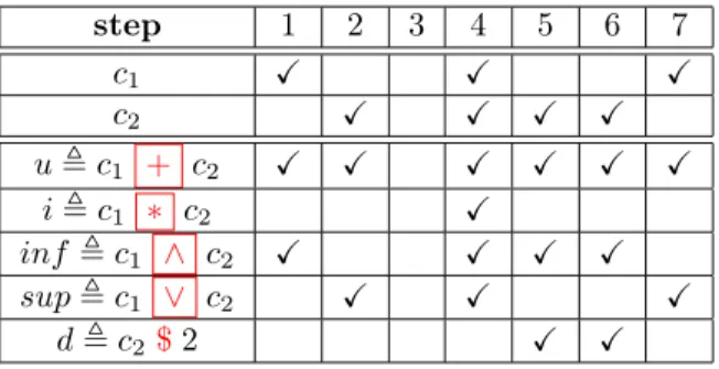
To help the reader understand the semantics of the expressions, Figure 1 gives an example of schedule σ that satisfies several expressions. Check marks represent the steps where a given clock ticks.

3.2

Composition

Definition 12 (CCSL specification satisfaction) A schedule σ satisfies a ccsl specification

SP EC, iff it satisfies all of its constraints: σ |=ccsl SP EC ⇔ (∀rel ∈ Rel, σ |=ccsl rel) ∧ (∀def ∈

step 1 2 3 4 5 6 7 c1 X X X c2 X X X X u , c1 + c2 X X X X X X i , c1 ∗ c2 X inf , c1 ∧ c2 X X X X sup , c1 ∨ c2 X X X d , c2$2 X X

Figure 1: An example of schedule σ

Definition 13 (Bounded CCSL relations) For a given ccsl specification SP EC, a

rela-tion r ∈ Rel is bounded iff (σ |=ccsl SP EC) =⇒ (∃m ∈ N, ∀n ∈ N, |χσ(lef t(r), n) −

χσ(right(r), n)| ≤ m).

Note that, by definition of Causality and because of Proposition 1, we always have op(r) ∈

{ ≺, 4} =⇒ ∀n ∈ N, χσ(lef t(r), n) − χσ(right(r), n) ≥ 0, so we do not have to worry about

finding a lower bound.

Definition 14 (Bounded CCSL expressions) For a given ccsl specification SP EC, a

bi-nary expression e ∈ BinExpr is bounded iff (σ |=ccsl SP EC) =⇒ (∃m ∈ N, ∀n ∈ N, |χσ(f irst(e), n)−

χσ(second(e), n)| ≤ m)). Unary expressions are always bounded.

In [8], we have shown that the behavior of a ccsl specification was captured by the synchro-nized product of the transition systems for each constraint. Obviously, when all the composed transition systems are finite, then the result is necessarily finite. However, the result can also be finite when some of the composed transition systems have an infinite number of states. This is because we only consider the states that are reachable. So safety amounts to having only a finite number of states in the product reachable from the initial state. This is equivalent to being able to bound the counters used in unbounded constraints.

Let us illustrate that on a simple example. Consider, for instance the following ccsl

speci-fication: (c1 ≺ c2) ∧ (c′1 , c1 $ 1) ∧ (c2 ≺ c′1). In this specification, the second constraint

(Delay) is bounded, but the two others are unbounded. However, the result is still considered to be safe since there is only a finite number of reachable states in the synchronized product

as shown in Figure 2. This comes from the fact that counters used in the two Precedences are

bounded by theDelayof the second constraint. This particular composition pattern is frequently

used and is calledAlternation.

s0 s1 s2

hc1i hc2i

hc1, c′1i

Definition 15 (Safe CCSL specification) A ccsl specification is safe iff ∀σ, σ |=ccsl SP EC: • all the relations are bounded: ∀r ∈ Rel, r is bounded,

• all the binary expressions within a clock definition are bounded: ∀e ∈ BinExpr, e is bounded Definition 16 (Bounded precedence) We define a new composite ccsl constraint called Bounded

precedenceby the following satisfaction rule (n ∈ N):

stσ |=ccsl c1 ≺n c2 ⇐⇒ (Boundedprecedence)

σ |=ccsl c1 ≺ c2

∧ σ |=ccsl c′₁, c1$n

∧ σ |=ccsl c2 ≺ c′1

We call alternation the case where n = 1:

σ |=ccsl c1 ∼ c2≡ σ |=ccsl c1 ≺1 c2(Alternation)

Proposition 2 (The bounded precedence is safe) Let c = c1 ≺d c2, constraint c is safe.

Proof of Proposition 2 Let us take a σ such that σ |=ccsl c1 ≺d c2. The first constraint gives

∀n ∈ N, χσ(c1, n) − χσ(c2, n) ≥ 0. The third one gives ∀n ∈ N, χσ(c2, n) − χσ(c′1, n) ≥ 0, so

∀n ∈ N, χσ(c1, n) − χσ(c′1, n) ≥ 0. For the specification to be bounded, we need to show that

∃m ∈ N, ∀n ∈ N, |χσ(c1, n) − χσ(c′1, n)| ≤ m.

If χσ(c1, n) ≤ d, then Eq. 5 gives χσ(c′1, n) = 0 and therefore χσ(c1, n) − χσ(c′1, n) ≤ d.

If χσ(c1, n) ≥ d, then Eq. 5 gives χσ(c′1, n) = χσ(c1, n) − d and also χσ(c1, n) − χσ(c′1, n) ≤ d.

3.3

Safety issues

We consider an abstraction of the ccsl specification that we call acausality clock graph. Indeed,

Causalityis the foundational construct that introduces unbounded integers in a ccsl specification.

Then, we use this abstraction to show that counters included inPrecedence,Causality,Infimumand

Supremumconstraints are bounded. For that purpose, we consider the causal relations includes in a ccsl specification, but we also consider causal relations induced by other constraints. The causality clock graph captures all the causal relations, whether directly specified or induced. The remainder of this subsection discusses the induced causal relations.

Definition 17 (Causality clock graph) A Causality clock graph (CCG) is a directed graph D = (C, A, ∆). C is a set of nodes denoting clocks. A ⊂ C × C is a set of arcs (directed edges). ∆ ⊂ C × C is a set of counter-arcs between two clocks.

In a CCG, an arc a = (c1, c2) is directed from c1 to c2 and denotes a causality c1 4 c2. A

counter-arc δ = (c1, c2) is used to identify a constraint that would generate an infinite number

of states if left unbounded. To each counter-arc δ = (c1, c2), we associate a function δc_c2

1:

δc₂

c₁ : N → N

n 7→ χσ(c1, n) − χσ(c2, n)

The safety analysis must show that for each counter-arc, for each schedule σ, ∃m ∈ nat, ∀n ∈

N_{, |δ}c2

Definition 18 (Complete causality clock graph) Given a ccsl specification SP EC, a

causal-ity clock graph DSP EC is complete with regards to SP EC when all the causal relations implied

by SPEC are captured in the graph and only those relations. ∀σ, σ |=ccsl SP EC, ∀(c1, c2) ∈ C × C,

(∃d ∈ nat, ∀n ∈ N, δc₂

c1(n) ≥ −d ⇔ (c1, c2) is an arc in DSP EC)

The notion of completeness is necessary to show that no causal relation has been ‘forgotten’ in the graph. It means that as soon as a constraint implies that the counter between two clocks can be bounded (either with a lower or an upper bound) then (and only then) there should be a counter-arc in the causality clock graph. Indeed, if arcs are missing, then the safety analysis might conclude that a graph is not safe, while a ccsl specification is actually safe.

3.4

Building the causality clock graph

Obviously, the constraint c1 4 c2always induces a lower bound. For the ccsl specification to be

bounded, we need to establish an upper bound. An arc from c1to c2denotes that we have a lower

bound (∀n ∈ N, δc₂

c₁(n) ≥ 0). A counter-arc between c1 and c2 denotes that we need to establish

the upper bound. More formally, for a given ccsl specification SPEC, we build the causality

clock graph DSP EC = (C, A, ∆) such that ∀r ∈ Rel, op(r) = 4 =⇒ (lef t(r), right(r)) ∈

A ∧ (lef t(r), right(r)) ∈ ∆.

Building arcs only for these relations would lead to an incomplete graph. Other bounds are indeed indirectly induced by most ccsl constraints. The first obvious example is given

by Proposition 1. Hence, every Precedence also leads to an arc and a counter-arc in the CCG.

∀r ∈ Rel, op(r) =≺ =⇒ (lef t(r), right(r)) ∈ A ∧ (lef t(r), right(r)) ∈ ∆.

In the remainder of this section, the other implied causality relations are discussed.

The first family of implications comes from the relationship betweenSubclockingandCausality.

Proposition 3 (Subclocking implies causality) When c1is a subclock of c2then c2is faster

than c1: σ |=ccsl c1 ⊂ c2 =⇒ σ |=ccsl c2 4 c1

Proof of Proposition 3 By recursion on χσ.

HR(n) = χσ(c2, n) ≥ χσ(c1, n). HR(0) is true since χσ(c2, 0) = χσ(c1, 0) = 0. Assume HR(n-1). • If c1 /∈ σ(n)∧c2 /∈ σ(n) then χσ(c1, n) = χσ(c1, n−1)∧χσ(c2, n) = χσ(c2, n−1) then HR(n). • If c1 /∈ σ(n) ∧ c2 ∈ σ(n) then χσ(c1, n) = χσ(c1, n − 1) ∧ χσ(c2, n) = χσ(c2, n − 1) + 1 then HR(n). • If c1 ∈ σ(n) then c2 ∈ σ(n) and χσ(c1, n) = χσ(c1, n − 1) + 1 ∧ χσ(c2, n) = χσ(c2, n − 1) + 1 then HR(n)

Eq. 1a forbids the fourth case.

From Proposition 3, we deduce that we need to build an arc in the CCG from c2to c1 every

time we find a constraint of the form c1 ⊂ c2. However, because this constraint is bounded (see

Definition 13), we do not build any counter-arc in that case.

All the expressions based onSubclocking,i.e.,Union andIntersection, also imply some causality

relations. Here again, the constraints are bounded relations and consequently, no counter-arc is added to the CCG. Let us show these implications.

Proposition 4 (Union and subclocking) A clock is always a subclock of the union of itself

with any other clock: σ |=ccsl u , c1 + c2 =⇒ (σ |=ccsl c1 ⊂ u ∧ σ |=ccsl c2 ⊂ u).

Proof of Proposition 4 Let us assume σ |=ccsl u , c1 + c2.

(c1∈ σ(n) =⇒ (c1∈ σ(n) ∨ c2∈ σ(n)) =⇒ u ∈ σ(n)) =⇒ σ |=ccsl c1 ⊂ u.

(c2∈ σ(n) =⇒ (c1∈ σ(n) ∨ c2∈ σ(n)) =⇒ u ∈ σ(n)) =⇒ σ |=ccsl c2 ⊂ u.

Corollary 1 (Union and causality) The union of two clocks is faster than both clocks:

σ |=ccsl u , c1 + c2 =⇒ (σ |=ccsl u 4 c1∧ σ |=ccsl u 4 c2).

The corollary comes directly from Propositions 3 and 4.

Proposition 5 (Intersection and subclocking) The intersection of two clocks is a subclock

of both clocks: σ |=ccsl i , c1 ∗ c2 =⇒ (σ |=ccsl i ⊂ c1∧ σ |=ccsl i ⊂ c2).

Proof of Proposition 5 Let us assume σ |=ccsl i , c1 ∗ c2.

(i ∈ σ(n) =⇒ (c1∈ σ(n) ∧ c2∈ σ(n)) =⇒ c1∈ σ(n)) =⇒ σ |=ccsl i ⊂ c1.

(i ∈ σ(n) =⇒ (c1∈ σ(n) ∧ c2∈ σ(n)) =⇒ c2∈ σ(n)) =⇒ σ |=ccsl i ⊂ c2.

Corollary 2 (Intersection and causality) The intersection of two clocks is slower than both

clocks: σ |=ccsl i , c1 ∗ c2 =⇒ (σ |=ccsl c1 4 i ∧ σ |=ccsl c2 4 i).

Here again, the corollary comes directly from Propositions 3 and 5.

To be complete, one should also show that Union (resp. Intersection) does not imply any

causality relations between the clocks themselves but only between the union clock u (resp. the

intersection clock i) and the clocks c1and c2. To do so, consider a schedule, where c1 would tick

alone. None of the binary relations can prevent c1 from ticking and thus, the distance between

c1 and c2 can grow infinitely large, thus preventing from having an upper bound. If now, we

consider a schedule were c2ticks alone and c1 never ticks, then such a schedule does not violate

an union or intersection constraint and still prevents us from having a lower bound.

The next step is to determine what causality relations are implied by expressionsInfimumand

Supremum.

Proposition 6 (Infimum and causality) The infimum of two clocks is always faster than

both clocks: σ |=ccsl inf , c1 ∧ c2 =⇒ (σ |=ccsl inf 4 c1∧ σ |=ccsl inf 4 c2).

Proof of Proposition 6 Let us assume σ |=ccsl inf , c1 ∧ c2.

(χσ(inf, n) = max(χσ(c1, n), χσ(c2,n)) =⇒ χσ(inf, n) ≥ χσ(c1, n)) =⇒ σ |=ccsl inf 4 c1.

Similarly, χσ(inf, n) ≥ χσ(c2, n)) =⇒ σ |=ccsl inf 4 c2.

Proposition 7 (Supremum and causality) The supremum of two clocks is always slower

than both clocks: σ |=ccsl sup , c1 ∨ c2 =⇒ (σ |=ccsl c1 4 sup ∧ σ |=ccsl c2 4 sup):

Proof of Proposition 7 Let us assume σ |=ccsl sup , c1 ∨ c2.

(χσ(sup, n) = min(χσ(c1, n), χσ(c2,n)) =⇒ χσ(c1, n) ≥ χσ(sup, n)) =⇒ σ |=ccsl c1 4 sup.

c1

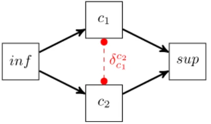
c2

inf δc₂ sup

c₁

Figure 3: Causality Clock Graph for InfimumandSupremum.

The same reasoning as for theUnion andIntersectioncan be used again to show that there is

no causality relation between c1and c2 imposed by eitherInfimumor Supremum. However, these

binary expressions are unbounded (see Definition 14), then we need to add a counter-arc (c1, c2)

in the CCG (see Figure 3). We know that inf is faster than both c1and c2but we need to bound

the counter δc₂

c₁ between c1and c2. Similarly, we know that both c1and c2 are faster than sup.

The last step is to consider the unary expressionDelay.

Proposition 8 (Delay and causality) A clock is always faster than any clock that is delayed

from it: ∀d ∈ N, σ |=ccsl del , c$d =⇒ 0 ≥ δc_del≥ −d

Proof of Proposition 8 If χσ(c, n) ≤ d then Eq. 5 =⇒ χσ(del, n) = 0. Otherwise, χσ(del, n) =

χσ(c, n) − d. In both cases, 0 ≥ δcdel≥ −d.

From Proposition 8, we can deduce that we have both a lower and an upper bound, therefore we must add two arcs: one from c to del and one from del to c. Since the constraint is bounded, no counter-arc must be added in the CCG.

4

A state-based semantics for CCSL operators

This section gives a formal definition of ccsl operators in terms of labeled transition systems. Some of the ccsl operators require an infinite number of states.

4.1

CCSL clocks and relations

Definition 19 (Labeled Transition System) A Labeled Transition System [9] over a set A of actions is defined as a tuple A = hS, T, s0, α, β, λi where

• S is a set of states, • T is a set of transitions, • s0 ∈ S is the initial state,

• α, β : T → S denote respectively the source state and the target state of a transition, • λ : T → A denotes the action responsible for a transition,

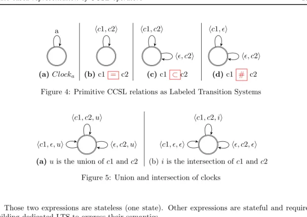
• the mappings hα, λ, βi : T → S × A × S are one-to-one so that T is a subset of S × A × S. In the context of ccsl, the actions are clocks. For each ccsl clock c, we build the Labeled

• S = {s}, T = {t, e}, s0 = s, • α(t) = α(e) = β(t) = β(e) = s, • λ(t) = c and λ(e) = ǫ.

The ǫ action allows for doing nothing. This is to allow composition with other LTSs. Clocka is

given in Figure 4.a as an illustration.2

Definition 20 (Synchronization constraint) Given n sets of actions A1, . . . , An, a

syn-chronization constraintis a subset I of A1× . . . × An.

Definition 21 (Synchronized product) If, for i = 1, . . . , n, Ai= hSi, Ti, s0i,

αi, βi, λii is a labeled transition system over Ai, and if I ⊆ A1× . . . × An is a synchronization

constraint, the synchronized product [9] of Ai with respect to I is the labeled transition system

hS, T, s0, α, β, λi over the set I defined by

• S = S1× . . . × Sn, s0 = s01× . . . × s0n,

• T = {ht1, . . . , tni ∈ T1× . . . × Tn|hλ1(t1), . . . , λn(tn)i ∈ I},

• α(ht1, . . . , tni) = hα1(t1), . . . , αn(tn)i,

• β(ht1, . . . , tni) = hβ1(t1), . . . , βn(tn)i,

• λ(ht1, . . . , tni) = hλ1(t1), . . . , λn(tn)i.

Synchronization constraints allow for capturing the semantics of ccsl polychronous opera-tors. In this section, we focus on ccsl (binary) relations.

Relation 1 (Coincidence) Given two clocks c1 and c2, coincidence c1 = c2 is the

syn-chronized product of Clockc1 and Clockc2 with respect to the synchronization constraint I =

{hc1, c2i, hǫ, ǫi} (Fig. 4.b).

Relation 2 (Subclocking) ccsl subclock (c1 ⊂c2) is the synchronized product of Clockc1

and Clockc2 with respect to the synchronization constraint I = {hc1, c2i, hǫ, c2i, hǫ, ǫi} (Fig. 4.c).

Relation 3 (Exclusion) Figure 4.d illustrates ccsl excludes (c1 # c2) defined as the

syn-chronized product of Clockc1 and Clockc2 with respect to the synchronization constraint I =

{hc1, ǫi, hǫ, c2i, hǫ, ǫi}.

4.2

CCSL bounded expressions

In ccsl, expressions allow for the creation of new clocks based on existing ones. Expressions can also be represented as labeled transition systems. Union and intersection are two simple examples of ccsl expressions.

Expression 1 (Union) u , c1 + c2 (u is the union of c1 and c2) is represented by the

syn-chronized product of Clockc1, Clockc2 and Clocku with respect to the synchronization constraint

I = {hc1, c2, ui, hc1, ǫ, ui, hǫ, c2, ui, hǫ, ǫ, ǫi} (Fig. 5.a).

Expression 2 (Intersection) i , c1.c2 (i is the intersection of c1 and c2) is represented by

the synchronized product of Clockc1, Clockc2 and Clocki with respect to the synchronization

a hc1, c2i hc1, c2i

hǫ, c2i

hc1, ǫi

hǫ, c2i

(a) Clocka (b) c1 = c2 (c) c1 ⊂c2 (d) c1 # c2

Figure 4: Primitive CCSL relations as Labeled Transition Systems

hc1, c2, ui hǫ, c2, ui hc1, ǫ, ui hc1, c2, ii hǫ, c2, ǫi hc1, ǫ, ǫi

(a) u is the union of c1 and c2 (b) i is the intersection of c1 and c2

Figure 5: Union and intersection of clocks

Those two expressions are stateless (one state). Other expressions are stateful and require building dedicated LTS to express their semantics.

Expression 3 (Binary delay) The binary delay (delayed , base $ n) is represented by a

dedicated labeled transition system Delay(n) = hS, T, s0, α, β, λi over A = {init, steady, ǫ} with n + 1 states such that

• S = {d0, d1, . . . , dn}, T = {t0, t1, . . . , tn, e0, . . . , en}, s0 = d0,

• α(ti) = di and α(ei) = di for i ∈ {0 . . . n},

• β(ti) = di+1 for i ∈ {0 . . . n} and β(tn) = dn,

β(ei) = di for i ∈ {0 . . . n},

• λ(ti) = init for i ∈ {0 . . . n − 1} and λ(tn) = steady and λ(ei) = ǫ for i ∈ {0 . . . n}.

init denotes a preliminary phase during which the base clock must tick alone. steady is a phase where both clocks base and delayed become synchronous for ever. Figure 6 gives as an

illustration the resulting transition systems to denote b , a $ 1 (actions init and steady are

hidden).

d0 d1

ha, ǫi

ha, bi

Figure 6: Binary delay: b , a$1

The binary delay is a particular case of a more general synchronous expression called F ilteredBy

(denoted H). f , c H u.(v)ω _{defines the clock f as a subclock of c according to two binary}

words u and v.

2

The ǫ transitions are not shown to simplify the drawings. In all the presented LTSs, it is always possible to do nothing by remaining in the same state.

Definition 22 (Binary word) A binary word w is a function, w : N>0→ {0, 1, ⊥}, such that

(∃l ∈ N>0, w(l) = ⊥) =⇒ ((∀i > l)(w(i) = ⊥)).

Definition 23 (Length of a binary word) If w is a binary word, len(w) (denoted |w|) is

called its length. len : (N>0 → {0, 1, ⊥}) → N ∪ {ω}. If ∀i ∈ N>0, w(i) 6= ⊥ then |w| = ω and

w is said to be an infinite word, otherwise w is a finite word. When w is finite, |w| = min(i ∈

N_{, w(i + 1) = ⊥).}

Definition 24 (Exponentiation of a binary word) Let n be a positive natural number (n ∈ N_{>0). Let v be a finite binary word. w = v}n _{is a finite binary word such that |w| = n ∗ |v| and} ∀i ∈ 1..n, ∀j ∈ {1..|v|}, w(i ∗ j) = v(j).

Definition 25 (Infinitely periodic binary word) Let v be a finite binary word. w = (v)ω _is

an infinite binary word such that ∀i ∈ N, ∀j ∈ {1..|v|}, w(i ∗ |v| + j) = v(j).

Definition 26 (Concatenation of binary words) Let u and v be two binary words, u is fi-nite. w = u.v is a binary word such that (i ≤ |u| =⇒ w(i) = u(i))∧(i > |u| =⇒ w(i) = v(i − |u|)),

∀i ∈ N>0. If v is infinite, then w is infinite. If v is finite, then w is finite and such that

|w| = |u| + |v|.

Expression 4 (Filtering) If u and v are two finite binary words, the LTS for ccsl expression

FilteredByis defined as follows. f , c H u.(v)ω _{is the LTS F ilter(u, v) = hS, T, s0, α, β, λi over}

A = {zero, one, ǫ} with n + 1 states s.t.,

• S = {s1, . . . , s|u|+|v|}, T = {t1, . . . , t|u|+|v|, e1, . . . , e|u|+|v|}, s0 = s1,

• α(ti) = si for i ∈ {1 . . . |u| + |v|},

• β(ti) = si+1 for i ∈ {1 . . . |u| + |v| − 1} and β(t|u|+|v|) = s|u|+1,

• λ(ti) = zero if u(i) = 0 and λ(ti) = one if u(i) = 1, for i ∈ {1 . . . |u|}

• λ(ti+|u|) = zero if v(i) = 0 and λ(ti+|u|) = one if v(i) = 1, for i ∈ {1 . . . |v|}

• α(ei) = si and β(ei) = si and λ(ei) = ǫ for i ∈ {1 . . . |u| + |v|}.

The label one denotes instants where both f and c tick together. The label zero when c

ticks alone. Actually, Delay is just a particular case of filter with u = 0n _{and v = 1. Another}

interesting special case is when u = 0d _{and v = 1.0}p−1_{, for d ∈ N}

>0 and p ∈ N. This defines a periodic pattern P eriodic(d, p), where d is called the offset and p the period. Delay(n) is also a particular periodic case with an offset of n and a period of 1.

Figure 7 gives an example of a periodic filter, where b is periodic on a with a period of 3 and

an offset of 1: b , a H 0.(1.0.0)ω_.

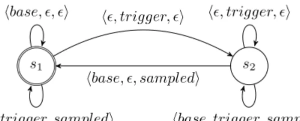
Expression 5 (Sampling) sampled , trigger sampledOn base is the LTS Sampled = hS, T, s0, α, β, λi over A = {base, trig, sample, allǫ} with 2 states such that,

• S = {s1, s2}, T = {b, bs, sa1, sa2, t1, t2, e1, e2}, s0 = s1,

• α(b) = β(b) = s1 and λ(b) = base,

• α(sai) = β(sai) = si and λ(sai) = all for i ∈ {1 . . . 2},

s1 s2 s3 s4

ha, ǫi ha, bi ha, ǫi

ha, ǫi

Figure 7: Example of periodic filter with offset: b , a H 0.(1.0.0)ω

• α(bs) = s2 and β(bs) = s1 and λ(bs) = sample,

• α(ei) = β(ei) = si and λ(ei) = ǫ for i ∈ {1 . . . 2}.

SampledOn is an expression that produces a clock s if and only if a trigger has ticked since the previous tick of a sampling clock (base). Labels base and trig respectively denote instants where clocks base and trigger tick alone. Label sample denotes instants where both clocks base and sampled tick simultaneously. Label all denotes instants where all the three clocks base, trigger and sampled tick simultaneously.

Figure 8 gives the LTS for the sampling operator.

s1 s2

hbase, ǫ, ǫi _{hǫ, trigger, ǫi}

hbase, trigger, sampledi

hbase, ǫ, sampledi

hǫ, trigger, ǫi

hbase, trigger, sampledi

Figure 8: Sampling: sampled , trigger sampledOn base

4.3

Unbounded relations

Unbounded operators can be modeled with labeled transition systems that have an infinite but countable number of states.

Relation 4 (Precedence) Precedence lef t ≺ right is a labeled transition system P recedes =

hS, T, s0, α, β, λi over A = {lef t, right, both, ǫ} s.t.,

• S = {pi|i ∈ N}, T = {li, ri, lri, ei|i ∈ N}, s0 = pi,

• α(li) = α(ei) = α(lri) = pi∧ α(ri) = pi+1, ∀i ∈ N,

• β(li) = pi+1∧ β(ri) = β(ei) = β(lri) = pi, ∀i ∈ N,

• λ(li) = lef t ∧ λ(ri) = right ∧ λ(lri) = both ∧ λ(ei) = ǫ, ∀i ∈ N.

Label lef t denotes instants where clock lef t must tick alone. Label right denotes instants where clock right must tick alone. Label both denotes instants where the two clocks must

tick simultaneously. Figure 9 shows the transition system for the ccsl relation a ≺ b, i.e.,

the synchronized product of Clocka, Clockb and P recedes with respect to the synchronization

constraint I = {ha, ǫ, lef ti, hǫ, b, righti, ha, b, bothi, hǫ, ǫ, ǫi} (lef t, right and both are hidden for the sake of simplicity).

p0 p1 p2 . . .

ha, ǫi ha, ǫi

ha, bi hǫ, bi ha, ǫi ha, bi hǫ, bi ha, bi hǫ, bi

Figure 9: CCSL precedence (infinite state LTS): a precedes b.

This operator is calledunbounded because the drift between a and b is not bounded, i.e., a

can tick infinitely often without b ticking at all. This operator is not symmetrical. Even though a is unconstrained, b on the contrary is constrained to be always a little late compared to a. b is said to be slower than a, or a is faster than b.

4.4

Unbounded expressions

In ccsl, there are two unbounded expressions that constrain neither a nor b: Inf and Sup. Expression 6 (Infimum) Inf (a, b) is the labeled transition system Inf = hS, T, s0, α, β, λi over A = {lef t, right, both, lef t_inf, right_inf, ǫ} such that

• S = {si|i ∈ Z}, T = {inci, deci, ti, ei|i ∈ Z}, s0 = s0,

• α(inci) = α(deci) = α(bothi) = α(ei) = si, ∀i ∈ Z,

• β(bothi) = β(ei) = si and β(inci) = si+1 and β(deci) = si−1, ∀i ∈ Z,

• λ(inci) = lef t_inf if i ≥ 0, and λ(inci) = lef t if i < 0, ∀i ∈ Z

• λ(deci) = right_inf if i ≤ 0, and λ(deci) = right if i < 0, ∀i ∈ Z

• λ(bothi) = both and λ(ei) = ǫ, ∀i ∈ Z

Inf(a, b) is the slowest clock that is faster than both a and b. In most cases, Inf (a, b) is neither a nor b but a clock that sometimes tick simultaneously with a (when a is in advance over b), sometimes it ticks simultaneously with b (when a is late compared to b) and sometimes it ticks simultaneously with a and b (when none of them precedes the other one). Figure 10 shows the transition systems for i , Inf (a, b). This LTS is infinite on both sides. By definition

Inf (a, b) 4 a and Inf (a, b) 4 b, which means that if Inf (a, b) is somehow constrained (i.e.,

by a synchronous operator like filter), then this propagates the constraint on both a and b. Additionally, the tickings of Inf (a, b) are constrained (and bounded) by all the clocks faster than either a or b.

Expression 7 (Supremum) Sup(a, b) is a labeled transition system Sup = hS, T, s0, α, β, λi over A = {lef t, right, both, lef t_sup, right_sup, both_sup, ǫ} such that

s0 s1 . . . s−1 . . . ha, ǫ, ii hǫ, b, ii ha, b, ii ha, ǫ, ii hǫ, b, ǫi ha, b, ii hǫ, b, ǫi ha, b, ii ha, ǫ, ǫi hǫ, b, ii ha, b, ii ha, ǫ, ǫi ha, b, ii

Figure 10: ccsl Inf (infinite state LTS): i , Inf (a, b).

• S = {si|i ∈ Z}, T = {inci, deci, ti, ei|i ∈ Z}, s0 = s0,

• α(inci) = α(deci) = α(bothi) = α(ei) = si, ∀i ∈ Z,

• β(bothi) = β(ei) = si and β(inci) = si+1 and β(deci) = si−1, ∀i ∈ Z,

• λ(inci) = lef t if i ≥ 0, and λ(inci) = lef t_sup if i < 0, ∀i ∈ Z

• λ(deci) = right if i ≤ 0, and λ(deci) = right_sup if i < 0, ∀i ∈ Z

• λ(bothi) = both if i 6= 0 and λ(ei) = ǫ, ∀i ∈ Z, and λ(both0) = both_sup

Sup(a, b) is defined as the fastest clock that is slower than both a and b. In most cases, Sup(a, b) is neither a nor b. Figure 11 shows the transition systems for s , Sup(a, b). By

definition a 4 Sup(a, b) and b 4 Sup(a, b), which means that the constraints imposed on

Sup(a, b) do not directly impact neither a or b. However, whenever a clock c is known to be

slower than either a or b, then it is also slower than Sup(a, b), i.e., (∃c such that a 4 c ∨ b 4

c) =⇒ Sup(a, b) 4 c. s0 s1 . . . s−1 . . . ha, ǫ, ǫi hǫ, b, ǫi ha, b, si ha, ǫ, ǫi hǫ, b, si ha, b, ǫi hǫ, b, si ha, b, ǫi ha, ǫ, si hǫ, b, ǫi ha, b, ǫi ha, ǫ, si ha, b, ǫi

Figure 11: ccsl sup (infinite state LTS): s , Sup(a, b).

5

Boundness issues on CCSL specifications

When several ccsl constraints are put in parallel, the composition is defined as the synchronized product of the LTSs of the operators. However, since some of the LTSs for the primitive operators are infinite (e.g., Relation 4, or Expressions 6-7), the synchronized product might end up being infinite. However, even though the product is potentially infinite, in some cases, only a finite subset of the synchronized product is reachable from the initial state. We show a case where the product of infinite LTSs is finite. The algorithm used in that subsection only terminates when the product is actually finite.

Considering n LTSs such that, for i = 1, . . . , n, Ai = hSi, Ti, s0i, αi, βi, λii and one

synchro-nization constraint I ⊆ A1× . . . × An, the synchronized product of Ai with respect to I is a

labeled transition systemhS, T, s0, α, β, λi over the set I constructed as described in Algorithm

1.

Algorithm 1 Synchronized product through reachability analysis Let S ← ∅, T ← ∅,

Let s0 ← s01× . . . × s0n

Let S′_{← {s0}}

while S’ is not empty {

Let st = st1× . . . × stn be one element of S′

Let S ← S ∪ {st} Let S′_{← S}′_{\ {st}} ∀t = ht1, . . . , tni ∈ T1× . . . × Tn such that (∀i ∈ {1 . . . n})(αi(ti) = sti) and λ1(t1) × . . . × λn(tn) ∈ I { Let st′_{= β} 1(t1) × . . . × βn(tn) if st′_{∈ S then S/} ′_{← S}′_{∪ {st}′_} T ← T ∪ {t}, α(t) = st, β(t) = st′_{, λ(t) = λ} 1(t1) × . . . × λn(tn), } }

Theorem 5.1 Algorithm 1 terminates if and only if the product has a finite number of states.

Proof S′ _{is initialized with one state. At each iteration, one state st is removed from S}′ _and

added to S. All the outgoing transitions of st are computed. If C is the set of clocks, there

are at most 2|C|_{outgoing transitions. Some of these transitions may be inconsistent. For each}

transition the target state st′ _{is computed and added to S}′ _{if not already present in S. This}

condition guarantees that the same state is not visited twice. The algorithm terminates when

S′ _{is empty. S}′ _{becomes empty when all the targeted state are already in S (have already been}

visited). If the set of reachable states is finite then when all the states are in S then S′ _is

necessarily empty. Therefore, when the set of reachable states is finite the algorithm terminates.

If there is an infinite number of reachable states, then S′_{is never empty and the algorithm never}

terminates.

Let us take as an example the following ccsl specification: (a ≺ b)∧(a′_{, a$1)∧(b ≺ a}′_).

This specification is defined as the synchronized product of P recedes (Relation 4), Delay(1) (Expression 3), P recedes (Relation 4 again).

Initially, s0 = p0× d0× p0. The first precedes (state p0) imposes b not to tick, the second

precedes (state p0) prevents a′ from ticking whereas the delay (state d0) only allows a to tick

alone without a′_{. Therefore the only outgoing transition consists in making a ticks alone going}

into the state s1 = p1×d1×p0. At this stage S′ = {s1} and S = {s0}. From s1, the first precedes

(state p1) does not impose any constraint while the second one (state p0) still prevents a′ from

ticking. The delay (state d1) only allows making a and a′ _{tick simultaneously. Since a}′ _cannot

tick, then a cannot tick either, so only b can tick leading to state s2 = p0× d1× p1. Therefore

S = {s0, s1} and S′ _{= {s2}. From s2, the first precedes prevents b from ticking, the second}

relation also prevents b from ticking. The delay only allows a and a′ _{to tick simultaneously.}

Taking this (sole) solution leads to s1, which is already in S, so no new state is added to S′_{. S}′

being therefore empty, the algorithm terminates with S = {s0, s1, s2} (Fig. 12).

This particular construction is very frequent, it has been called Alternation and is denoted

a ∼ b. Increasing the delay from 1 to n makes a particular relation, called bounded

s0 = p0× d0× p0 s1 = p1× d1× p0 s2 = p0× d1× p1

ha, ǫ, ǫi hǫ, b, ǫi

ha, ǫ, a′_i

Figure 12: CCSL alternation: synchronized product of two precedences and one delay

assuming a bound for all ccsl operators, whereas here the bound is computed by reachability analysis. However, the (semi) algorithm sketched above may not terminate when the synchro-nized product is not finite.

6

Example: CCSL for capturing the architecture,

applica-tion and allocaapplica-tion

To illustrate the approach, we take an example inspired by [10], that was used for flow latency

analysis on AADL3

specifications [11]. However, with ccsl we are conducting different kinds of analyses, section 7 discusses some common points with classical real-time scheduling analysis.

6.1

Application

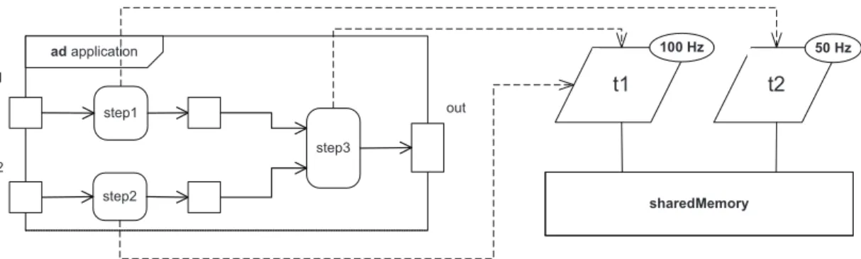
Figure 13 (on the top) considers a simple application described as a uml structured class. This application captures two inputs in1 and in2, performs some calculations (step1, step2 and step3) and then produces a result out. This application has the possibility to compute step1 and step2 concurrently depending on the chosen execution platform. This application runs in a streaming-like fashion by continuously capturing new inputs and producing outputs.

t1 t2 100 Hz 50 Hz ad application step1 step2 step3 sharedMemory in1 in2 out

Figure 13: Simple application

To abstract this application as a ccsl specification, we assign one clock to each action. The clock has the exact same name as the associated action (e.g., step1). We also associate one clock

3

with each input, this represents the capturing time of the inputs, and one clock with the produc-tion of the output (out). The successive instants of the clocks represent successive execuproduc-tions of the actions or input sensing time or output release time. The basic ccsl specification is:

in1 4 step1 ∧ step1 ≺ step3 (6)

in2 4 step2 ∧ step2 ≺ step3 (7)

step3 4 out (8)

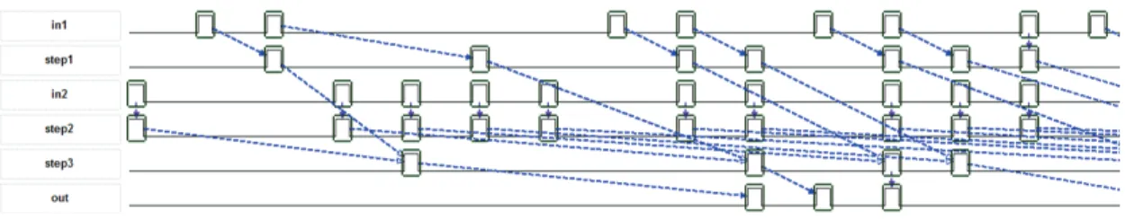
Eq. 6 specifies that step1 may begin as soon as an input in1 is available. Executing step3 also requires step1 to have produced its output. Eq. 7 is similar for in2 and step2. Eq. 8 states that an output can be produced as soon as step3 has executed. Note that ccsl precedence is well adapted to capture infinite FIFOs denoted on the figure as object nodes. Such a specification is clearly unbounded, therefore TimeSquare cannot perform any kind of exhaustive analysis and can only produce a particular schedule that matches the specification (see Fig. 14).

Figure 14: A valid schedule for the application part of Fig. 13

One way to reduce the state-space is to bound the drift between the inputs and the outputs. This means limiting the parallelism by slowing down the production of outputs when several computations are still on-going. This can easily be done by adding a ccsl constraint like Eq. 9.

Sup(in1, in2) ∼ out (9)

The effect of this constraint can be seen on Figure 15. Looking carefully at this schedule, we can note that the arrival of in2 has been slown down to avoid large accumulation of computations. For instance, the third occurrence of in2 is delayed after the second occurrence of out. However, we can see that the input in1 keeps arriving at a fast rate allowing executions of step1. However, the execution of step3 is stalled after the corresponding occurrence of in2 has been dealt with by step2 as required by Eq. 7.

Figure 15: Another valid schedule for the application part of Fig. 13

Reachability analysis as described in Section 5 tells us that the composition is still not bounded because bounds on Sup(in1, in2) do not imply bounds on both in1 and in2. To have

a complete finite systems, we can for instance replace Eq. 9 by Eq. 10.

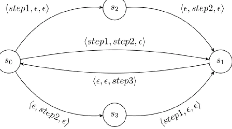
Inf (in1, in2) ∼ out (10)

By doing so, our reachability analysis algorithm converges and produces a bounded

state-space shown in Figure 16 4

. We have removed in1, in2, and out since they were just adding interleaving without offering more actual parallelism in the execution of actions.

s0 s1

s2

s3

hstep1, ǫ, ǫi

hstep1, step2, ǫi

hǫ, st_ep2, ǫi hǫ, ǫ, step3i hǫ, step2, ǫi hstep1 , ǫ,ǫi

Figure 16: Synchronized product of Eqs. 6-8 and Eq. 10.

This kind of analysis is useful to detect invalid ccsl specifications. For instance, had we replaced Eq. 9 by Eq. 11 instead of Eq. 10, we would have obtained a finite result but with a

typical case of deadlock in ccsl. Indeed, if from the initial state s0, we decide to fire in1 (resp.

in2) alone, then Eq. 11 prevents in1+in2 from ticking again before out ticks. But since in2 (resp. in1) was not produced and therefore step2 was not executed, then step3 cannot execute either since it requires both step1 and step2. If step3 cannot execute, then out cannot be produced, which then results in a deadlock.

in1 + in2 ∼ out (11)

6.2

Execution platform and allocation

Once the application is designed, then ccsl can also be used to capture the execution platform. Figure 13 (bottom part) shows the selected execution platform: two tasks with different activation periods. The basic ccsl specification of the execution platform is given as follows:

t1 , ms H (1.09)ω (12)

t2 , t1 H (1.0)ω (13)

Eq. 13 is a pure logical relationship between t1 and t2 that states that thread t2 is twice slower than thread t1, i.e., it is periodic on t1 with period 2 and offset 0. Eq. 12 is also a periodic relation, but relative to ms, a particular clock that denotes milliseconds. Being periodic on ms with a period of 10 makes t1 a 100 Hz clock and therefore t2 a 50 Hz clock.

When the execution platform is specified, the remaining task is to map the application onto the execution platform. In marte, this is done through an allocation. In ccsl, this is done by

4

The algorithm is available as an Eclipse update site on http://timesquare.inria.fr/sts/update_site/

s0 s1

s2

s3

hstep1, ǫ, ǫi

hstep1, step2, ǫi

hǫ, st_ep2, ǫi

hǫ, ǫ, step3i

Figure 17: Synchronous products of Eqs. 6-8 and Eq. 11.

refining the two specifications with new constraints that specify this allocation. Since both step2 and step3 are allocated on the same thread, then their execution is exclusive (Eq. 14). Then, the thread being periodic, the inputs are sampled according to the period of activation of the threads (Eqs. 15-16). Then step3 needs inputs from both step1 and step2 before executing but it can execute only according to the sampling period of t1 since step3 is allocated to t1 (Eq. 17). Finally, all steps can only execute when their input data have been sampled (Eq. 18).

step2 # step3 (14)

in1_s , in1 sampledOn t1 (15)

in2_s , in2 sampledOn t2 (16)

d3_s , Inf(step1, step2) sampledOn t1 (17)

in1_s 4 step1 ∧ in2_s 4 step2 ∧ d3_s 4 step3 (18)

All these new constraints do not change anything on the finiteness of the whole system. They only reduce the set of possible executions. If the application specification was finite, then its allocated version is still finite. If it was infinite, they it remains infinite. Whether it is finite or not, timesquare can produce an execution of this specification (see Fig. 18). On this schedule the dashed arrows denote precedence relations, while the (red) vertical lines denote coincidence relations. Note that the fact that ms is a physical clock does not impact the calculus, it only impacts the visual representation of the schedule.

7

Related work

The transformation of ccsl into labeled transition systems has already been attempted in [12, 13]. However, in those attempts, the ccsl operators were bounded because the underlying model-checkers cannot deal with infinite labeled transition systems. The purpose of this work is to deal with unbounded operators.

In [14], there was an initial attempt to provide a data structure suitable to capture infinite transition systems based on a lazy evaluation technique. A similar structure could be used in our case except that we consider clocks with only two states (instead of three): tick or stall. Clock death is still to be further explored.

Figure 18: A valid schedule for the allocated application (Fig. 13)

The kind of applications addressed in section 6 is very close to models usually used in real-time scheduling theories. However, such theories usually rely on task models that abstract real applications. Originally they were rather simple (e.g., independent periodic tasks only for Rate Monotonic Analysis). Always more sophisticated models now appear in the literature. They are all based on numerous distinct parameters, providing numerical constraint values for timing aspects (dispatch time, period, deadline, jitter drift. . . ). Tasks are considered as iterations of jobs (or jobs as instances of tasks). In our view, the successive timing values for characteristic feature of successive jobs can each be seen as a logical clock, and the time constraint relations between such clocks are usually expressed as simple equalities and bounded inequalities that fall well into the range of ccsl constructs descriptive power.

Classical (non real-time) scheduling, on its side, provides generally models where the initial constraints are less on timing and more on dependencies or on exclusive resource allocation. But

resulting schedules are almost always ofmodulo periodic nature, here again matching the ccsl

expressiveness.

Usually, authors [15, 16, 17] rely on "physical-by-nature" timing, found in theoretical models such as Timed Automata [18]. The distinctive difference is that timed automata assume a global physical time. Timed events are then constrained by value relations between so-called clocks (a different notion from our logical clocks), which are devices measuring physical time as it elapses. Our work also bears some similarity with previous attempts by Alur and Weiss [19, 20], which define schedules as infinite words expressed in regular expressions and then construct corresponding Büchi automata.

8

Conclusion

We have presented a state-based semantics of a kernel subset of ccsl, a language that relies on logical clocks to express logical and temporal constraints. Each ccsl operator (relation or expression) is defined as a label transition system, that may have either a finite or infinite number of states. The parallel composition of ccsl constraints is defined as the synchronized product of the primitive label transition systems. A (semi)algorithm is proposed to actually build the synchronized product of infinite transition systems by assuming that only a finite number of states are accessible in the product. The algorithm only terminates on that condition. The work presented here improves on previous attempts to support exhaustive analyses of ccsl

specifications. Indeed, previous works were only consideringa priori bounded ccsl operators to

guarantee the finiteness of the composition, while here no assumption is made on the boundness of primitive operators.

As a future work, we should extend and prove that data flow process networks can actually be used to detect finite compositions of any unbounded ccsl operators. Whereas it is pretty much clear that synchronous operators and regular asynchronous operators (like precedes, inf, sup) are always covered by synchronous data flow graphs, it is much less clear for mix operators like sampledOn.

References

[1] OMG: UML Profile for MARTE, v1.0. Object Management Group. (November 2009) formal/2009-11-02.

[2] André, C., Mallet, F., de Simone, R.: Modeling time(s). In: 10th Int. Conf. on Model Driven Engineering Languages and Systems (MODELS ’07). Number 4735 in LNCS, Nashville, TN, USA, ACM-IEEE, Springer (September 2007) 559–573

[3] André, C.: Syntax and semantics of the Clock Constraint Specification Language (CCSL). Research Report 6925, INRIA (May 2009)

[4] Deantoni, J., Mallet, F.: Timesquare: Treat your models with logical time. In: TOOLS (50). Volume 7304 of LNCS., Springer (2012) 34–41

[5] Benveniste, A., Caspi, P., Edwards, S.A., Halbwachs, N., Le Guernic, P., de Simone, R.: The synchronous languages 12 years later. Proc. of the IEEE 91(1) (2003) 64–83

[6] Le Guernic, P., Talpin, J.P., Le Lann, J.C.: Polychrony for system design. Journal of

Circuits, Systems, and Computers 12(3) (2003) 261–304

[7] Lee, E.A., Sangiovanni-Vincentelli, A.L.: A framework for comparing models of compu-tation. IEEE Transactions on Computer-Aided Design of Integrated Circuits and Systems 17(12) (December 1998) 1217–1229

[8] Mallet, F., Millo, J.V.: Boundness issues in CCSL specifications. In: ICFEM. Lecture Notes in Computer Science, Springer (2013) to appear.

[9] Arnold, A.: Finite transition systems - semantics of communicating systems. Int. Series in Computer Science. Prentice Hall (1994)

[10] Feiler, P.H., Hansson, J.: Flow latency analysis with the architecture analysis and design language. Technical Report CMU/SEI-2007-TN-010, CMU (June 2007)

[11] of Automotive Engineers, S.: SAE Architecture Analysis and Design Language (AADL). (June 2006) document number: AS5506/1.

[12] Yin, L., Mallet, F., Liu, J.: Verification of MARTE/CCSL time requirements in

Promela/SPIN. In: ICECCS, IEEE Computer Society (2011) 65–74

[13] Gascon, R., Mallet, F., DeAntoni, J.: Logical time and temporal logics: Comparing UML MARTE/CCSL and PSL. In Combi, C., Leucker, M., Wolter, F., eds.: TIME, IEEE (2011) 141–148

[14] Romenska, Y., Mallet, F.: Lazy parallel synchronous composition of infinite transition

systems. In: ICTERI. Volume 1000 of CEUR Workshop Proc. (2013) 130–145

[15] Amnell, T., Fersman, E., Mokrushin, L., Pettersson, P., Yi, W.: Times: A tool for schedula-bility analysis and code generation of real-time systems. In: Formal Modeling and Analysis of Timed Systems. Volume 2791 of LNCS. Springer (2004) 60–72

[16] Krcál, P., Yi, W.: Decidable and undecidable problems in schedulability analysis using timed automata. In: Tools and Algorithms for the Construction and Analysis of Systems. Volume 2988 of LNCS. Springer (2004) 236–250

[17] Abdeddaim, Y., Asarin, E., Maler, O.: Scheduling with timed automata. Theoretical

Computer Science 354(2) (2006) 272–300

[18] Alur, R., Dill, D.L.: A theory of timed automata. Theor. Comput. Sci. 126(2) (1994) 183–235

[19] Alur, R., Weiss, G.: Regular specifications of resource requirements for embedded control software. In: IEEE Real-Time and Embedded Technology and Applications Symp., IEEE CS (2008) 159–168

[20] Alur, R., Weiss, G.: Rtcomposer:a framework for real-time components with scheduling interfaces. In: Int. Conf. on Embedded software. EMSOFT ’08, ACM (2008) 159–168

Contents

1 Introduction 3

2 The Clock Constraint Specification Language 3

3 Definitions 4

3.1 Logical time model . . . 4

3.1.1 Clock relations . . . 5

3.1.2 Clock definitions . . . 6

3.2 Composition . . . 6

3.3 Safety issues . . . 8

3.4 Building the causality clock graph . . . 9

4 A state-based semantics for CCSL operators 11 4.1 CCSL clocks and relations . . . 11

4.2 CCSL bounded expressions . . . 12

4.3 Unbounded relations . . . 15

4.4 Unbounded expressions . . . 16

5 Boundness issues on CCSL specifications 17 6 Example: CCSL for capturing the architecture, application and allocation 19 6.1 Application . . . 19

6.2 Execution platform and allocation . . . 21

7 Related work 22

2004 route des Lucioles - BP 93 BP 105 - 78153 Le Chesnay Cedex inria.fr