HAL Id: hal-00298336
https://hal.archives-ouvertes.fr/hal-00298336
Submitted on 30 May 2007
HAL is a multi-disciplinary open access
archive for the deposit and dissemination of
sci-entific research documents, whether they are
pub-lished or not. The documents may come from
teaching and research institutions in France or
abroad, or from public or private research centers.
L’archive ouverte pluridisciplinaire HAL, est
destinée au dépôt et à la diffusion de documents
scientifiques de niveau recherche, publiés ou non,
émanant des établissements d’enseignement et de
recherche français ou étrangers, des laboratoires
publics ou privés.
Observing the Mediterranean Sea from space: 21 years
of Pathfinder-AVHRR sea surface temperatures (1985 to
2005): re-analysis and validation
S. Marullo, B. Buongiorno Nardelli, M. Guarracino, R. Santoleri
To cite this version:
S. Marullo, B. Buongiorno Nardelli, M. Guarracino, R. Santoleri. Observing the Mediterranean Sea
from space: 21 years of Pathfinder-AVHRR sea surface temperatures (1985 to 2005): re-analysis and
validation. Ocean Science, European Geosciences Union, 2007, 3 (2), pp.299-310. �hal-00298336�
www.ocean-sci.net/3/299/2007/
© Author(s) 2007. This work is licensed under a Creative Commons License.
Ocean Science
Observing the Mediterranean Sea from space: 21 years of
Pathfinder-AVHRR sea surface temperatures (1985 to 2005):
re-analysis and validation
S. Marullo1, B. Buongiorno Nardelli2, M. Guarracino1, and R. Santoleri2
1ENEA, Centro Ricerche Frascati, Via Enrico Fermi 45, 00044 Frascati, Italia
2CNR, Istituto di Scienze dell’Atmosfera e del Clima, Gruppo Oceanografia da Satellite, Via del Fosso del Cavaliere 100,
00133 Roma, Italia
Received: 17 July 2006 – Published in Ocean Sci. Discuss.: 8 August 2006 Revised: 27 April 2007 – Accepted: 13 May 2007 – Published: 30 May 2007
Abstract. The time series of satellite infrared AVHRR data
from 1985 to 2005 has been used to produce a daily series of optimally interpolated SST maps over the regular grid of the operational MFSTEP OGCM model of the Mediter-ranean basin. A complete validation of this OISST (Opti-mally Interpolated Sea Surface Temperature) product with in situ measurements has been performed in order to exclude any possibility of spurious trends due to instrumental cali-bration errors/shifts or algorithms malfunctioning related to local geophysical factors. The validation showed that satel-lite OISST is able to reproduce in situ measurements with a mean bias of less than 0.1 K and RMSE of about 0.5 K and that errors do not drift with time or with the percent interpo-lation error.
1 Introduction
The atmospheric circulation over the Mediterranean area is dominated in winter by the westerlies regime and in sum-mer by the tropical African circulation, that may give rise to subsidence phenomena influencing the Eastern Mediter-ranean basin. These climatic conditions determine large sea surface temperature (SST) excursions between summer and winter, and an important response to the large scale interan-nual variability of the atmospheric forcing over the area. On the other way round, the Mediterranean seasonal predictabil-ity appears to be closely linked to the SST variations, that may produce a feedback through modified heat exchange and transport, and through alterations in the uptake of CO2, with
important implications on both numerical weather prediction and climate research (e.g. Lionello et al., 2006).
Correspondence to: S. Marullo
In addition to the uncertainties related to the natural vari-ability, it is still an open question how deeply the hydrologi-cal cycle of the region has been modified by the intense land usage and coastal urban development in recent years. More-over, as a matter of fact, human activities in the coastal areas and marine resource exploitation, such as open ocean oil ex-traction and industrial fisheries, are experiencing a constant increase, significantly affecting the marine ecosystem.
This large natural variability and the man-induced changes can not be managed without an advanced nowcast-ing/forecasting system. To this aim, the Mediterranean Fore-casting System (MFS) program built up an operational sys-tem for the prediction of currents and biochemical elements in the Mediterranean basin and coastal/shelf areas, developed through a Pilot Project (MFSPP) that lasted from 1999 to 2001, and an advanced project: Towards an Environmen-tal Prediction (MFSTEP), that ended in early 2006. The overall scientific objectives of the program include the mon-itoring and modelling of the ecosystem fluctuations at the level of primary producers and for the time scales of weeks to months, but also a re-analysis of available measurements to explore and better understand the mechanisms driving the Mediterranean dynamics and climate.
To this aim, the SST has been recognized as one of the key parameters: records of SST date back almost one century and satellite observations from infrared data cover now more than 20 years. As a consequence, high resolution/coverage SST data obtained from satellite systems are now available not only for real-time assimilation in forecasting models, but also for interannual/decadal variability studies.
Within the last phase of MFSTEP, a complete re-analysis and interpolation on the MFSTEP OGCM (Ocean General Circulation Model) grid of AVHRR (Advanced Very High Resolution Radiometer) SST measurements from 1985 to
2005 has been performed and is presented here. Interpola-tion of the SST field was required by the presence of data voids in infrared images, due to cloud cover, and to allow simpler assimilation in the numerical models.
As evidenced also by the Global Ocean Data Assimilation Experiment (GODAE) High-Resolution Sea Surface Tem-perature Pilot Project (http://www.ghrsst-pp.org/), interpola-tion is far from being a fully solved problem, and it is still the object of several studies, while many different solutions have already been proposed (e.g. Reynolds et al., 2002; Kaplan et al., 1998; Santoleri et al., 1991). In fact, the algorithms applied may vary due to the different characteristics of the area considered, to the different sources of data and also to numerical limitations.
In this paper, the optimal interpolation scheme developed within MFSTEP is fully detailed. The interpolation scheme was significantly modified with respect to previous MFSPP one (Buongiorno Nardelli et al., 2002), and was used both for the near-real time production of SST maps and for the complete re-analysis of 1985–2005 AVHRR data over the Mediterranean and Eastern Atlantic areas covered by MF-STEP OGCM model grid. The main scope of this work is thus to evaluate the impact of the interpolation algorithm used in the framework of MFSTEP on the accuracy of the SST field, and to assess the accuracy of the re-analyses in order to identify eventual biases that could discourage the application of these data for climate studies (e.g. to detect interannual SST trends in the Mediterranean Sea), or to as-similate data in numerical models. The work clearly required also a further validation of the Pathfinder SST product over the Mediterranean Sea versus in situ data. Though AVHRR instruments sense the temperature of the surface skin layer (SSTskin), the validation has been performed with in situ bulk
data instead of in situ SSTskin data (for a complete
discus-sion on SST definitions see also Donlon et al., 2004). This was coherent with the assumption that our interpolated prod-uct (based only on night-time data) is representative of the so called foundation temperature (SSTfnd, i.e. the SST at the
base of the diurnal heating layer), and gave also the oppor-tunity to go back to 1985 in the validation with a reasonable and nearly uniform amount of matchups. As a result, for the first time a validated time series of 21 years of optimally in-terpolated daily SST fields at high resolution will be available for climatological studies.
The paper is organized as follows: the satellite and in situ data sets are described in Sect. 2. Section 3 is dedicated to the description of the optimal interpolation scheme used. The input data set and interpolated maps validation are presented in Sects. 4 and 5, respectively, while a brief summary and conclusions are discussed in Sect. 6.
2 Satellite and in situ data-set
2.1 Satellite SST
The SST data used in this paper are a Mediterranean subset of the AVHRR Pathfinder product version 5.0. Pathfinder is a joint NASA/NOAA project devoted to the production of global SST maps from 1985 to the present. Pathfinder data are available at daily/4 km time/space resolution, for day and night passes sepa-rately, and are derived from 4-km Global Area Coverage (GAC) data (for more information regarding the version 5 of the Pathfinder data see http://www.nodc.noaa.gov/sog/ pathfinder4km/userguide.html). The Pathfinder algorithm is based on the NLSST (Non Linear Sea Surface Tempera-ture) formulation developed by C. Walton (1988), Walton et al. (1990, 1998a, b) with some modification introduced as a result of the analysis of the PFMDB (PathFinder Matchup Data Base). The NLSST algorithm has the following form: SSTsat=a + bT4+ c (T4−T5)SSTguess+ d (T4−T5) (sec ρ−1)
(1) where SSTsatis the satellite-derived SST estimate, T4and T5
are brightness temperatures in AVHRR channels 4 (10.3 to 11.3 µm) and 5 (11.4 to 12.4 µm) respectively, SSTguessis a
first-guess SST value, and ρ is the satellite zenith angle. Co-efficients a, b, c, and d are estimated from regression analy-ses using co-located in situ and satellite measurements (here-after “matchups”). To reduce the presence of spurious trends in the SST estimates, the PFSST coefficients are estimated on a month by month basis at global scale. Matchups are se-lected within a window of five months, centred on the month for which coefficients were being estimated. This continuous update of the SST algorithm coefficients makes, in principle, the Pathfinder algorithm suitable for studies of year to year SST variability and allows to estimate multi-year SST trends, once the meaning of the used SST has been fixed.
Considering that infrared spacecraft radiometers measure the brightness temperature relative to the skin layer and that Pathfinder SSTs are derived using coefficients based on a re-gression with bulk temperatures, it follows that Pathfinder SST are representative of the SSTskin field minus a “mean
value” of the SSTSkin-SSTbulk temperature difference. In
other words, “the temperature difference between the bulk sensors and the radiating skin is incorporated into the SST retrieval algorithms in an unresolved, statistical sense” (Min-nett, 2003). This statement implies that Pathfinder SST esti-mates taken in conditions that deviate from “mean” can sig-nificantly differ from corresponding in situ bulk measure-ments. This fact is confirmed by recent studies that com-pared satellite estimate to skin measurements rather than bulk measurements (e.g. Kearns et al., 2000; Kumar et al., 2003). They found that, using skin measurements, the scat-ter of the differences between in situ and satellite temper-atures is about half of the corresponding estimate made
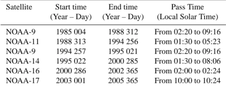
Table 1. Available satellite platforms during the period 1985–2005 and corresponding acquisition time.
Satellite Start time End time Pass Time (Year – Day) (Year – Day) (Local Solar Time) NOAA-9 1985 004 1988 312 From 02:20 to 09:16 NOAA-11 1988 313 1994 256 From 01:30 to 05:23 NOAA-9 1994 257 1995 021 From 02:20 to 09:16 NOAA-14 1995 022 2000 285 From 01:30 to 08:06 NOAA-16 2000 286 2002 365 From 02:00 to 02:24 NOAA-17 2003 001 2005 365 From 10:00 to 10:24
using bulk measurements (RMS about 0.33 K instead of 0.5– 0.7 K). Further details on the processing and algorithms used for SST estimate can be found in the work of Kilpatrick et al. (2001) or in http://www.rsmas.miami.edu/groups/rrsl/ pathfinder/Algorithm/algo index.html.
For this particular work we selected only descending orbits in order to reduce the effect the diurnal cycle on the analy-sis of algorithms and interpolation performances. Table 1 shows local solar time (LST) of the descending passes used for Pathfinder v5.
The Pathfinder SST product includes maps of flags that indicate whether each single SST estimate is contaminated by any environmental factor or not. The flags are obtained throughout a series of tests to assess the likelihood that a pixel contains an SST value of suspect quality. The various tests are then combined to define eight overall quality levels for each pixel (see http://pathfinder.nodc.noaa.gov for a de-tailed description of flags). Of course the best SST estimates are those that have passed all the eight tests. We selected, as valid SST, those pixels that have passed all the tests ex-cluding the reference test (the absolute difference between the Pathfinder SST for the pixel considered and the refer-ence Reynolds SST field must be less or equal to 2 K). This last test has been ignored because another reference test is already included in our OA schema (see Sect. 3.2).
Valid Pathfinder data have been binned on MFSTEP OGCM grid at 1/16◦resolution through a simple median of all valid measurements found within each grid cell. The me-dian was preferred with respect to mean or weighted mean to further reduce the contamination by residual cloudy pixels eventually not flagged.
2.2 In situ data sets
The validation of the OISST time series has been performed with in situ data collected by different sensors, and observa-tional programs. The data used are described in the follow-ing.
2.2.1 MEDAR/MEDATLAS XBT and CTD
MEDAR/MEDATLAS project made available a comprehen-sive data set of oceanographic parameters collected in the Mediterranean and Black Sea, through a wide cooperation of the Mediterranean and Black Sea countries (Fischaut et al., 2002).
Actually, the MEDAR/MEDATLAS data base contains 36 054 CTD casts and 161 890 XBT profiles from about 150 scientific laboratories of 33 countries. These data were sub-mitted to automatic/objective and visual/subjective checks according to international recommendations. As a result, a quality flag is assigned to each numerical value. The list of checks is detailed in the MEDATLAS protocol (http://www. ifremer.fr/sismer/program/medatlas/gb/gb contq.htm).
We selected all the available XBT and CTD profiles cover-ing the Mediterranean Basin from 1 January 1985 to 31 De-cember 2004 excluding those XBT profiles already included in the MFS data base. The MEDATLAS quality control flags were taken into account to select only valid in situ measure-ments for the successive satellite data validation.
2.2.2 MFS XBT
Within the MFS-VOS (MFS-Voluntary Observing Ships) program, an extensive collection of temperature profiles by means of expendable Bathythermographs (XBTs) was started since 1999 in the Mediterranean Sea. The XBT were launched from ships of opportunity along selected tracks crossing the main Mediterranean sub-basins. The uncertainty on XBT temperature values was deeply evaluated by Re-seghetti et al. (20061, 2007) versus simultaneous CTD mea-surements, and was found to be ∼0.10 K (i.e. comparable to the standard accuracy) in the surface layer. All quality controlled MFS-VOS data relative to the period 1999–2005 have been included in our matchup dataset (for a complete description of quality control procedures see Reseghetti et al. (2007)).
1Reseghetti, F., Borghini, M., and Manzella, G. M. R.: Analysis
of XBT data reliability in Western Mediterranean Sea, J. Atmos. Oceanic Technol., submitted, 2006.
2.2.3 MEDARGO floats
A large number of T/S profiles provided by autonomous pro-filers deployed in the Mediterranean is currently available in the framework of the MFSTEP project through CORIOLIS data centre (http://www.coriolis.eu.org/cdc/projects/mfstep. htm). The MEDARGO-MFSTEP program has officially started its operational phase on 13 July 2004 and is still pro-viding data today (Poulain et al., 2006). These floats op-erate at a neutral parking depth of 350 m (near the salinity maximum of the Levantine Intermediate Water) and are pro-grammed to make periodic profiles of temperature and salin-ity from 700 m to surface. The floats reach the surface at intervals of 3–7 days. When at surface, the floats are located by and transmit data to the Argos system onboard the NOAA satellites. The data are processed and archived in near-real time at the CORIOLIS Data Center and are disseminated on the GTS following the standards of the international ARGO program. Temperatures measured by ARGO profilers are ac-curate to ±0.005 K (http://www-argo.ucsd.edu/).
3 The optimal interpolation scheme
3.1 Background
The optimal interpolation (or statistical interpolation) method has been introduced many years ago to determine the optimal solution to the interpolation of a spatially and temporally variable field with data voids, where “optimal” is intended in a least square sense (Gandin, 1965; Bretherton et al., 1976). Its basic principles are quickly reminded in the following. Considering n observations 8obsgiven as the sum
of the “true” value 8 plus a random error ε, and assumed to have known mean <8> and a known and statistically sta-tionary covariance,
8obsi = 8i+ εi
εiεj = δijε2(i, j = 1, . . ., n)
h8i =known (2)
the estimate of 8 at a particular location x (in space and time), is obtained as a linear combination of the observations:
ˆ 8(x) = N X i=1 αi(x)8obsi, (3)
where the coefficients αi are obtained minimizing the error variance. The Gauss-Markov theorem yields solution:
ˆ 8(x) = h8i + n X i=1 n X j =1 A−1ij Cxj(8obsi− h8i), (4)
where the coefficients Cxjand Aijare defined as:
Cxi=(8(x) − h8i)(8obsi − h8i) = F (x, xi) (5)
Aij =(8obsi− h8i)(8obsj− h8i) = Cij+εiεj (6) i.e. they represent the covariance of the field in the obser-vations’ space and the total covariance (signal covariance plus observation error covariance), respectively. In gen-eral, Aij elements (two-points correlations) are computed from a functional fit of the observation covariance values as a function of distance (in our case a “generalized” space-time distance). This approach is called the Observational or Hollingworth-Lonnberg method. Also Cxi can be estimated in this way, taking the zero limit of the observed covariance function at zero distance and exactly the same values else-where.
The method also provides an estimate of the error vari-ance, given by:
D (8(x) − ˆ8x)2 E = Cxx− n X i=1 n X j =1 CxiCxjA−1ij . (7)
All the above is rigorously valid only if it is possible to es-timate the expected value of the field and to remove it from the observations. This is usually done computing an aver-age of the data, and implies that there must be a sufficiently large number of measurements. However, if the expected value cannot be computed as a simple average (example: not enough data), the theory discussed above still leads to a min-imum error variance, provided that a suitable estimated mean is removed from the data. In that case, the coefficients Cxj and Aij represent a structure function and differ from the co-variance function by the unknown constant value <8>2: Cxi =8(x)8obsi = R(x, xi) = F (x, xi) + h8i2
Aij =8obsi8obsj = Cij+εiεj + h8i2 (8) Independently of the value of this constant <8>2, the new estimator is then given by:
ˆ 8(x) = ˜8 + n X i=1 n X j =1 A−1ij Cxj(8obsi− ˜8), (9)
where the estimated mean ˜8 is computed from: n X i=1 n X j =1 A−1ij (8obsi− ˜8) = 0 (10)
i.e. weighting the observations with the observed structure function (Bretherton et al., 1976). This procedure is gener-ally called centering, and the new error estimate includes an additional term: D (8(x) − ˆ8x)2 E = Cxx− n X i=1 n X j =1 CxiCxjA−1ij + 1 − n P i=1 n P j =1 CxiA−1ij !2 n P i=1 n P j =1 Aij . (11)
As Eq. (11) depends on the structure function R, the inter-polation error can be reduced introducing a first guess of the mean field 8g (constant) in the Eqs. (8–11), provided that the new value of Cxx(computed with Eq. (12)) is lower than this obtained through Eq. (8). The structure functions then become:
Cxi=(8(x) − 8g)(8obsi− 8g) =
F (x, xi) − 28gh8i + h8i2= F (x, xi) + H Aij =(8obsi− 8g)(8obsj− 8g) = Cij+εiεj + H
(12) and the new estimator is:
ˆ 8(x) = 8g+ ˜8 + n X i=1 n X j =1 A−1ij Cxj(8obsi− 8g− ˜8) (13)
The estimated mean in that case would obviously be obtained assuming: n X i=1 n X j =1 A−1ij (8obsi− 8g− ˜8) = 0, (14)
while the formula to estimate the error would remain the same as Eq. (11). This last approach has been chosen in MF-STEP, taking as first guess a daily climatological decad field built from the dataset described in Sect. 2.1 but using only those SST values that have passed all quality test (including also the reference test). In practice, each daily climatic map in this first guess field has been computed as the average over the whole 21 years period all the data within a 10 days mov-ing window.
3.2 Description of the interpolation scheme
As the Mediterranean Sea is characterized by the presence of many islands and peninsulas, the scheme drives a “multi-basin” analysis to avoid data propagation across land from one sub-basin to the other. The division of the Mediter-ranean Sea has been performed avoiding the presence of any isolated large island in the sub-basins. As an example, the west Mediterranean has been divided in two parts, one east and one west of the Sardinia and Corsica islands. In math-ematical language each sub-basin is a simply connected do-main. In practice, the optimal interpolation is run several times, one for each sub-basin, applying different masks. Six sub-basin have been identified: Eastern Atlantic, Western Mediterranean basin, Tyrrhenian sea, Adriatic sea, Levantine basin, Aegean sea. In order to avoid artefact effects at the border of the different regions, two different masks are used for each sub-basin, one identifying the interpolation points and one for the selection of the observations. This last in-cludes buffer zones at the borders.
The single analysis scheme includes different modules and its details are described in the following:
Covariance/structure model: it is often unpractical, if not unfeasible in terms of computational time (as in the case of satellite SST data), to use all the data in a series to interpolate the field at a particular time, especially if the dominant scales of variability are shorter than the length of the time series. This is why most of the schemes first compute the covari-ance/structure function from all available data and fit it to an analytical function (implicitly assuming statistical stationar-ity over the whole time series), and successively introduce an
influential radius, which represents the maximum
(general-ized) distance from the interpolation point over which obser-vations are considered useful to the interpolation. In practice, the weights in expression (13) are computed directly from the analytical function, and only for a limited number of obser-vations, reducing significantly the dimensions of the matrix to be inverted, as huge amounts of data in time and space are present in satellite datasets. Here, following the results by Marullo et al. (1999) and our recent researches within the Medspiration project (http://www.medspiration.org) on the main scales of SST variability, a separated dependence of the structure function from time and space lag has been adopted, and the functional form was taken as:
C(r, 1t ) = e−1tτ e− r
L (15)
where r is the relative distance, 1t is the time lag, L=180 km is a sort of spatial ‘decorrelation’ length and τ =7 days is a “temporal” decorrelation scale.
Images selection: the first step in the processing chain in-cludes in the analysis only the images found within a tem-poral window (temtem-poral influential radius) of −10/+10 days with respect to the interpolation day (J ) .
Residual cloudy pixels flagging: successively, three tests are performed on all selected images prior to enter the in-terpolation, in order to avoid contamination by unflagged cloudy pixels. Firstly, cloud margins are eroded, flagging all values within a distance of m pixels to a pixel already flagged as cloudy. The second step consists in rejecting the SST values lower than a minimum threshold SST value (that can be changed seasonally). The third step is the compari-son to the closer (in time) analysis available, that is used as a reference only if the analysis error (as defined in Sect. 3.1) is lower than a fixed value. Data that differ from the reference field for more than a defined threshold (usually 2σ , where σ represents the average standard deviation between consecu-tive night images, estimated as 0.7 K) are not included in the analysis. These “residual cloudy pixels flagging” tests tributed to flag residual clouds and many other partially con-taminated pixels avoiding the use of the Pathfinder reference test that often fails in the Mediterranean Sea in areas where important hot or cold dynamical structures are present. A typical example is the Iera-Petra Gyre in the Levantine basin that most of the time is flagged by the Pathfinder reference test.
First guess removal: coherently to the theory we have de-scribed in Sect. 3.1, the following step consists in the removal
Fig. 1. An example of OISST daily map on 29 December 2000 (a)
and climatological mean of all years (b).
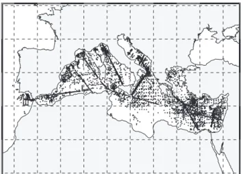
Fig. 2. Spatial distribution of the selected PFSST matchup points.
from each input image of the corresponding decad climato-logical field.
Influential data selection: as already pointed out, for each grid point observations need to be selected within a
space-Fig. 3. Vertical profile of the difference between PFSST and in situ
temperature as function of the depth z.
time influential radius. However, only a sub-set of these observations can effectively be used, because of computa-tional time limitations. In Sect. 3.1, we have seen that the optimal interpolation behaves as a weighted mean of the ob-servations, where the weights are directly related to the corre-lation between the interpocorre-lation point and the single observa-tions, but are reduced if the observations are too much cross-correlated or have low accuracy. Consequently, a strategy to reduce the number of observations in input is to remove most cross-correlated data following some a priori consider-ations. This strategy also reduces numerical problems rais-ing from the inversion of nearly srais-ingular covariance matrices (singularity results from too much cross-correlation). Within MFSTEP, different methodologies have been tried, but very similar results have always been found. The method chosen is a balanced selection around the interpolation point in terms of spatial-temporal coverage, that could be implemented due to the regularity of the grid on which data are organized. The first step thus consists in sorting the data within the influen-tial radius as a function of their correlation to the interpola-tion point. Successively, the most correlated observainterpola-tion is selected (i.e. included in the analysis), while all successive data are selected only if they are found along a new direction in space-time (until 50 observations are found). This allows a more balanced coverage within the influential bubble, even selecting a small number of observations.
Interpolation: the final step is performed estimating the terms Cxjand Aij through the function (15), and the mean of the selected observations through the centering (Eq. 14). Ap-plying the expression (13), the optimal estimate is obtained.
Table 2. Statistical parameters characterizing the differences between in situ SST and Pathfinder data.
MBE RMSE Slope Intercept R n. Pair MEDATLAS-MFS XBT +0.1000 0.4575 0.9982 −0.0641 0.9947 2347 MEDATLAS CTD +0.0743 0.5218 0.9998 −0.0711 0.9930 2469 MEDARGO FLOAT −0.1585 0.7496 0.9930 +0.3110 0.9847 748 ALL DATA +0.0541 0.5400 1.0010 −0.07517 0.9927 5564 10 15 20 25 30 10 15 20 25 PFSS T XBT (C) (a) 10 15 20 25 10 15 20 25 30 CTD (C) MEDARGO (C) (b) (c)
Fig. 4. Scatter plots of PFSST against XBT measurements (a), CTD Measurements (b) and MEDARGO measuremenst (c).
This scheme has been applied to the whole data set from 1985 to 2005. An example of the OISST daily output and the climatological mean of all years are presented in Figs. 1a and b respectively.
4 Evaluation of Pathfinder product in the Mediter-ranean Sea
In order to evaluate the regional performances of the Pathfinder algorithm in the Mediterranean Sea respect to global ocean performances (Kearns et al., 2000; Minnett, 2003), we produced time series of co-located in situ and satellite measurements. Taking into account that in situ ob-servation originates from a variety of sensors with different errors, sensitivity and levels of quality control, we first per-formed the validation separately for each dataset and sensor. More in detail the satellite and in situ match-up dataset was built for MEDATLAS/MEDAR and MFS-VOS XBT, ME-DATLAS/MEDAR CTD and MEDARGO floats.
The space co-location criterion used to build the Mediter-ranean matchup files was set to less than 3.5 km between the measurement point and the centre of the 1/16◦×1/16◦pixel (i.e. the measurement point must fall within the binned satel-lite pixel). Figure 2 shows the spatial distribution of the se-lected matchup points. The time co-location criterion used was simply less than 12 h between satellite and in situ mea-surement.
To be consistent with previous definitions of SSTbulk
(Donlon and the GRHSST science team, 2004) and to limit the effect of the diurnal cycle, for each temperature profile the measurement closer to 3 m depth (in the range 2 m to 6 m depth) was selected. This choice was also supported by the analysis of the difference between temperature T at a given depth z and corresponding PFSST (Fig. 3). The profile has been obtained using all the available matchup data points and averaging the differences at each depth. The absolute value of the mean bias was less than 0.1 K between 2 and 6 m of depth. The minimum absolute difference between PFSST and T (z) was found at a depth of 4 m, where the bias is nearly zero with a standard deviation of 0.6 K. The minimum RMSE (∼0.5 K) was found at 3 m, with a mean bias error close to zero.
Table 2 summarizes the main statistical parameters char-acterizing the difference between in situ and satellite mea-surement for each in situ dataset, and Fig. 4 shows the scatter plots for the three sources of data. The mean depth of the selected temperature was 3.6 m.
The mean bias correction (mean in situ – mean satel-lite) is quite satisfactory and nearly stable for all instru-ments ranging from −0.16 K to 0.10 K. In the following we will use MBE (Mean Bias Error), that usually is expressed as “satellite-in situ”, as synonymous of mean bias correc-tion. The higher differences are found in the comparison with MEDARGO, with a negative MBE of −0.16 K, due to the lack of MEDARGO measurements at depth lower than 4 m (mean reference depth 4.7 m) and coherently with what
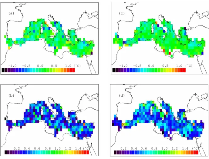
Fig. 5. Spatial distribution of: Tsitu-PFSST (a) and its standard deviation (b); Tsitu-OISST (c) and its standard deviation (d).
found in Fig. 3. The RMSE (standard deviation around the regression line) is very close to 0.5 K for CTD and XBT, while it reaches 0.75 K for MEDARGO. The regression line for XBTs and CTDs basically almost corresponds to the 1 to 1 perfect agreement line. MEDARGO regression line still has a slope very close to 1 but the intersect is 0.3 K.
Averaging all data, the MBE is thus positive but small (+0.05 K) due to the relative little amount of MEDARGO data with respect to the sum of XBT and CTD measurements (about 16% of the total). The RMSE values are anyway very close to previous estimates obtained from global data (e.g. Strong and McClain, 1984).
If MEDARGO data are not included in the analysis, the MBE reaches 0.08 K, a value very close to previous global estimates. In fact, differences between PFSST and in situ SSTskinat night are expected to be 0.1±0.33 K for mid- and
low-latitudes (Kearns et al., 2000; Minnett, 2003) .
Figures 3 and 6 by Minnett (2003) show that the mean dif-ference between SSTskinand SST3 mvaries depending on the
true wind speed intensity, but this difference is, in general, around −0.2 K at night, in most of the cases independently from the wind intensity.
(For night passes) PFSST – SSTSkin∼0.1 K
(after Kearns et al., 2000)
(For Night measures) SSTSkin– SST3 m∼−0.2 K
(after Minnett, 2003)
It follows that, on average at mid- and low-latitudes, the difference between SST3 m and PFSST should be about
0.1 K, which is not so far from the results found. This is also in agreement with previous estimates of Pathfinder perfor-mances in the Mediterranean Sea made using an old version of Pathfinder algorithm for the years 1985–1994 (D’Ortenzio et al., 2000).
In the following, considering the uniform behaviour of the available source of data (see Table 2), we will continue our analysis using all the data as a single dataset.
The spatial distribution of the in situ and satellite temper-ature difference (Fig. 5a) and its standard deviation (Fig. 5b) is quite uniform and generally positive with few hot spots greater then 0.5 K mostly located near the coasts.
First of all we evaluate the monthly behaviour of the dif-ference between in situ and satellite estimate in order to ver-ify whether a seasonal signal was present or not. Figure 6b
10 15 20 25 30 10 15 20 25 30 OISST (˚C) Tsitu (˚C) 10 15 20 25 30 10 15 20 25 30 PFSST (˚C) Tsitu (˚C) 2 3 4 6 1 5 7 8 9 10 11 12 Month 0.0 0.5 -0.5 1.0 1.5 -1.0 -1.5 2 3 4 6 1 5 7 8 9 10 11 12 Month 0.0 0.5 -0.5 1.0 1.5 -1.0 -1.5 Tsitu-OISST 1985 1990 1995 2000 2005 YEAR 0.0 0.5 -0.5 1.0 1.5 -1.0 -1.5 1985 1990 1995 2000 2005 YEAR 0.0 0.5 -0.5 1.0 1.5 -1.0 -1.5 Tsitu-PFSST Tsitu-OISST
(a)
(c)
(e)
(f)
(d)
(b)
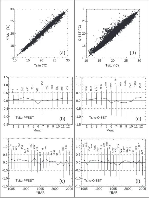
Tsitu-PFSSTFig. 6. Comparison of PFSST and OISST behaviour against in situ observations: scatterplot Tsitu versus PFSST (a), monthly behaviour of
Tsitu-PFSST (b), yearly behaviour of Tsitu-PFSST (c), scatterplot Tsitu versus OISST (d), monthly behaviour of Tsitu-OISST (e), yearly behaviour of Tsitu-OiSST (f). Vertical bars represent the standard deviation of the differences and the numbers represent the number of matchups for each mean.
shows the mean monthly values of the bias between in situ measurements and satellite estimates. The MBE ranges from −0.17 K in June to +0.17 K in December with standard devi-ations comprised between 0.30 K in February and 0.84 K in
July. The tendency of the MBE to zero or to a slightly nega-tive values during the warmer months (May, June, July, Au-gust and September) indicates the presence of a very small seasonal signal. This is not surprising, even though the
Fig. 7. Spatial distribution of the selected OISST matchup points.
Pathfinder SST uses temporally varying coefficients in the at-mospheric correction algorithm; but the application of these globally optimized coefficients in a regionally-constrained study could likely lead non-zero bias errors (Minnett, 1990). The behaviour of the yearly MBE permits to evaluate satellite eventual sensor drifts or shifts that could prevent the use of Pathfinder SST data to evaluate trends in the SST of the Mediterranean Sea for the period 1985–2005. Figure 6c shows that the MBE does not significantly decrease/increase with years exhibiting a slope of −0.01±0.02 K/year (the standard deviations of each mean difference have been used to estimate the uncertainty for the slope).
5 Validation of two decades of OISST
OISST maps were validate against in situ data using the same procedure applied in Sect. 4 for PFSST. The process pro-duced a total of more than 21 000 matchups which spatial dis-tribution is shown in Fig. 7. Table 3 shows the main statistical parameters that describe the differences between in situ mea-surements and Optimally Interpolated SST (OISST). These statistical parameters are very similar to those of Tinsitu
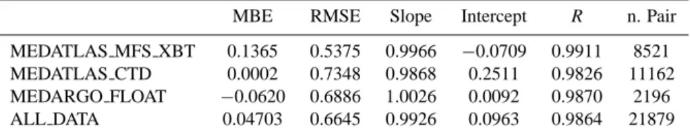
-PFSST (Table 2). The mean difference between XBT mea-surements and OISST estimates remains more or less the same moving from 0.10 K to 0.14 K. For CTD the MBE be-comes slightly better than the previous value of 0.07 K. In the case of MEDARGO floats the MBE is now closer to zero reaching the value of −0.06 K.
Also the RMSE does not significantly change, even if a slight increase from 0.52 K to 0.73 K is observed in the case of CTD data and decrease from 0.75 K to 0.69 K is ob-served for MEDARGO floats resulting in an overall RMSE of 0.66 K. Slopes and intercepts as well as correlation coeffi-cients remain basically unchanged. The scatter plot of in situ measurement against OISST is shown in Fig. 6d.
Tsitu-OISST
% OI Error
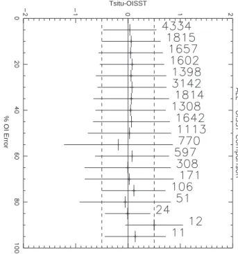
Fig. 8. Behaviour of Tsitu-OISST as a function of the OI
interpo-lation error. Vertical bars represent the standard deviation of the differences and the numbers represent the number of matchups for each mean.
The behaviour of the SSTinsitu-OISST on monthly and
yearly basis is shown in Figs. 6e and f respectively. A first comparison with the corresponding figures obtained using PFSST (Figs. 6b and c) instead of OISST indi-cates that the OISST have not introduced significant dif-ferences and that the main characteristics of the behaviour remained unchanged. The use the MBE does not signif-icantly decrease/increase with years, exhibiting a slope of 0.00±0.02 K/year (the standard deviation of each mean dif-ference have been used to estimate uncertainty for the slope). The MBE ranges from −0.14 K in June to +0.20 K in De-cember with standard deviations comprised between 0.36 K in March and 0.96 K in July. The tendency of the MBE to slightly negative values during the warmer months (June, July, August and October) indicates the presence of a very small seasonal signal similar to that already contained in the PFSST MBE time series.
Another interesting feature of the OISST estimates is the behaviour of the MBE and RMSE as a function of the in-terpolation error. Figure 8 indicates that the MBE is essen-tially constant and very close to zero for interpolation errors less or equal 50%. For interpolation errors greater than this value, but less than 85% SSTinsitu-OISST ranges in the
in-terval −0.19 K to 0.08 K. For interpolation errors greater or equal 90% the MBE reaches values as high as 0.5 K but, in this case the number of matchup points is very small (only 12 matchups for 90% error and 11 for 95% error).
Table 3. Statistical parameters characterizing the differences between in situ SST and OISST data.
MBE RMSE Slope Intercept R n. Pair MEDATLAS MFS XBT 0.1365 0.5375 0.9966 −0.0709 0.9911 8521 MEDATLAS CTD 0.0002 0.7348 0.9868 0.2511 0.9826 11162 MEDARGO FLOAT −0.0620 0.6886 1.0026 0.0092 0.9870 2196 ALL DATA 0.04703 0.6645 0.9926 0.0963 0.9864 21879
Concerning the spatial distribution of the SSTinsitu and
OISST difference (Fig. 5c) and its standard deviation (Fig. 5d) only minor differences with respect to the patterns seen for PFSST are found, with a slightly higher RMSE along the western coasts of the Italian peninsula (Tyrrhenian and Ligurian Sea) and South coasts of France.
6 Summary and conclusion
Among the priorities of the Global Ocean Data Assimilation Experiment, it was clearly indicated the necessity to have an accurate and systematic estimate of the SST at high spa-tial resolution and daily repetitivity, mainly based on satel-lite measurements, with no data voids, at global and regional scales. These requirements were driven both by climatolog-ical researches and by operational applications, with the fi-nal objective of monitoring, understanding and managing the natural variability and the man-induced changes to the ma-rine ecosystem.
Within the MFSTEP program, an optimally interpolated SST product covering the Mediterranean and Eastern At-lantic area at 1/16◦resolution has been developed and pro-duced in near-real-time for direct assimilation in MFSTEP large scale model. The hypothesis and assumptions behind MFSTEP optimal interpolation scheme have been fully de-scribed in this paper, detailing the characteristics of each module (from cloud detection to data selection, etc.) and jus-tifying authors’ choices in the light of theoretical and practi-cal considerations.
The algorithm presented was then used to perform a re-analysis of Pathfinder SST time series, dating back to 1985. In fact, the main scope of the work was to evaluate the im-pact of MFSTEP interpolation scheme on the accuracy of the SST field, and to validate the 1985–2005 OISST time series. Comparing OISST and original Pathfinder SST data (that were used as input data for the OI) with simultaneous MEDAR/MEDATLAS, MFS-VOS and MEDARGO mea-surements, it was possible to estimate the OISST accuracy in terms of mean bias error and standard deviation with re-spect to the SST nearest to 3 m of depth (in the layer 2 m– 6 m, see Sect. 4), assumed here as the best approximation to the foundation temperature. The results indicated that the impact of the OI is quite limited, with an increase in the
RMSE from 0.54 K to 0.66 K and even a slightly better MBE (around 0.04 K). Moreover, the sensitivity of both PFSST and OISST accuracy to seasonal factors has been evaluated to be lower than 0.3 K and, even more importantly, the presence of significant sensor drifts, shifts or responses to anomalous atmospheric events could be excluded by the present anal-ysis. An other interesting result is that the actual statistics of the satellite SST errors varies to some degree on the data set being used to validate the satellite retrievals (XBT, CTD and MEDARGO floats). This may be caused by the way the different validating data sets sample the oceanic and at-mospheric variability, but it could be that the contribution of the error statistics from uncertainties in the validating data is non-negligible. This means that the satellite data are more accurate than these, and other, results indicate.
As a conclusion, the MFSTEP OISST produced by the re-analysis of the PFSST represent a valuable dataset to investi-gate interannual and decade-to-decade variability of the SST field, to detect trends and anomalously warm/cold years (e.g. 2003) and to investigate the role of local and remote forcing, also through assimilation in numerical models.
Acknowledgements. This study was funded by Mediterranean
Forecasting Towards Environmental Predictions (MFSTEP) and by Marine and EnviRonment and Security for European Area (MERSEA) European integrated projects. NODC/RSMAS AVHRR Pathfinder Version 5 SST data were obtained from NODC at the NASA Physical Oceanography Distributed Active Archive Center (PO.DAAC) (http://podaac-www.jpl.nasa.gov/sst/). The authors also sincerely thank P. Minnett and K. Casey for the helpful comments on this article.
Edited by: N. Pinardi
References
Bretherton, F. P., Davis, R. E., and Fandry, C. B.: A technique for objective analysis and design of oceanographic experiments ap-plied to MODE-73, Deep Sea Res., 23, 559–582, 1976. Buongiorno Nardelli, B., Larnicol, G., D’Acunzo, E., Santoleri, R.,
Marullo, S., and Le Traon, P. Y.: Near Real Time SLA and SST products during 2-years of MFS pilot project: processing, analy-sis of the variability and of the coupled patterns, Ann. Geophys., 20, 1–19, 2002,
Donlon, C. J., Minnett, P. J., Gentemann, C., Nightingale, T. J., Barton, I. J., Ward, B., and Murray, J.: Towards improved vali-dation of satellite sea surface skin temperature measurements for climate research, J. Climate, 15, 353–369, 2002.
Donlon, C. J. and the GHRSST-PP Science Team: The Recom-mended GHRSST-PP Data Processing Specification GDS (Ver-sion 1 revi(Ver-sion 1.5), GHRSST-PP Report Number 17. Published by the International GHRSST-PP Project Office, UK Met Office, United Kingdom, 235 pp., 2004.
D’Ortenzio, F., Marullo, S., and Santoleri, R.: Validation of AVHRR Pathfinder SST’s over the Mediterranean Sea, Geophys. Res. Lett., 27, 2, 241–244, 2000.
Fichaut, M., Garcia, M.-J., Giorgetti, A., Iona, A., Kuznetsov, A., Rixen, M., and Group, M.: MEDAR/MEDATLAS 2002: A Mediterranean and Black Sea database for the operational Oceanography, in: Building the European Capacity in Opera-tional Oceanography: Proceedings 3rd EuroGOOS Conference, edited by: Dahlin, H., Flemming, N. C., Nittis, K., and Petersson, S. E., Elsevier Oceanogr. Ser., 69, 645–648, 2002.
Gandin, L. S.: Objective analysis of meteorological fields, Israel Program for Scientific Translation, Jerusalem, pp. 242, 1965. Kilpatrick, K. A., Podesta, G. P., and Evans, R.: Overview of
the NOAA/NASA Advanced Very High Resolution Radiometer Pathfinder algorithm for sea surface temperature and associated matchup database, J. Geophys. Res.-Oceans, 106(C5), 9179– 9197, 2001.
Kaplan, A., Cane, M. A., Kushnir, Y., Clement, A. C., Blumenthal, M. B., and Rajagopalan, B.: Analyses of global sea surface tem-perature 1856–1991, J. Geophys. Res., 103(C9), 18 567–18 590, doi:10.1029/98JC01736, 1998.
Kearns, E. J., Hanafin, J. A., Evans, R. H., Minnett, P. J., and Brown, O. B.: An independent assessment of Pathfinder AVHRR sea sur-face temperature accuracy using the Marine-Atmosphere Emit-ted Radiance Interferometer (M-AERI), B. Am. Meteorol. Soc., 81, 1525–1536, 2000.
Kumar, A., Minnett, P. J., Podesta, G., and Evans, R. H.: Error characteristics of the atmospheric correction algorithms used in retrieval of sea surface temperatures from infrared satellite mea-surements; global and regional aspects, J. Atmos. Sci., 60, 575– 585, 2003.
Lionello, P., Malanotte-Rizzoli, P., and Boscolo, R.: The Mediter-ranean climate: an overview of the main characteristics and is-sues, Elsevier, Amsterdam, Netherlands, 2006.
Marullo, S., Santoleri, R., Rizzoli, P. M., and Bergamasco, A.: The Sea Surface Temperature Field in the Eastern Mediterranean from AVHRR data. Part I. Seasonal variability, J. Mar. Syst., 20, 63–81, 1999.
Minnett, P. J.: The regional optimization of infrared measurements of sea-surface temperature from space, J. Geophys. Res, 95, 13 497–13 510, 1990.
Minnett, P. J.: Radiometric measurements of the sea-surface skin temperature: the competing roles of the diurnal thermocline and the cool skin, Int. J. Rem. Sens., 24, 24, 5033–5047, 2003. Poulain, P.-M., Barbanti, R., Font, J., Cruzado, A., Millot, C.,
Gertman, I., Griffa, A., Rupolo, V., Le Bras, S., and Petit de la Villeon, L.: MEDARGO: A Profiling Float Program in the Mediterranean Sea Ocean Sciences, Ocean Sci. Discuss., 3, 1901–1943, 2006,
http://www.ocean-sci-discuss.net/3/1901/2006/.
Reseghetti, F., Borghini, M., and Manzella, G. M. R.: Factors af-fecting the quality of XBT data – results of analyses on pro-files from the Western Mediterranean Sea, Ocean Sci., 3, 59–75, 2007,
http://www.ocean-sci.net/3/59/2007/.
Reynolds, R. W., Rayner, N. A., Smith, T. M., Stokes, D. C., and Wang, W.: An improved in situ and satellite SST analysis for climate, J. Climate, 15, 1609–1625, 2002.
Santoleri, R., Marullo, S., and Bohm, E.: An Objective Analysis Schema for AVHRR Imagery, Int. J. Rem. Sens., 12, 681—93, 1991.
Strong, A. E. and McClain, E. P.: Improved ocean surface tem-peratures from space – comparisons with drifting floats, B. Am. Meteorol. Soc., 65, 138–142, 1984.
Walton, C. C., Pichel, W. G., Sapper, J. F., and May, D. A.: The development and 5046 P. J. Minnett operational application of nonlinear algorithms for the measurement of sea surface temper-atures with the NOAA polar-orbiting environmental satellites, J. Geophys. Res., 103, 27 999–28 012, 1998.
Walton, C. C., McClain, E. P., and Sapper, J. F.: Recent changes in satellite based multichannel sea surface temperature algo-rithms, Marine Technology Society Meeting, MTS’ 90, Wash-ington D.C., September 1990.
Walton, C. C., Pichel, W. G., Sapper, J. F., and May, D.: The development and operational application of nonlinear algo-rithms for the measurement of sea surface temperatures with the NOAA polar-orbiting environmental satellites, J. Geophys. Res., 103(C12), 27 999–28 012, 1998a.
Walton, C. C., Sullivan, J. T., Rao, C. R. N., and Weinreb, M.: Cor-rections for detector nonlinearities and calibration inconsisten-cies of the infrared channels of the advanced very high resolution radiometer, J. Geophys. Res., 103(C2), 3323–3337, 1998b.