HAL Id: hal-00296317
https://hal.archives-ouvertes.fr/hal-00296317
Submitted on 22 Aug 2007
HAL is a multi-disciplinary open access
archive for the deposit and dissemination of
sci-entific research documents, whether they are
pub-lished or not. The documents may come from
teaching and research institutions in France or
abroad, or from public or private research centers.
L’archive ouverte pluridisciplinaire HAL, est
destinée au dépôt et à la diffusion de documents
scientifiques de niveau recherche, publiés ou non,
émanant des établissements d’enseignement et de
recherche français ou étrangers, des laboratoires
publics ou privés.
Sensitivity of PM2.5 to climate in the Eastern US: a
modeling case study
J. P. Dawson, P. J. Adams, S. N. Pandis
To cite this version:
J. P. Dawson, P. J. Adams, S. N. Pandis. Sensitivity of PM2.5 to climate in the Eastern US: a
modeling case study. Atmospheric Chemistry and Physics, European Geosciences Union, 2007, 7 (16),
pp.4295-4309. �hal-00296317�
www.atmos-chem-phys.net/7/4295/2007/ © Author(s) 2007. This work is licensed under a Creative Commons License.
Chemistry
and Physics
Sensitivity of PM
2.5
to climate in the Eastern US: a modeling case
study
J. P. Dawson1,2, P. J. Adams2,3, and S. N. Pandis1,4
1Department of Chemical Engineering, Carnegie Mellon University, 5000 Forbes Ave., Pittsburgh, Pennsylvania 15213, USA 2Department of Engineering and Public Policy, Carnegie Mellon University, 5000 Forbes Ave., Pittsburgh, Pennsylvania 15213, USA
3Department of Civil and Environmental Engineering, Carnegie Mellon University, 5000 Forbes Ave., Pittsburgh, Pennsylvania 15213, USA
4Department of Chemical Engineering, University of Patras, 26500, Patra, Greece
Received: 14 February 2007 – Published in Atmos. Chem. Phys. Discuss.: 14 May 2007 Revised: 13 August 2007 – Accepted: 16 August 2007 – Published: 22 August 2007
Abstract. The individual effects of various
meteorologi-cal parameters on PM2.5 concentrations in the Eastern US are examined using the PMCAMx chemical transport model so that these effects and their relative magnitudes can be better understood. A suite of perturbations in temperature, wind speed, absolute humidity, mixing height, cloud cover, and precipitation are imposed individually on base case con-ditions corresponding to periods in July 2001 and January 2002 in order to determine the sensitivities of PM2.5 con-centrations and composition to these separate meteorolog-ical parameters. Temperature had a major effect on av-erage PM2.5 in January (−170 ng m−3K−1)due largely to the evaporation of ammonium nitrate and organic aerosol at higher temperatures; increases in sulfate production with increased temperature counteracted much of this decrease in July. Changes in mixing height also had major ef-fects on PM2.5concentrations: 73 ng m−3(100 m)−1in Jan-uary and 210 ng m−3 (100 m)−1 in July. Changes in wind speed (30 to 55 ng m−3%−1) and absolute humidity (15 to 20 ng m−3%−1)also had appreciable effects on average PM2.5 concentrations. Precipitation changes had large im-pacts on parts of the domain (a consequence of the base case meteorology), with sensitivities to changing area of pre-cipitation in July up to 100 ng m−3%−1. Perturbations in cloud cover had the smallest effects on average PM2.5 con-centrations. The changes in PM2.5 concentrations resulting from changing all eight meteorological parameters simulta-neously were approximately within 25% or so of the sum of the changes to the eight individual perturbations. The sen-sitivities of PM2.5 concentrations to changes in these mete-orological parameters indicate that changes in climate could potentially have important impacts on PM2.5concentrations.
Correspondence to: S. N. Pandis ([email protected])
1 Introduction
High concentrations of particulate matter (PM), a major con-stituent of air pollution, have detrimental effects on human health (Godish, 2004). Particulate air pollution has been as-sociated with increases in mortality (Schwartz et al., 1996) and can aggravate respiratory and cardiovascular diseases, damage lung tissue, and lead to premature death (Bernard et al., 2001). The health effects of particulate matter have been associated with both short- and long-term exposure (Kappos et al., 2004).
Concentrations of PM are strongly influenced by mete-orology, but there has been little research on how con-centrations depend on individual meteorological parameters (Elminir, 2005). PM is comprised of many different species, and meteorology can have complex effects on total PM con-centrations due to its impacts on individual species. Aerosol sulfate concentrations depend on the temperature-dependent oxidation of SO2in both the gas and aqueous (cloud) phases (Seinfeld and Pandis, 2006). The concentrations of oxidants that react with SO2 are also dependent on temperature and sunlight intensity (Sweet and Gatz, 1998). Concentrations of semi-volatile nitrate and organic aerosols are temperature and relative humidity dependent; they can also vary with the amount of oxidants present, which is linked to photolysis rates and, therefore, cloud cover. All species have wet de-position as a major sink, so precipitation is expected to have a significant effect on aerosol concentrations. Finally, mix-ing and dilution influence PM concentrations, so wind speed and mixing height are expected to have an impact as well.
Emissions control policy is currently made assuming that climate will remain constant. However, climate changes over the next decades are expected to be significant and may im-pact PM concentrations; for example, global average temper-atures are expected to rise 1.5 to 4.5 K over the next century
2.5
(IPCC, 2001). Predictions of wind speed changes in the United States vary depending on the area in question and on the model used. Bogardi and Matyasovszky (1996) predict spatially variable changes in wind speeds in Nebraska un-der a future climate. Breslow and Sailor (2002) predict wind speed decreases over the United States in the next 50 years. Absolute humidity (water vapor concentration) is generally expected to increase due to the higher saturation vapor pres-sure of water at higher temperatures (IPCC, 2001). Held and Soden (2000) point out that many models predict that future relative humidity will remain roughly constant with climate change. Norris (2005) has observed decreases in cloud cover in recent decades over most of the planet. Simulations us-ing general circulation models (GCMs) indicate that cloud cover decreases when temperature increases (Cess et al., 1990). GCM studies also predict minor changes in summer and annual mean precipitation over the eastern United States (R¨ais¨anen, 2005). Leung and Gustafson (2005), however, predict significant changes in the number of summer days with precipitation in the Eastern USA. Mickley et al. (2004) and Hogrefe at al. (2004) report increased mixing heights in future climates, though Murazaki and Hess (2006) predict no significant changes in mixing heights in a future climate.
While the response of ozone to changes in meteorology and climate has been examined (Hogrefe et al., 2004; Daw-son et al., 2007; Baertsch-Ritter et al., 2004; Racherla and Adams, 2007; Johnson et al., 2001; Brasseur et al., 1998, 2006; Unger et al., 2006; Liao et al., 2006; Muraraki and Hess, 2006; Steiner et al., 2006), there has been relatively little work connecting aerosol concentrations and meteorol-ogy. The corresponding studies have generally been statisti-cal observational studies (Elminir, 2005; Wise and Comrie, 2005; Triantafyllou et al., 2002), along with a small number of modeling studies (Unger et al., 2006; Liao et al., 2006). These studies illustrate the difficulty in deriving causal re-lationships between specific meteorological parameters and measured PM concentrations when the meteorological vari-ables are strongly correlated with one another.
A few process modeling studies have also looked at the connections between meteorology and aerosol concentra-tions. The results of Mickley et al. (2004) suggest (us-ing black carbon as a tracer) that a warmer future climate could increase the severity of summertime PM episodes in the Northeastern and Midwestern USA. Racherla and Adams (2007) predicted decreases in global burdens and lifetimes of fine PM using the IPCC A2 scenario, though global-average changes at the surface level were small and regional re-sponses were mixed. Increases in aerosol sulfate over the eastern USA were also suggested by this work. In a study that includes both observation and process modeling com-ponents, Koch et al. (2003) observed a significant negative correlation between cloud cover and aerosol sulfate due to the longer lifetime of gas-phase-produced sulfate compared to aqueous-phase-produced sulfate. Aw and Kleeman (2003) calculated decreases in PM2.5 concentrations due to
tem-perature increases in a modeling study over southern Cali-fornia; this was due to decreases in semi-volatile aerosols, especially ammonium nitrate. The same study predicted increases in non-volatile PM concentrations with tempera-ture. Using a box model, Sheehan and Bowman (2001) pre-dicted an increase in secondary organic aerosol (SOA) yields of 20–150% for a 10 K decrease in temperature due to the temperature-dependent partitioning of the aerosol.
Determining how PM concentrations change as climate changes is an important step toward estimating future air quality. This may allow air quality policy planners to re-lax the assumption of constant climate and meteorology, or it may indicate that the assumption of constant climate will have little effect on predicted air quality. Observational stud-ies have generally focused on small areas (e.g. one city) and have difficulties in separating the effects of different atmo-spheric variables; the response of PM concentrations over large regions has been the focus of little research. Addition-ally few studies have calculated sensitivities of PM concen-trations to a comprehensive suite of individual meteorologi-cal parameters. The goal of this study is to determine how PM concentrations over the eastern United States respond to changes in meteorological parameters, specifically temper-ature, wind speed, absolute humidity, mixing height, cloud cover, and precipitation. This work investigates each of these parameters separately so that the effects of each and their rel-ative importance can be better understood.
2 Model description and methods
The PMCAMx model (Gaydos et al., 2007) was the mod-eling tool used in this study. This model uses the frame-work of CAMx v. 4.02 (Environ, 2002) to simulate hori-zontal and vertical advection, horihori-zontal and vertical disper-sion, wet and dry deposition, and gas-phase chemistry. The Carbon-Bond IV mechanism (Gery et al., 1989), including 34 gas-phase and 12 radical species, was used for gas-phase chemistry calculations. Photolysis rates were calculated us-ing the RADM method of Chang et al. (1987). Ten aerosol size sections were used, spanning the diameter range from 40 nm to 40 µm. Inorganic aerosol formation was simulated using the bulk equilibrium approach of Capaldo et al. (2000), while aqueous chemistry was modeled using the variable size resolution model (VSRM) of Fahey and Pandis (2003). Equilibrium between the gas and aerosol phases for organics was calculated using the Secondary Organic Aerosol Model (SOAM II) of Strader et al. (1999) as implemented by Koo et al. (2004). In this model, primary organic aerosol (POA) is treated as nonvolatile; SOA is the only organic aerosol com-ponent that is treated as semi-volatile. Wet scavenging of aerosols is simulated following the method outlined by Env-iron (2002) and Seinfeld and Pandis (2006) based on a linear relationship between precipitation rate and scavenging coef-ficient.
Two periods were modeled using PMCAMx so that both winter and summer could be examined: 12–21 July 2001 and 6–15 January 2002. The first three days, a rather standard spin-up period for regional models in this domain (Hogrefe et al., 2004; Karydis et al., 2007), from each period were used as model initialization days and are excluded from the anal-ysis. The modeling domain was the eastern half of the USA (Fig. 1), with a 36×36 km resolution grid. In the vertical di-rection, 14 layers in July and 16 layers in January were used, extending from the surface to an altitude of approximately 6 km in July and 14 km in January. Inputs to the model in-cluded meteorological conditions, land use data, emissions, and initial and boundary conditions of species. The emis-sions inventory used was the Midwest Regional Planning Organization’s Base E inventory (LADCO, 2003), including BIOME3 biogenics (Wilkinson and Janssen, 2001), which included isoprene and a lumped monoterpene species. Both biogenic species participated in ozone chemistry, however only the monoterpene was included in the SOA mechanism. The emissions are described in more detail in Gaydos et al. (2007) and Karydis et al. (2007). Biogenic emissions were based on the base case meteorology and did not change with perturbations in meteorology. As a result the biogenic VOC emissions were the same in all simulations. The mete-orological input into the model was generated by MM5 us-ing assimilated meteorological data. PMCAMx performance for the periods modeled in this study has been evaluated by Karydis et al. (2007) and Gaydos et al. (2007) and was found to vary from fair to excellent depending on the species, pe-riod, and area. The most accurate model performance was for ammonium, sulfate, organics, and total PM2.5.
In addition to a base case scenario for each of the two months, a suite of sensitivity simulations were run in which individual meteorological parameters were perturbed to varying degrees (Table 1). These perturbations are the same as in Dawson et al. (2007). The perturbed variables include temperature, wind speed, absolute humidity, mix-ing height, cloud liquid water content (LWC) and optical depth (OD), cloudy area, precipitation rate, and precipitat-ing area. Perturbprecipitat-ing the meteorological variables individu-ally allows them to be studied in isolation of one another and to be compared to determine their relative impacts on PM2.5 concentrations. Vertical wind speeds were calculated from the perturbed horizontal wind speeds to ensure mass conser-vation. Except for cloud, precipitation, and mixing height changes, perturbations were imposed uniformly in space and time on the modeling domain. Sensitivity to mixing height was tested by simulations in which the mixing height, as determined from vertical diffusivities using the method of O’Brien (1970), was increased or decreased by one model layer by changing the vertical diffusivity in only the layer im-mediately above or below the original mixing height. Mix-ing height changes were implemented only when a defini-tive mixing height could be inferred from a polynomial rela-tion between vertical diffusivity and altitude, as described by
(b)
(a)
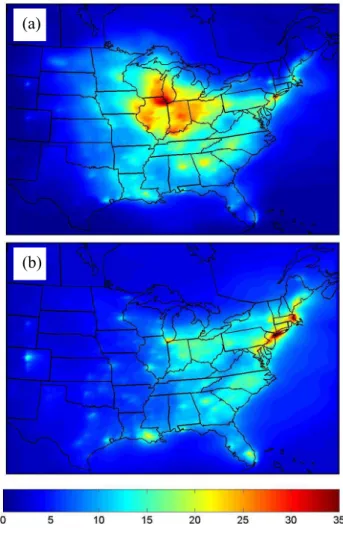
Fig. 1. Average PM2.5 concentrations (µg m−3)for the modeled
periods of (a) July 2001 and (b) January 2002.
O’Brien (1970) (approximately two-thirds of grid cell time steps in July and half of grid cell time steps in January). This corresponded to average changes in mixing height of approximately 150 m. The area of cloud cover and precipita-tion were changed by growing (or shrinking) existing cloudy or precipitating areas into randomly selected adjacent cells. Cloud cover and precipitation were changed independently of one another so that their effects could be separated. A list of model processes affected by these meteorological changes is also given in Table 1. Emissions of all pollutants, biogenic and anthropogenic, were kept constant in all tests.
The model used a fixed concentration of each PM2.5 species as boundary conditions. The fixed concentrations indicate an assumption that there is no change in the long range transport of pollution to the US. The elemental car-bon boundary condition was 0.1 µg m−3in both months. In January, the following concentrations were used for bound-ary conditions: OM, 0.5 µg m−3; sulfate, 0.7 µg m−3; ni-trate, 0.3 µg m−3; ammonium, 0.35 µg m−3. July simula-tions used a different set of boundary concentrasimula-tions: OM,
2.5
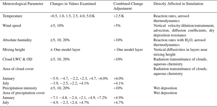
Table 1. Meteorological perturbations imposed in this study and adjustments imposed in combined-change simulation.
Meteorological Parameter Changes in Values Examined Combined-Change
Adjustment
Directly Affected in Simulation
Temperature +0.5, 1.0, 1.5, 2.5, 4.0, 5.0 K +2.5 K Reaction rates, aerosol
thermodynamics
Wind speed ±5, 10% +5% Vertical velocity/dilution/entrainment,
advection, diffusion coefficients, dry deposition resistance
Absolute humidity ±5, 10, 20% +10% Reaction rates with H2O, aerosol
thermodynamics
Mixing height ± One model layer + One model layer Vertical diffusivities in layers near
mixing height
Cloud LWC & OD ±5, 10, 20% +10% Radiation transmittance of clouds,
aqueous chemistry
Area of cloud cover Radiation transmittance of clouds,
aqueous chemistry
January −5.9, −4.7, −2.2, +2.3, +4.7, +6.0% +6.0%
July −3.9, −2.5, +2.2, +4.1% +4.1%
Precipitation intensity ±5, 10, 20% +10% Wet deposition
Area of precipitation cover Wet deposition
January −7.1 −4.8, −2.4, +2.1, +4.9, +7.2% +4.9% July −4.9, −2.3, +2.4, +4.7% +4.7% 0 1 2 3 4 5 6 7 8 A v e ra g e P M2 .5 c o n c e n tr a ti o n ( µ g m -3 ) January July PM2.5 NO3- SO42- NH4+ SOA POA
Fig. 2. Simulation-long land cell average concentrations (µg m−3)
of total PM2.5and PM2.5nitrate, sulfate, ammonium, secondary
or-ganic aerosol (SOA), and primary oror-ganic aerosol (POA) in January and July base case simulations.
0.8 µg m−3; sulfate, 0.9 µg m−3; nitrate, 0.1 µg m−3; ammo-nium, 0.37 µg m−3(Karydis et al., 2007). Boundary condi-tions of aerosol species were split equally among the six size bins that comprised PM2.5.
Simulation-averaged ground-level concentrations of total PM2.5 as well as PM2.5 ammonium, sulfate, nitrate, and organics are the species examined in this analysis. The base case predicted concentrations of total PM2.5 for both
months are shown in Fig. 1, and the land-cell average con-centrations for the species investigated for both months are shown in Fig. 2. Average ground-level concentrations of total PM2.5 were 5.8 µg m−3in January and 6.9 µg m−3 in July. In January, the highest simulation-average concentra-tion was 40 µg m−3 in the New York area, due largely to primary organics. In July, the highest average concentra-tions (up to 44 µg m−3)were in the Midwest, especially the Chicago area; this was largely due to high sulfate concen-trations. Nitrate concentrations were relatively high during January (Fig. 2), while sulfate concentrations were high dur-ing July. SOA concentrations were higher durdur-ing July, while POA concentrations changed little with season. SOA com-prised 54% of total OM in July, though its contribution was reduced to 17% in January.
3 Results and discussion
3.1 Temperature
The response of PM2.5 concentrations to temperature was largely the result of competing changes in sulfate and ni-trate concentrations with a smaller role played by organ-ics. In January, average PM2.5 concentrations over land grid cells decreased by 170 ng m−3K−1 (2.9% K−1), while average concentrations in July decreased by 16 ng m−3K−1 (0.23% K−1). In January, when nitrate concentrations were high, the response of total PM2.5 was stronger than in July, when nitrate concentrations were low. Total PM2.5
-250 -200 -150 -100 -50 0 50 100 ∆ PM 2 .5 s p e c ie s c o n c e n tr a ti o n ( n g m -3) +0.5 K +1.0 K +2.5 K +4.0 K +5.0 K NH4 + NO3 -SO4 2-SOA POA -250 -200 -150 -100 -50 0 50 100 ∆ PM 2 .5 s p e c ie s c o n c e n tr a ti o n ( n g m -3) +0.5 K +1.0 K +1.5 K +2.5 K +4.0 K +5.0 K NH4 + NO3 -SO4 2-SOA POA (a) January (b) July
Fig. 3. Average differences in simulation-averaged ground-level
PM2.5 species concentrations in (a) January and (b) July for
per-turbed temperature cases.
concentrations decreased by 2.9% K−1 in January and by 0.23% K−1 in July, resulting in an average reduction of 1.6% K−1.
In July, temperature increases led to increases in sulfate concentrations and simultaneous decreases in nitrate and organic concentrations. In January, however, average ni-trate and organic concentrations still decreased as tempera-ture was increased, but average sulfate concentrations were rather insensitive to temperature changes. Changes in am-monium were a consequence of the changes in nitrate and sulfate. These average changes are shown in Fig. 3. Aver-age PM2.5nitrate concentrations over land cells decreased by 120 ng m−3K−1(19% K−1)and 26 ng m−3K−1(17% K−1) in January and July respectively. This is mostly due to the volatilization of ammonium nitrate, which partitions to the gas phase at higher temperatures (Seinfeld and Pandis, 2006). Average PM2.5 sulfate concentrations over land cells in-creased by 1.6 ng m−3K−1(0.12% K−1)and 34 ng m−3K−1 (1.3% K−1)in January and July respectively. This link be-tween sulfate concentrations and temperature is due to the
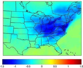
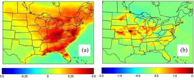
Fig. 4. Average changes in total PM2.5 (µg m−3) January for a
2.5 K temperature increase.
increased rate of oxidation of SO2 at higher temperature, caused by temperature-dependent rate constants and higher concentrations of oxidants. Average concentrations over land grid cells of total organic PM2.5decreased by 13 ng m−3K−1 (0.90% K−1) and 14 ng m−3K−1 (0.75% K−1) in January and July respectively. This is the net effect of increased gas-phase partitioning and faster gas-to-particle conversion at higher temperatures (Strader et al., 1999). In January, SOA accounted for 17% of organic mass over land cells and 42% of the response of organic PM2.5mass to a 2.5 K temperature increase; in July, SOA accounted for 54% of organic mass and 59% of the corresponding temperature response. The stronger effect of temperature on nitrate than on organics was also suggested by Aw and Kleeman (2003). Average nitrate concentrations decreased by 15% K−1 on average, organic concentrations decreased by 1.0% K−1, and sulfate concen-trations increased by 0.12% K−1in January and 4.2% K−1in July.
The sensitivities to temperature changes were nonuniform throughout the domain. In some places, the response of total PM2.5was dominated by decreases in nitrate, while in other places increases in sulfate were dominant (Figs. 4 and 5). In January, the response of total PM2.5 (Fig. 4) was very sim-ilar to that of PM2.5 nitrate. The response in January was rather homogeneous throughout the domain (Fig. 4). In July, the response of total PM2.5 (Fig. 5a) reflected the combined responses of nitrate (Fig. 5b) and sulfate (Fig. 5c). The in-creases in sulfate and dein-creases in nitrate offset each other to lead to a small response in average total PM2.5. The re-sponse of PM2.5concentrations in July was much more vari-able spatially than the response in January. Changes in or-ganics tended to be rather small (averaging −14 ng m−3K−1 with a maximum sensitivity of −100 ng m−3K−1in July), and changes in PM2.5ammonium appear to have been largely influenced by the changes in nitrate and sulfate.
2.5
(b)
(c)
(a)
Fig. 5. Average changes in (a) total PM2.5(µg m−3), (b) PM2.5nitrate, and (c) PM2.5sulfate in July for a 2.5 K temperature increase.
Table 2. Simulation-average sensitivities to meteorological perturbations in Pittsburgh in Atlanta.
January July Units
Pittsburgh Atlanta Pittsburgh Atlanta
Temperature −2.2 −2.1 0.26 −0.68 % K−1 Wind speed −0.83 −0.71 −0.73 −0.93 % %−1 Absolute humidity 0.12 0.15 0.06 0.22 % %−1 Mixing height −0.9 −1.1 −1.2 −1.5 % (100 m)−1 LWC and OD −0.02 −0.02 −0.002 −0.003 % %−1 Cloudy area −0.1a −0.04 −0.09 −0.2 % %−1 Precipitation rate −0.01 −0.01 −0.1 −0.2 % %−1 Precipitation area −0.001 −0.001 −0.1 −0.3 % %−1
aFor an increase in cloudy area. Smaller sensitivity for decrease in cloudy area (Sect. 3.6).
In January, simulation-averaged concentrations of total PM2.5 decreased by 300 ng m−3K−1 (−2.1% K−1) in At-lanta and 400 ng m−3K−1 (−2.2% K−1)in Pittsburgh (Ta-ble 2). In contrast, July concentrations of PM2.5 decreased by 150 ng m−3K−1(−0.68% K−1)in Atlanta and increased by 60 ng m−3K−1(+0.26% K−1)in Pittsburgh. The January
responses in both cities were dominated by decreases in ni-trate, while the July responses were the results of the com-bined responses of nitrate, sulfate, and organics. Western Ohio and the Great Lakes region, where nitrate concentra-tions were relatively high in both January and July, experi-enced the largest decreases with increased temperature due
to nitrate decreases, while the Ohio River Valley experienced the largest increases in July due to increases in sulfate. The response to a temperature increase in Chicago was dominated by increases in sulfate in July and decreases in nitrate in Jan-uary.
3.2 Wind speed
Wind speed changes affected all species that comprised PM2.5, with increases in wind speed generally leading to de-creases in PM2.5concentrations, and decreases in wind speed generally leading to increases in PM2.5. The simulation-long average PM2.5 concentration over land grid cells decreased with increasing wind speed by 30 ng m−3%−1(0.56% %−1) and 50 ng m−3%−1 (0.77% %−1) in January and July re-spectively. Changes in concentrations were greatest in the populated and polluted areas of the domain and smaller (or nearly zero) in more remote areas. The largest decrease in concentrations in January was in the New York area (270 ng m−3%−1or 0.68% %−1), while the largest concen-tration decrease in July was near Chicago (340 ng m−3%−1 or 0.77% %−1). Concentrations in both Atlanta and Pitts-burgh also decreased with increased wind speed (Table 2). These results are consistent with the observed association between high PM concentrations and stagnation (and, there-fore, low wind speed) (Triantafyllou et al., 2002).
The above changes in concentrations are largely due to changes in advection and dispersion with wind speed, with changes in dry deposition playing a relatively small role. Be-cause westerly winds are most common over the Eastern US, increased wind speeds carry additional PM out to the ocean. The resultant absolute changes in PM2.5 concentrations ap-pear to be minor in areas with low PM concentrations, but appreciable in more polluted areas. The relative sensitivities were roughly uniform, between −0.5 and −0.9% %−1, in-dicating an important impact of changes in wind speed on PM2.5concentrations.
3.3 Absolute humidity
Changes in absolute humidity had the largest effects on con-centrations of ammonium nitrate aerosol with concon-centrations increasing with increased absolute humidity (Fig. 6). This ef-fect was somewhat stronger during the summer, when water vapor, nitric acid, and ammonia concentrations are highest.
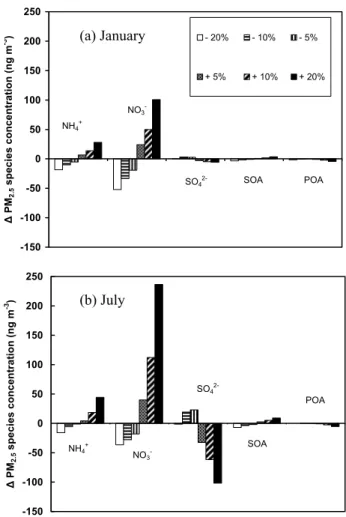
The simulation-long average PM2.5 concentration over land grid cells increased with water vapor concentra-tion by 14 ng m−3%−1 (0.24% %−1) and 20 ng m−3%−1 (0.29% %−1)in January and July respectively, while nitrate concentrations changed by 11 ng m−3%−1(1.7% %−1)and 23 ng m−3%−1(15% %−1)respectively. Changes in average concentrations for a 10% increase in water vapor are shown in Fig. 7. Increases in humidity shift the equilibrium of the ammonia-nitric acid system toward the aerosol phase, result-ing in higher concentrations of ammonium nitrate aerosol
-150 -100 -50 0 50 100 150 200 250 ∆ PM 2 .5 s p e c ie s c o n c e n tr a ti o n (n g m -3 ) - 20% - 10% - 5% + 5% + 10% + 20% NH4 + NO3 -SO4 2- SOA POA -150 -100 -50 0 50 100 150 200 250 ∆ PM 2 .5 s p e c ie s c o n c e n tr a ti o n ( n g m -3 ) NH4 + NO3 -SO4 2-SOA POA (a) January (b) July
Fig. 6. Changes in simulation-long ground-level average PM2.5
species concentrations in (a) January and (b) July perturbed abso-lute humidity simulations.
(Seinfeld and Pandis, 2006). Changes in sulfate aerosol were relatively small in summer (roughly half the changes in aver-age nitrate) and practically negligible in winter, and changes in organics were negligible in both seasons. Ammonium con-centrations appear to have been influenced by the changes in nitrate and, to a lesser extent, sulfate. The spatial distribu-tion of changes of average total PM2.5strongly resembled the changes in PM2.5nitrate. The areas of increased total PM2.5 (Figs. 7a and b) corresponded to the areas of increased PM2.5 nitrate.
Changes in nitrate accounted for most of these total changes in Atlanta in Pittsburgh (Table 2); other species changed little compared to nitrate aerosol. These changes and the changes over the entire domain indicate that the ef-fects of absolute humidity on PM2.5 concentrations are po-tentially important, especially the effect on PM2.5nitrate.
2.5
(a)
(b)
Fig. 7. Average changes in total PM2.5(µg m−3)in (a) January and (b) July for a 10% increase in absolute humidity.
(b)
(a)
Fig. 8. Average changes in PM2.5concentrations (µg m−3)due to
a one-layer decrease (approximately 150 m) in mixing height in (a) January and (b) July.
3.4 Mixing height
Changes in mixing height had effects on all aerosol species. As expected, increases in mixing height led to decreases in PM2.5 concentrations. Species were affected roughly in proportion to their relative concentrations, indicating that the mixing height effect is a simple dilution effect that does not induce major chemical feedbacks. In January and July, the average land cell PM2.5concentration decreased by 73 ng m−3 (100 m)−1 (−1.3% (100 m)−1) and 210 ng m−3 (100 m)−1(−3.0% (100 m)−1)respectively. The difference between seasons is mainly due to lower mixing heights in July during the period modeled. The simulation-average base-case mixing height was 620 m in January and 420 m in July, the lower mixing height in July being a consequence of the periods selected. Generally, mixing heights tend to be lower in winter than in summer, meaning that changes in mixing height would affect winter concentrations more strongly than summer concentrations.
The simulation-averaged changes in PM2.5 due to an in-crease in mixing height are shown in Fig. 8. The effect of mixing height on PM2.5concentrations in Atlanta and Pitts-burgh was significant in both seasons (Table 2). The effect of mixing height on PM2.5concentrations, therefore, appears to be rather important, especially in polluted areas.
3.5 Cloud liquid water content and optical depth
Neither total PM2.5 concentrations nor any aerosol species showed a strong sensitivity to changes in cloud LWC and OD (at constant cloudy area). Base case cloud cover and rain are shown in Fig. 9. In January and July, the land-cell aver-age PM2.5concentration decreased with increased LWC and OD by 0.9 ng m−3%−1 and 1.7 ng m−3%−1 (−0.02% %−1 for both seasons) respectively. The average sensitivities of all species during both months were less than 1 ng m−3%−1.
(a)
(b)
(c)
(d)
Fig. 9. Column- and simulation-averaged base case (a) January cloud water content (g m−3), (b) January precipitation water content (g m−3),
(c) July cloud water content (g m−3), and (d) July precipitation water content (g m−3).
Pandis and Seinfeld (1989) calculated a relatively small change in total aqueous sulfate for an increase in LWC in-side a single cloud. The net effect of these small changes in sulfate chemistry during cloudy periods several hundred meters aloft is a minor change in average PM2.5 at ground level.
Average concentrations of total PM2.5in both Atlanta and Pittsburgh changed rather little with cloud LWC and OD (Ta-ble 2). The largest sensitivity of total PM2.5 concentrations in July was −70 ng m−3%−1(−0.28% %−1)near St. Louis, and the largest sensitivity in January was −50 ng m−3%−1 (−0.13% %−1)near Boston. Even these extreme values are rather small, indicating that the effects of cloud LWC and OD (at fixed cloudy area) on PM2.5concentrations are of mi-nor importance. The location-specific responses, especially for the cloud and rain parameters, are largely a consequence of the period modeled and the relatively short duration of the study. These differences between location-specific responses
do not necessarily mean that one location is inherently more sensitive to changes in clouds and precipitation, but they do give an estimate of the range of sensitivities.
3.6 Cloudy area
The influence of cloudy area on PM2.5concentrations varied by season and location, and all simulation-average changes, both domain-wide and in specific locations, were rather small. The mechanisms by which changes in cloudy area affect PM2.5 concentrations is essentially the same as the mechanism by which cloud LWC and OD affect concen-trations. In both January and July, increases in cloudy area led to decreases in simulation-averaged PM2.5 over land grid cells. This average decrease was 2 ng m−3%−1 (−0.03% %−1)in January and 14 ng m−3%−1(−0.2% %−1)
in July. The differences in simulation-average ground-level concentrations of major PM2.5 species due to changes
2.5
(b)
(a)
Fig. 10. Changes in simulation-long ground-level average
concen-tration of major PM2.5 species with changing cloudy area in (a)
January and (b) July.
in cloudy area are shown in Fig. 10. In January, aver-age nitrate (−2 ng m−3%−1 or −0.3% %−1) and organics (−1 ng m−3%−1or −0.1% %−1)decreased with increased cloud cover, while average sulfate increased (2 ng m−3%−1 or 0.1% %−1). In July, all species decreased with increased cloud cover, with both sulfate and organics decreasing by 5 ng m−3%−1(−0.2% %−1and −0.3% %−1, respectively). The difference between seasons in the sulfate response is due to the greater relative importance of aqueous sulfate produc-tion in January than in July.
The responses in Pittsburgh and Atlanta PM2.5 concen-trations to changes in cloud cover were mixed and rather small (Table 2). In January, the Pittsburgh PM2.5 concen-tration increased by 0.3 ng m−3%−1(−0.002% %−1)for the 5.9% cloud cover decrease, and decreased by 20 ng m−3%−1 (−0.1% %−1)for a 6% cloud cover increase. January PM2.5 concentrations in Atlanta, however, were affected little by either a 5.9% cloud cover decrease (−7 ng m−3%−1 or
−0.05% %−1)or a 6.0% cloud cover increase (5 ng m−3%−1
or −0.03% %−1). In both cities in January, average ni-trate and ammonium decreased as cloud cover was increased. PM2.5concentration in July decreased with increased cloud cover by 20 ng m−3%−1 (−0.09% %−1) in Pittsburgh and 50 ng m−3%−1(−0.2% %−1)in Atlanta. In both cities, the July sensitivity to cloud cover changes was dominated by changes in sulfate, which decreased as cloud cover was in-creased. The changes in PM2.5 resulting from cloud cover changes were rather small, and it appears that they are of secondary importance to PM2.5concentrations.
3.7 Precipitation rate
Changes in the rate of precipitation affected PM2.5 concen-trations more strongly in July than in January. Changes in simulation-average PM2.5 for a 10% decrease in precipita-tion rate in July are shown in Fig. 11. Sensitivities in much of the Midwest and Southeast were between 0.3 and 0.5% %−1. Sensitivities larger than 0.3% %−1covered a large portion of the domain. The changes in PM2.5resulted even in areas with little or no base-case precipitation (Fig. 9d), such as northern Indiana (Fig. 11b), indicating that changes in precipitation in upwind areas affected PM2.5concentrations in downwind areas.
In both Pittsburgh and Atlanta, the sensitivity of total PM2.5 to changes in precipitation rate was over an order of magnitude larger in July than in January (Table 2). This is due in part to the differences in precipitation between the two months (Fig. 9) causing a percentage adjustment in pre-cipitation to represent a different amount of rainfall in each month. There is also an effect of the differences in the type of precipitation between the two seasons. In the Eastern USA, large-scale precipitation tends to dominate in winter, while convective precipitation is important in summer. Since con-vective storms tend to be short-lived, changes in precipita-tion rate help them more fully wash out aerosols. The overall wet removal by large-scale systems, which generally have a longer lifetime, is less sensitive to the precipitation rate since there is more time to fully wash out aerosols from the air. Areas with heavy base-case precipitation, such as the south-eastern section of the domain, southern Missouri, Kansas, and the Dakotas (Fig. 9d), had small sensitivities to precipi-tation changes (Fig. 11). The areas with the largest sensitiv-ities (Fig. 11) were the areas with smaller amounts of base-case precipitation, such as the Great Lakes region and West Virginia (Fig. 9d).
The sensitivities of PM2.5 concentrations to precipitation rate (with fixed area of precipitation) were rather large over much of the domain. Overall land-average sensitivities were comparable to those of other meteorological parameters:
−0.02% %−1in January and −0.2% %−1in July. The small
sensitivity in January is partly a consequence of the lack of modeled precipitation in areas such as the Great Lakes region and New England (Fig. 9b) that tend to receive substantial precipitation in January. Precipitation in July compared more
(b)
(a)
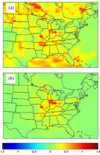
Fig. 11. Percent changes in simulation-average PM2.5
concentra-tions divided by percent decrease in precipitation rate (% %−1)(a),
and changes in simulation-average PM2.5concentration (µg m−3)
(b), both calculated for a 10% reduction in precipitation rate in July.
favorably to measured precipitation. Additionally, snow and ice were assumed not to remove pollutants in the model. These results indicate that there is a moderate effect of pre-cipitation rate (with fixed area of prepre-cipitation) on PM2.5 concentrations, with the strongest relative effect (in terms of percent change in PM2.5)in areas receiving light to moderate rainfall and in their downwind areas.
3.8 Precipitation area
The effects of changes in area of precipitation were again more pronounced in July than in January. The area of precip-itation was defined as the average fraction of grid cells over which precipitation at any hour during the simulation. The simulation-average changes due to a 4.9% decrease in precip-itating area in July are shown in Fig. 12. These changes were substantial over a large portion of the domain. Simulation-average sensitivities more negative than −0.45% %−1
cov-(b)
(a)
Fig. 12. Percent changes in simulation-average PM2.5
concentra-tions divided by percent decrease in precipitating area (% %−1)(a),
and changes in simulation-average PM2.5 concentration (µg m−3)
(b), calculated for a 4.9% decrease in area of precipitation in July.
ered much of the domain in July (Fig. 12), though in January the differences in nearly all areas were between −0.3% %−1 and zero. The average land-cell sensitivity of total PM2.5 to the change in precipitating area in July was −15 ng m−3%−1 (−0.2% %−1)while the average sensitivity in January was a factor of 50 smaller.
Pittsburgh and Atlanta were both more greatly affected by changes in precipitating area in July than in Jan-uary (Table 2). In both cities in January, sensitivities were on the order of 0.1 ng m−3%−1 (0.001% %−1). In July, concentrations in Atlanta decreased by 60 ng m−3%−1 (−0.3% %−1), while concentrations in Pittsburgh decreased by 20 ng m−3%−1 (−0.1% %−1). These two cities, how-ever, were affected less by changes in precipitation than much of the Midwest due to the location of precipitation in these cases (Fig. 9). Near St. Louis, absolute values of the sensitivities were near 350 ng m−3%−1 (approximately
−1.5% %−1). The impact of the area of precipitation on
2.5 -1 0 1 2 3 4 5 -1 0 1 2 3 4 5
Reduction due to combined met changes (µg m-3)
Su m m e d i n d iv id u a l c h a n g e s (µ g m -3) -1 0 1 2 3 4 5 6 7 -1 0 1 2 3 4 5 6 7
Reduction due to combined met changes (µg m-3)
S u m m e d i n d iv id u a l c h a n g e s (µ g m -3) (a) (b)
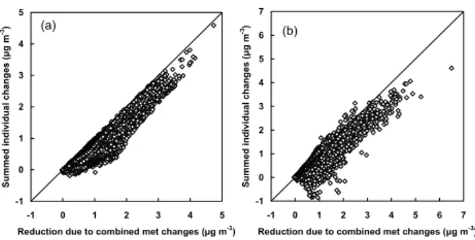
Fig. 13. Sum of changes in PM2.5concentrations from separate
me-teorological perturbations versus changes due to combined meteo-rological perturbations in (a) January and (b) July. Each data point represents a simulation-average concentration in one grid cell. All values have been multiplied by −1 for easier viewing. Lines are 1:1 lines.
important one, due to the large response in a rather small area, rather than a large mean response.
4 Additivity of effects
Two additional simulations were run in which perturbations in all eight meteorological parameters were imposed in both months. These perturbations are listed in Table 1. The result-ing changes in average concentrations were compared to the sum of the changes that resulted when the perturbations were imposed individually. For simulation-long land-cell averages in July of total PM2.5, ammonium, sulfate, and organics, the signs of the two predictions agreed. Both methods yielded predicted changes in simulation- and land-cell-average ni-trate close to zero. The predicted changes in simulation- and land-cell-average sulfate were within 20% (or 0.03 µg m−3) of one another, and predicted changes in organics differed by only 0.01 µg m−3. Predicted changes in total PM2.5differed by 22%, or 0.15 µg m−3. In January, both methods predicted the same signs for changes in total PM2.5, ammonium, sul-fate, nitrate, and organics. Predicted changes in total aver-age PM2.5in January differed by 0.28 µg m−3, or 32%. Pre-dicted changes in average organics and nitrate were within 10% of each other, while there was a factor of 6 difference (0.21 µg m−3)in predicted sulfate changes in January
A plot of the sum of individual changes in PM2.5 con-centrations versus the changes resulting from the combined-change simulation are shown in Fig. 13. The two combined-changes were rather well correlated (R=0.95 in January and 0.94 in July), and the slope of the linear fit of the summed individ-ual changes versus the combined changes was 0.73 in Jan-uary and 0.77 in July. The summed individual changes were on average 27% smaller than the predicted changes from the combined-change simulation in January and 23% smaller in July. This is a reasonable agreement between the two meth-ods, at least in this case.
5 Relative importance of meteorological parameters
The relative importance of the various meteorological param-eters was estimated by taking into account the average sen-sitivities of total PM2.5 to the meteorological perturbations, the spatial variability of sensitivities, and potential future changes in the meteorological parameters. The mean sen-sitivities were multiplied by climate-model-predicted meteo-rological changes to yield estimates of changes in total PM2.5 concentrations due to each parameter. The mean sensitivities were calculated using the highest- and lowest-perturbation simulations for each variable, over which the sensitivities were roughly linear. These changes are summarized in Ta-ble 3. The work predicting these meteorological changes is summarized in Dawson et al. (2007).
Sensitivities of PM2.5 to changes in absolute humidity were calculated using only positive humidity changes, while sensitivities to cloudy area were calculated using only neg-ative cloudy area changes (due to the nonlinear overall re-sponses to these parameters and given consensus regarding the sign of their future changes). Expected meteorological changes are average changes corresponding to doubled CO2 concentrations for temperature and absolute humidity, 2050 projections for wind speed and precipitating area, and a 4 K sea surface temperature (SST) perturbation for cloudy area. The projections for 2050 are more modest than the doubled CO2 and 4 K SST increase, so changes in wind speed and precipitating area may be underrepresented. The precipitat-ing area change was inferred from predicted changes in total precipitation over the Eastern USA (Leung and Gustafson, 2005). Changes in mixing height, cloud LWC and OD, and precipitation intensity were chosen so that somewhat liberal estimates of the total PM2.5 sensitivity could be calculated and compared to the sensitivities to other parameters. The mean and 1st and 99th percentile values for sensitivities of total PM2.5 concentrations were included so that the spatial variability of sensitivities could be taken into account. Tem-perature, absolute humidity, wind speed, and mixing height led to the largest PM2.5 changes in January (with mean pre-dicted responses on the order of hundreds of ng m−3), while in July, absolute humidity, wind speed, mixing height, pre-cipitation intensity, and precipitating area all had potentially major effects on PM2.5 (Table 3). Temperature had little im-pact on mean July concentrations due to the competing ef-fects on nitrate, sulfate, and organics; in January, the volatil-ity of nitrate aerosol became dominant, causing larger de-creases in PM2.5with increasing temperature. The range for the mean predicted effect of temperature on PM2.5 concen-trations was −24 to −71 ng m−3in July; in January the range was −260 to −770 ng m−3. Neither cloud nor precipitation changes had a major impact on mean January PM2.5 (with mean predicted changes less than or equal to 20 ng m−3), though variability in the response to precipitation intensity indicates that it may be a somewhat important variable (with predicted responses up to 150 ng m−3). In July, temperature,
Table 3. Summary of expected meteorological changes and their effects on PM2.5concentrations in January and July. (Major sensitivities in
bold).
Meteorological Parameter Predicted Change Sensitivity Predicted Effect (ng m−3) Sensitivity Mean Predicted Effect (ng m−3)
of Parameter Mean (1%, 99%) Mean (1%, 99%) (1%, 99%) Mean (1%, 99%)
Temperature +1.5 to +4.5 Ka −171 ng m−3K−1 (−463, −6.83) −770 to −260 (−2100 to −10) −16 ng m−3K−1 (−238, 101) −71 to −24 (−1100 to 450) Absolute humidity +7 to +21%b 14 ng m−3%−1 (0.078, 36.3) 99 to 300 (0.55 to 760) 20 ng m−3%−1 (−28.2, 133) 140 to 410 (−590 to 2800) Wind speed −1.4 to −4.5%c −33 ng m−3%−1 (−142, 12.3) 45 to 150 (−55 to 640) −53 ng m−3%−1 (−215, 3.88) 75 to 240 (−17 to 970)
Mixing height −1 layer to +1 layerd
(−150 m to +150 m) −73 ng m−3(100 m)−1 (−629, 58.6) −110 to 110 (−630 to 630) −210 ng m−3(100 m)−1 (−1290, 3.67) −310 to 310 (−1300 to 1300) Cloud LWC and OD −15 to +15%d −0.9 ng m−3%−1 (−5.28, 0.185) −14 to 14 (−80 to 80) −1.8 ng m−3%−1 (−14.1, 2.28) −26 to 26 (−210 to 210) Cloudy area −4.4 to −0.2%e −1.7 ng m−3%−1 (−17.5, 20.8) 0.34 to 7.6 (−92 to 77) −14 ng m−3%−1 (−99.4, 10.0) 2.9 to 64 (−44 to 440) Precipitation rate −20 to +20%d −1.0 ng m−3%−1 (−7.51, 0.082) −20 to 20 (−150 to 150) −17 ng m−3%−1 (−68.2, −0.037) −330 to 330 (−1400 to 1400) Precipitating area −10 to +10%f −0.4 ng m−3%−1 (−4.13, 0.381) −3.7 to 3.7 (−41 to 41) −15 ng m−3%−1 (−97.5, −0.0016) −150 to 150 (−980 to 980) aIPCC, 2001
bBased on IPCC temperature projections and constant 80% RH.
cBreslow and Sailor, 2002
dEspecially speculative; included to enable intercomparison among all parameters.
eCess et al., 1990
fIPCC Data Distribution Centre: http://ipcc-ddc.cru.uea.ac.uk/sres/scatter plots/scatterplots region.html
cloudy area, and cloud LWC and OD had smaller but po-tentially important effects if variability is taken into account (with responses up to several hundred ng m−3).
6 Conclusions
The strongest of the effects of changes in meteorology on PM2.5 concentrations were the effects of temperature, wind speed, absolute humidity, mixing height, and precipitation. Wind speed, mixing height, and precipitation affected all PM species. Temperature increased average sulfate tions and decreased average nitrate and organics concentra-tions. The main effect of increased absolute humidity was increased nitrate aerosol. These effects could lead to appre-ciable changes in PM2.5concentrations under a changed fu-ture climate.
The response of PM2.5 concentrations to changes in me-teorology was the net effect of the changes in individual aerosol species. The qualitative behavior of the key pro-cesses responsible for these sensitivities should not generally be very sensitive to choice of modeled time periods, even though the calculated sensitivities are dependent on the time period and base case meteorology. PM2.5 concentrations had a rather small response to temperature changes in sum-mer (−16 ng m−3K−1on average), due largely to increases in sulfate canceling decreases in nitrate and organics, while PM2.5 concentrations in winter decreased more strongly (−170 ng m−3K−1on average) because of reductions in ni-trate and organics. PM2.5 concentrations increased with
in-creased absolute humidity in both winter (14 ng m−3%−1)
and summer (20 ng m−3%−1), driven largely by increases in nitrate concentrations. Mixing height changes led to mixing and dilution effects, with PM2.5concentrations generally de-creasing as mixing height was increased. The mean effect of mixing height changes was nearly 3 times larger in July than in January, due to lower average mixing heights during the simulated July period and somewhat lower concentrations in January. Increases in wind speed led to changes in advection and transport resulting in decreases in PM2.5concentrations of 33 ng m−3%−1in January and 53 ng m−3%−1in July.
Cloud LWC and OD and cloudy area led to small changes in PM2.5 on average, but there were some areas with appre-ciable responses. Nitrate and organics generally decreased with increased cloud cover in both seasons; the same was true for sulfate in July, but not in January. As expected, PM2.5concentrations decreased with increased precipitation rate and precipitating area, though the sensitivities to changes in these precipitation parameters were over a factor of 10 larger in July than in January. The differences between sea-sons can be due to the differences in the dominant types of precipitation between the two seasons (large-scale in win-ter versus convective in summer), the rather small amount of precipitation in the modeled January period (Fig. 9), and the lack of scavenging by snow in the model. The largest mean expected changes for the imposed precipitation changes were between 0.1 to 0.8 µg m−3(Table 3), though the spatial vari-ability in responses could mean precipitation-driven changes in PM2.5of up to approximately 3 µg m−3(Table 3).
2.5
The potential for changes in average concentrations of sev-eral µg m−3indicates that changes in meteorology can have important impacts on PM2.5 concentrations. The changes in concentrations caused by changes in meteorology should, therefore, be taken into account in long-term air quality plan-ning.
Acknowledgements. This work was supported by US
Environ-mental Protection Agency STAR Grant # RD-83096101-0 and a National Science Foundation Graduate Research Fellowship. Edited by: A. Nenes
References
Aw, J. and Kleeman, M. J.: Evaluating the first-order effect of in-traannual temperature variability on urban air pollution, J. Geo-phys. Res., 108, 4365, doi: 10.1029/2002JD002688, 2003. Baertsch-Ritter, N., Keller, J., Dommen, J., and Prevot, A. S. H.:
Effects of various meteorological conditions and spatial emission
resolutions on the ozone concentration and ROG/NOxlimitation
in the Milan area (I), Atmos. Chem. Phys., 4, 423–438, 2004, http://www.atmos-chem-phys.net/4/423/2004/..
Bernard, S. M., Samet, J. M., Grambsch, A., Ebi, K. L., and Romieu, I.: The potential impact of climate variability and change on air pollution-related health effects in the United States, Environ. Health Perspect., 109, Suplm. 2, 199–209, 2001. Bogardi, I. and Matyasovszky, I.: Estimating daily wind speed
un-der climate change, Sol. Energy, 57, 239–248, 1996.
Brasseur, G. P., Kiehl, J. T., M¨uller, J.-F., Schneider, T., Granier, C., Tie, X., and Hauglustaine, D.: Past and future changes in global tropospheric ozone: Impact on radiative forcing, Geophys. Res. Lett., 25, 3807–3810, 1998.
Brasseur, G. P., Schultz, M., Granier, C., Saunois, M., Diehl, T., Botzet, M., Roeckner, E., and Walters, S.: Impact of climate change on the future chemical composition of the global tropo-sphere, J. Climate, 19, 3932–3951, 2006.
Breslow, P. B. and Sailor, D.J.: Vulnerability of wind power re-sources to climate change in the continental United States, Re-new. Energ., 27, 585–598, 2002.
Capaldo, K. P., Pilinis, C., and Pandis, S. N.: A computationally efficient hybrid approach for dynamic gas/aerosol transfer in air quality models, Atmos. Environ., 34, 3617–3627, 2000. Cess, R. D., Potter, G. L., Blanchet, J. P., Boer, G. J., DelGengio,
A. D., D´equ´e, M., Dymnikov, V., Galin, V., Gates, W. L., Ghan, S. J., Kiehl, J. T., Lacis, A. A., LeTreut, H., Li, Z.-X., Liang, X.-Z., McAvaney, B. J., Meleshko, V. P., Mitchell, J. F. B., Mor-crette, J.-J., Randall, D. A., Rikus, L., Roeckner, E., Royer, J. F., Schlese, U., Sheinin, D. A., Slingo, A., Sokolov, A. P., Taylor, K. E., Washington, W. M., Wetherald, R. T., Yagai, I., and Zhang, M.-H.: Intercomparison and interpretation of climate feedback processes in 19 atmospheric general circulation models, J. Geo-phys. Res., 95, 16 601–16 615, 1990.
Chang, J. S., Brost, R. A., Isaksen, I. S. A., Madronich, S., Middle-ton, P., Stockwell, W. R., and Walcek, C. J.: A three-dimensional Eulerian acid deposition model: Physical concepts and formula-tion, J. Geophys. Res., 92, 14 681–14 700, 1987.
Dawson, J. P., Adams, P. J., and Pandis, S. N.: Sensitivity of ozone to summertime climate in the Eastern US: A modeling case study, Atmos. Environ., 41, 1494–1511, 2007.
Elminir, H. K.: Dependence of urban air pollutants on meteorology, Sci. Total Environ., 350, 225–237, 2005.
Environ International Corporation (Environ): User’s guide: Com-prehensive air quality model with extensions (CAMx), Ver-sion 4.02, Environ International Corporation, Novato, California, 2004.
Fahey, K. M. and Pandis, S. N.: Optimizing model performance: variable size resolution in cloud chemistry modeling, Atmos. En-viron., 35, 4471–4478, 2001.
Gaydos, T. M., Pinder, R. W., Koo, B., Fahey, K. M., Yarwood, G., and Pandis, S. N.: Development and application of a three-dimensional aerosol chemical transport model, PMCAMx, At-mos. Environ., 41, 2594–2611, 2007.
Gery, M. W., Whitten, G. Z., Killus, J. P., and Dodge, M. C.: A photochemical kinetics mechanism for urban and regional scale computer modeling, J. Geophys. Res., 94, 925–956, 1989. Godish, T.: Air quality, Lewis Publishers, Boca Raton, Florida,
2004.
Held, I. M. and Soden, B. J.: Water vapor feedback and global warming, Annu. Rev. Energ. Env., 25, 441–475, 2000.
Hogrefe, C., Lynn, B., Civerolo, K., Ku, J.-Y., Rosenthal, J., Rosen-zweig, C., Goldberg, R., Gaffin, S., Knowlton, K., and Kin-ney, P. L.: Simulating changes in regional air pollution over the eastern United States due to changes in global and re-gional climate and emissions, J. Geophys. Res., 109, D22301, doi:10.1029/2004JD004690, 2004.
Intergovernmental Panel on Climate Change (IPCC): Climate change 2001: The scientific basis, Cambridge University Press, Cambridge, 2001.
Johnson, C. E., Stevenson, D. S., Collins, W. J., and Derwent, R. G.: Role of climate feedback on methane and ozone studied with a coupled Ocean-Atmosphere-Chemistry model, Geophys. Res. Lett., 28, 1723–1726, 2001.
Kappos, A. D., Bruckmann, P., Eikmann, T., Englert, N., Heinrich, U., H¨oppe, P., Koch, E., Krause, G. H. M., Kreyling, W. G., Rauchfuss, K., Rombout, P., Schulz-Klemp, V., Thiel, W. R., and Wichmann, H.-E.: Health effects of particles in ambient air, Int. J. Hyg. Environ. Health, 207, 399–407, 2004.
Karydis, V., Tsimpidi, A., and Pandis, S. N.: Evaluation of a three-dimensional chemical transport model (PMCAMx) in the East-ern United States for all four seasons, J. Geophys. Res., 112, D14211, doi:10.1029/2006JD007890, 2007.
Koch, D., Park, J., and DelGenio, A.: Clouds and sulfate are anti-correlated: A new diagnostic for global sulfur models, J. Geo-phys. Res., 108, 4781, doi:10.1029/2003JD003621, 2003. Koo, B., Gaydos, T. M., and Pandis, S. N.: Evaluation of the
equilibrium, dynamic, and hybrid aerosol modeling approaches, Aerosol Sci. Technol., 37, 53–64, 2003.
LADCO, Lake Michigan Air Directors Consortium: Base E
modeling inventory. Report prepared by Lake Michigan Air Directors Consortium, http://www.ladco.org/tech/emis/BaseE/ baseEreport.pdf, 2003.
Leung, L. R. and Gustafson, Jr., W. I.: Potential regional climate change and implications to U.S. air quality, Geophys. Res. Lett., 32, L16711, doi:10.1029/2005GL022911, 2005.
in global predictions of future tropospheric ozone and aerosols, J. Geophys. Res., 111, D12304, doi:10.1029/2005JD006852, 2006. Mickley, L. J., Jacob, D. J., Field, B. D., and Rind, D.: Effects of future climate change on regional air pollution episodes in the United States, Geophys. Res. Lett., 31, L24103, doi:10.1029/2004GL021216, 2004.
Murazaki, K. and Hess, P.: How does climate change contribute to surface ozone change over the United States?, J. Geophys. Res., 111, D05301, doi:10.1029/2005JD005873, 2006.
Norris, J. R.: Multidecadal changes in near-global cloud cover and estimated cloud cover radiative forcing, J. Geophys. Res., 110, D08206, doi:10.1029/2004JD005600, 2005.
Pandis, S. N. and Seinfeld, J. H.: Sensitivity analysis of a chemical mechanism for aqueous-phase atmospheric chemistry, J. Geo-phys. Res., 94, 1105–1126, 1989.
Racherla, P. N. and Adams, P. J.: Sensitivity of global
tropospheric ozone and fine particulate matter concentra-tions to climate change, J. Geophys. Res., 111, D24103, doi:10.1029/2005JD006939, 2007.
R¨ais¨anen, J.: Impact of increasing CO2on monthly-to-annual
pre-cipitation extremes: analysis of the CMIP2 experiments, Clim. Dynam., 24, 309–323, 2005.
Schwartz, J., Dockery, D. W., and Neas, L. M.: Is daily mortality associated specifically with fine particles?, J. Air Waste Manage. Assoc., 46, 927–939, 1996.
Seinfeld, J. H. and Pandis, S. N.: Atmospheric chemistry and physics: From air pollution to climate change, Third edition, John Wiley, New York, 2006.
Sheehan, P. E. and Bowman, F. M.: Estimated effects of tempera-ture on secondary organic aerosol concentrations, Environ. Sci. Technol., 35, 2129–2135, 2001.
Strader, R., Lurmann, F., and Pandis, S. N.: Evaluation of secondary organic aerosol formation in winter, Atmos. Environ., 33, 4849– 4863, 1999.
Steiner, A. L., Tonse, S., Cohen, R. C., Goldstein, A. H., and Harley, R. A.: Influence of future climate and emissions on re-gional air quality in California, J. Geophys. Res., 111, D18303, doi:10.1029/2005JD006935, 2006.
Sweet, C. W. and Gatz, D. F.: Summary and analysis of
avail-able PM2.5measurements in Illinois, Atmos. Environ., 32, 1129–
1133, 1998.
Triantafyllou, A. G., Kiros, E. S., and Evagelopoulos, V. G.: Res-pirable particulate matter at an urban and nearby industrial loca-tion: Concentrations and variability and synoptic weather condi-tions during high pollution episodes, J. Air Waste Manage. As-soc., 52, 287–296, 2002.
Unger, N., Shindell, D. T., Koch, D. M., Amann, M., Cofala, J., and Streets, D. G.: Influences of man-made emissions and climate changes on tropospheric ozone, methane, and sulfate at 2030 from a broad range of possible futures, J. Geophys. Res., 111, D12313, doi:10.1029/2005JD006518, 2006.
Wilkinson, J. and Janssen, M.: BIOME3. Prepared for
the National Emissions Inventory Workshop, Denver, CO, 1–3 May 2001, http://www.epa.gov/ttn/chief/conference/ei10/ modeling/wilkinson.pdf, 2001.
Wise, E. K. and Comrie, A. C.: Meteorologically adjusted urban air quality trends in the Southwestern United States, Atmos. Envi-ron., 39, 2969–2980, 2005.