HAL Id: hal-00296391
https://hal.archives-ouvertes.fr/hal-00296391
Submitted on 7 Dec 2007
HAL is a multi-disciplinary open access
archive for the deposit and dissemination of
sci-entific research documents, whether they are
pub-lished or not. The documents may come from
teaching and research institutions in France or
abroad, or from public or private research centers.
L’archive ouverte pluridisciplinaire HAL, est
destinée au dépôt et à la diffusion de documents
scientifiques de niveau recherche, publiés ou non,
émanant des établissements d’enseignement et de
recherche français ou étrangers, des laboratoires
publics ou privés.
estimates of NOx lifetimes and impact of the complex
Alpine topography on the retrieval
D. Schaub, D. Brunner, K. F. Boersma, J. Keller, D. Folini, B. Buchmann, H.
Berresheim, J. Staehelin
To cite this version:
D. Schaub, D. Brunner, K. F. Boersma, J. Keller, D. Folini, et al.. SCIAMACHY tropospheric NO2
over Switzerland: estimates of NOx lifetimes and impact of the complex Alpine topography on the
retrieval. Atmospheric Chemistry and Physics, European Geosciences Union, 2007, 7 (23),
pp.5971-5987. �hal-00296391�
www.atmos-chem-phys.net/7/5971/2007/ © Author(s) 2007. This work is licensed under a Creative Commons License.
Chemistry
and Physics
SCIAMACHY tropospheric NO
2
over Switzerland: estimates of
NO
x
lifetimes and impact of the complex Alpine topography on the
retrieval
D. Schaub1, D. Brunner1, K. F. Boersma2, J. Keller3, D. Folini1, B. Buchmann1, H. Berresheim4,*, and J. Staehelin5 1Empa, Swiss Federal Laboratories for Materials Testing and Research, Ueberlandstrasse 129, 8600 Duebendorf, Switzerland 2School of Engineering and Applied Sciences, Harvard University, Cambridge, Massachusetts, USA
3Paul Scherrer Institute (PSI), 5232 Villigen PSI, Switzerland
4German National Meteorological Service, DWD/MOHp, 82383 Hohenpeissenberg, Germany 5Swiss Federal Institute of Technology (ETH), Universit¨atstrasse 16, 8092 Zurich, Switzerland
*now at: National University of Ireland Galway, Department of Physics, University Road, Galway, Ireland
Received: 23 November 2006 – Published in Atmos. Chem. Phys. Discuss.: 12 January 2007 Revised: 9 November 2007 – Accepted: 21 November 2007 – Published: 7 December 2007
Abstract. This study evaluates NO2 vertical tropospheric
column densities (VTCs) retrieved from measurements of the Scanning Imaging Absorption Spectrometer for Atmospheric Chartography (SCIAMACHY) above Switzerland and the Alpine region. The close correlation between pixel averaged NOx emission rates from a spatially and temporally highly
resolved inventory and the NO2 VTCs under anticyclonic
meteorological conditions demonstrates the general ability of SCIAMACHY to detect sources of NOxpollution in
Switzer-land. This correlation is further used to infer seasonal mean NOxlifetimes carefully taking into account the influence of
the strong diurnal cycle in NOxemissions on these estimates.
Lifetimes are estimated to 3.6 (±0.8) hours in summer and 13.1 (±3.8) hours in winter, the winter value being some-what lower than previous estimates. A comparison between the 2003-2005 mean NO2 VTC distribution over
Switzer-land and the corresponding 1996–2003 mean from the Global Ozone Monitoring Experiment (GOME) illustrates the much better capability of SCIAMACHY to resolve regional scale pollution features. However, the comparison of seasonal av-erages over the Swiss Plateau with GOME and ground based in situ observations indicates that SCIAMACHY exhibits a too weak seasonal cycle with comparatively high values in summer and low values in winter. A problem likely con-tributing to the reduced values in winter (not reported in ear-lier literature) is the use of inaccurate satellite pixel surface pressures derived from a coarse resolution global model in the retrieval. The marked topography in the Alpine region can lead to deviations of several hundred meters between the model assumed and the real pixel-averaged surface height. A
Correspondence to: D. Brunner
sensitivity study based on selected clear sky SCIAMACHY NO2VTCs over the Swiss Plateau and two fixed a priori NO2
profile shapes indicates that inaccurate pixel surface pres-sures affect retrieved NO2columns over complex terrain by
up to 40%. For retrievals in the UV-visible spectral range with a decreasing sensitivity towards the earth’s surface, this effect is of major importance when the NO2resides close to
the ground, a situation most frequently observed during win-ter.
1 Introduction
Nitrogen dioxide is an important air pollutant. It can affect human health and plays a major role in the production of tropospheric ozone (Seinfeld and Pandis, 1998; Finlayson-Pitts and Finlayson-Pitts, 2000). The bulk of NOx(NOx=NO+NO2) is
emitted by the high-temperature combustion of fossil fuel in the highly industrialised continental regions in the northern mid-latitudes. Important natural sources are biomass burn-ing and the microbial production in soils of the non-polar continental surface. At higher altitudes in the troposphere NOx is directly injected into the troposphere by lightning
and aircraft emissions (IPCC, 2001). NOxis primarily
emit-ted as NO which oxidises to NO2within a few minutes. The
NO2concentration is affected by the partitioning of NOxinto
NO and NO2which depends on the abundance of ozone and
reactive organic compounds as well as on solar light inten-sity and temperature, and which therefore changes with al-titude and with time of day in the troposphere. NOx is
re-moved from the troposphere mainly by conversion to nitric acid (HNO3). During daytime, HNO3is formed through the
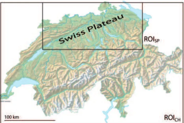
Fig. 1. Regions of interest used in this study covering the whole Switzerland (6◦E–10.5◦E, 45.75◦N–47.75◦N, ROICH) and the
polluted Swiss Plateau (7◦E–9.5◦E, 47◦N–47.75◦N, ROISP).
(Topographic map of Switzerland: © 2005 swisstopo).
reaction of NO2 with the OH radical. At night, a two step
reaction mechanism forms nitrogen pentoxide (N2O5) which
further reacts on surfaces and aerosol to HNO3(Dentener and
Crutzen, 1993). HNO3is finally removed by dry and wet
de-position (Kramm et al., 1995). Typical lifetimes of NOxare
of the order of 4 to 20 h depending on season (Seinfeld and Pandis, 1998). This is supported by results presented in this study inferred from the combination of SCIAMACHY NO2
VTCs with a high-quality NOxemission inventory. The
re-verse approach, that is the computation of NOx emissions
from satellite column observations based on a priori knowl-edge of NOxlifetimes or NO2column to NOxemission ratios
taken from a model, has recently become an important tool in top-down emission estimation for regions where sources are not well known (e.g. Martin et al., 2003).
Although the NOxconcentration in Switzerland decreased
during the last 15 years the Swiss NO2 annual ambient air
quality standard of 30 µgm−3 (≈16 ppb) is still exceeded in polluted areas (FOEN, 2005) and there has been a stag-nation or even a slight increase in NO2 in recent years
(Hueglin et al., 2006). Monitoring of nitrogen oxides there-fore plays an important role for the assessment of reduc-tion measures. Complementary to ground-based monitoring networks which provide detailed information of local near-surface air pollution, space-borne instruments such as the Global Ozone Monitoring Experiment (GOME) (Burrows et al., 1999) and the Scanning Imaging Absorption Spectrome-ter for Atmospheric Chartography (SCIAMACHY) (Bovens-mann et al., 1999) provide area-wide data of NO2
verti-cal tropospheric column densities (VTCs) with global cov-erage within a few days. The gradually improving res-olution of space-borne UV/VIS instruments (GOME pixel size: 320×40 km2, SCIAMACHY: 60×30 km2, occasion-ally 30×30 km2, Ozone Monitoring Instrument (OMI): up
to 13×24 km2 at nadir) increasingly allows to detect NO2
pollution features on a regional scale. However, these space-borne data and their complex retrieval are still recent and evolving techniques and validation is therefore needed. Schaub et al. (2006) summarised different validation cam-paigns of GOME and SCIAMACHY NO2 data and
car-ried out a detailed comparison of GOME NO2 VTCs
re-trieved by KNMI (Royal Dutch Meteorological Institute) and BIRA/IASB (Belgian Institute for Space Aeronomy) with NO2 profiles derived from ground-based in situ
measure-ments at different altitudes in the Alpine region.
In this paper we evaluate SCIAMACHY NO2VTCs over
Switzerland and the Alpine region with regard to their use for air quality monitoring and modelling on a regional scale and over a complex topography. The observations are com-pared to a high quality NOxemission inventory in order to
test the ability of SCIAMACHY to detect the distribution of NOx pollution sources on the scale of a small country. This comparison is further used to infer seasonal mean NOx
life-times carefully taking into account the influence of the strong diurnal cycle in NOxemissions on these estimates.
The significantly enhanced potential of SCIAMACHY as compared to the Global Ozone Monitoring Instrument GOME regarding the resolution of regional scale NOx
pol-lution features is demonstrated by a comparison of multi-annual mean distributions of the two instruments over Switzerland. In addition, mean seasonal cycles representa-tive for the Swiss Plateau are calculated for both instruments and compared to each other as well as to NO2columns
de-duced from ground-based in situ measurements carried out at different altitudes. From this comparison evidence is found that SCIAMACHY underestimates the amplitude of the sea-sonal cycle over the Swiss Plateau.
In the last part of this study the potential effects of the complex topography over the Alpine region on the retrieval are investigated. Based on a sensitivity analysis applied to selected SCIAMACHY pixels it is demonstrated that the use of a coarse resolution topography in the retrieval can indeed lead to significant systematic errors in NO2VTCs over the
Swiss Plateau. The results are relevant for any region of the globe with a marked orography and highlight the need for a more accurate representation of this parameter in future satel-lite retrievals.
2 Data
2.1 KNMI/BIRA GOME and SCIAMACHY tropospheric NO2observations
Nadir measurements from GOME on board ESA’s ERS-2 satellite and from SCIAMACHY on board ESA’s En-visat satellite are used in the present study. Depending on whether the focus is the whole domain of Switzerland or only the densely populated Swiss Plateau, our analyses will be
restricted to pixels with centre coordinates within the region of interest ROICHor ROISP, respectively (Fig. 1).
The GOME and SCIAMACHY observations are obtained at approximately 10:30 and 10:00 local time and individual pixels cover an area of 320×40 km2and 60×30 km2, respec-tively. The GOME and SCIAMACHY measurement prin-ciples are described in Burrows et al. (1999) and Bovens-mann et al. (1999), respectively. The NO2 VTCs
stud-ied in this work are the product of a collaboration between KNMI and BIRA/IASB. Both GOME and SCIAMACHY NO2 data are publicly available on a day-by-day basis via
ESA’s TEMIS project (Tropospheric Emission Monitoring Internet Service,www.temis.nl).
The first retrieval step is based on the Differential Opti-cal Absorption Spectroscopy (DOAS) technique (Platt, 1994; Vandaele et al., 2005): a polynomial and a modelled spec-trum are fitted to the logarithm of the ratio of earthshine ra-diance to solar irrara-diance in the spectral window from 426.3– 451.3 nm. The modelled spectrum accounts for spectral ab-sorption features of NO2, O3, O2-O2, H2O, and the
filling-in of Fraunhofer lfilling-ines by Raman scatterfilling-ing (“Rfilling-ing effect”). Scattering by clouds, aerosols, air molecules and the sur-face is described by a low-order polynomial. This first re-trieval step results in the slant column density (SCD) of NO2,
which can be interpreted as the column integral of absorbing NO2molecules along the effective photon path from the sun
through the atmosphere to the spectrometer.
The second retrieval step separates the stratospheric con-tribution from the total SCD (Boersma et al., 2004). For KNMI retrievals this is achieved with a data-assimilation approach using the TM4 global chemistry transport model (CTM) (Dentener et al., 2003). The tropospheric SCD (SCDtrop) results from the subtraction of the stratospheric
es-timate from the total SCD.
In the third retrieval step, the SCDtropis converted into a
VTC by applying the tropospheric air mass factor (AMFtrop).
Following Palmer et al. (2001) and Boersma et al. (2004), the retrieved SCIAMACHY NO2VTC (XSCIA) is calculated as
XSCIA= Ntrop Mtrop(xa, b) =Ntrop· P lxa,l P lml(b) · xa,l (1) where Ntrop denotes the tropospheric slant column density,
Mtrop the tropospheric air mass factor, xa,l the layer spe-cific subcolumns from the a priori profile xa, and ml the altitude-dependent scattering weights. These weights are cal-culated with the Doubling Adding KNMI (DAK) radiative transfer model (Stammes, 2001) and best estimates for for-ward model parameters b, describing surface albedo, cloud parameters (fraction, height) and pixel surface pressure. The a priori NO2profiles for every location and all times are
ob-tained from the TM4 CTM. Cloud fraction and height are taken from the Fast Retrieval Scheme for Clouds from the Oxygen A band (FRESCO) algorithm (Koelemeijer et al., 2001). Since the TM4 model is driven by meteorological data of the European Centre for Medium-Range Weather
Forecasts (ECMWF) the surface pressures in TM4 are taken from the ECMWF model on the 2◦×3◦ resolution of the TM4 model. The surface pressure for an individual satellite pixel is linearly interpolated to the pixel location (hereafter ECMWF/TM4 surface pressure).
The different error sources in tropospheric NO2retrievals
have been discussed extensively in Boersma et al. (2004) for GOME and error propagation studies have shown that SCIA-MACHY errors are similar (Boersma et al., 2007). Based on this work, errors for both GOME and SCIAMACHY NO2
VTCs are estimated on a pixel-to-pixel basis and addition-ally provided in the TEMIS data sets. However, these studies have not included the effect of errors in surface pressure. The present work will show that, over a complex topography, an inadequate treatment of this parameter may lead to signifi-cant errors which tend to be larger for an instrument with a higher spatial resolution such as SCIAMACHY as compared to GOME.
2.2 Swiss NOxemissions
Swiss NOx emissions amount to 33.2 kt N/y with traffic,
industry, agriculture/forestry and residential activities con-tributing 58%, 24%, 12% and 6%, respectively, for the year 2000 (FOEN, 2005). The present study employs an hourly resolved NOx emission inventory for Switzerland available
on a 3×3 km2grid. It combines the following basic data sets:
– Road traffic emissions of NOx for the reference year
2000 with a spatial resolution of 250 m prepared by the consulting company INFRAS, Switzerland. The data set includes an average diurnal variation. Long-term trends of annual totals recently published in Keller and Zbinden (2004) were used to interpolate the emissions between 2000 and 2005.
– NOx emissions from residential activities, heating,
in-dustry, off-road traffic and agriculture/forestry for the reference year 2000 with a spatial resolution of 200 m and accounting for seasonal variations prepared by the company Meteotest, Switzerland. Data sets for other years of interest were calculated on the basis of trends provided by the Swiss Federal Office for the Environ-ment (FOEN, 1995).
Additional information on the emission inventory is sum-marised in Keller et al. (2005). Total emission inventories are usually based on a large number of input variables. Each of these parameters – and, thus, also the resulting total emis-sion inventory – are affected by uncertainties. Their assess-ment is a challenging task which needs further assumptions (e.g. K¨uhlwein and Friedrich, 2000). For the 3×3 km2Swiss NOx emission inventory an accuracy of ±15–20% is
esti-mated in FOEN (1995). K¨uhlwein (2004) further pointed out increasing errors in emission inventories for increasing spatial resolutions. Thus, due to integration of the 3×3 km2
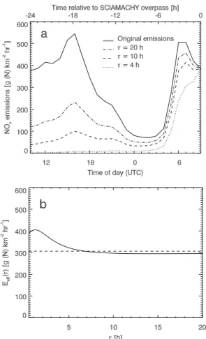
Fig. 2. Diurnal cycle of NOxemissions (in g (N) km−2h−1) over
Switzerland. The solid line is the hourly emission flux from the Swiss emission inventory (in winter) averaged over the domain of Switzerland. The three other lines illustrate the effect of the expo-nential decay of NOxfor three selected lifetimes τ . This decay leads
to a reduced contribution of the emissions released at a given time of the day to the NOxcolumn M measured at the SCIAMACHY
overpass time, see Eq. (5) (a). Effective NOxemission rate Eeffas
a function of lifetime τ . The dashed line is the daily mean emission rate (average of solid line if panel a) (b).
resolved emission data over the SCIAMACHY pixel size of 60×30 km2in the present work, the above given error of 20% is considered as a reasonable upper limit, which will be as-sumed in this study.
3 Methods
3.1 Comparison of NO2VTCs with a high resolution
emis-sion inventory for the estimation of mean NOxlifetimes
In Sects. 4.1.1 and 4.1.2 NO2VTCs will be compared to the
Swiss NOxemission inventory for SCIAMACHY pixels
lo-cated entirely within the Swiss boundaries. A representative emission rate is computed for each NO2VTC by averaging
the gridded inventory data over the area of the pixel. The
comparison is restricted to clear sky pixels (cloud fraction < 0.1) and anticyclonic conditions. Meteorological conditions are deduced from the Alpine Weather Statistics described in MeteoSwiss (1985). The Alpine Weather Statistics distin-guishes between advective and convective classes based on pressure gradients in surface charts. Anticyclonic conditions are a subset of the convective class and are characterized by fair weather and low surface level winds of typically less than 15 km/h. Significant long-range advection of air pollutants is unlikely to occur under these conditions, at least in the boundary layer. Therefore, a close association between the emission distribution and the NO2column field is expected.
The NOx emissions released at the location of the
col-umn are considered as the main flux of NOxinto the column
which, in an equilibrium state, is balanced by the chemical and physical (i.e. deposition) losses in the column. Neglect-ing transport and assumNeglect-ing first order losses only and steady state, we can write
dM
dt =E−k · M=0, (2)
with M the amount of NOxin the column (in g (N) km−2),
E the NOxemission flux (in g (N) km−2h−1), and k the first
order loss rate. Reforming yields M=1
k ·E=τ · E, (3)
with τ the lifetime of NOxin the column. The lifetime can
thus be obtained as the slope in a correlation plot of M versus E. In order to account for inaccuracies in both the observed columns and the emission rates, the slopes are calculated using weighted orthogonal regression (York, 1966). NOx
columns M are computed from the product of SCIAMACHY tropospheric NO2VTC and simulated NOx/NO2ratios, both
contributing to the error in M. The SCIAMACHY NO2
VTC 1σ error estimates are taken from the TEMIS data file where error estimates are provided for each individual pixel (Boersma et al., 2004). Errors introduced by the uncertainty in NOx/NO2column ratios are described later. For the NOx
emission fluxes averaged over the individual SCIAMACHY pixels an error of 20% is assumed (Sect. 2.2).
The basic assumption of steady state has also been made in earlier studies by Leue et al. (2001), Beirle et al. (2003) and Kunhikrishnan et al. (2004). It disregards the horizontal NOx
transport into and out of the column. This transport, however, can lead to a smearing because the net effect of transport will be negative for regions with large sources and positive for the surrounding areas. The smearing effect is also de-pending on the prevailing meteorology (e.g. wind speed and direction) and the chemical lifetime. For mapping isoprene emissions from space-borne data, Palmer et al. (2003) deter-mined typical smearing length scales. For NOxlifetimes in
the order of hours to one day, this length scale is ∼100 km (Martin et al., 2003). While neglecting the effect of trans-port is well justified for the large size of GOME pixels as
in the study of Martin et al. (2003), this might be problem-atic for SCIAMACHY data with a much smaller pixel size of 60×30 km2. However, as described above, our analysis is restricted to clear sky pixels and anticyclonic weather con-ditions associated with low wind speeds, i.e. rather stagnant air, and fast photochemistry reducing the importance of hor-izontal transport in the boundary layer. Significant transport over larger distances (e.g. from highly polluted regions in adjacent countries to Switzerland as described in Schaub et al. (2005) for a frontal passage) is therefore considered to be unimportant for theses conditions.
SCIAMACHY NO2 VTCs are converted to NOx VTCs
by employing representative values for the seasonal mean NO2/NO ratio. The latter depends on the abundance of ozone
and reactive organic compounds as well as on solar radiation and temperature. Thus, the ratio varies both spatially (hori-zontally and vertically) and seasonally. For the United States and based on 106 NOxmonitoring data sets measured at
dif-ferent distances from the predominant emission sources, Chu and Meyer (1991) recommended a national default value for the NO2/NO ratio of 3. NOx measurements operated since
1999 at an elevated rural site at the edge of the Swiss Plateau (Rigi, 47◦04′N, 8◦28′E, 1030 m a.s.l.) using a standard chemiluminescence detector for the measurement of NO and a photolytic converter for the selective conversion of NO2to
NO (Steinbacher et al., 2007) indicate a seasonal variation of monthly mean ratios of between 1.6 (January) and 4.0 (Au-gust) for anticyclonic clear sky conditions and a time win-dow between 10:00 and 12:00 UTC (Steinbacher, personal communication). Instead of using ratios from in-situ obser-vations valid only for the altitude of the measurement site, we here apply seasonal mean tropospheric (0–8 km) column NO2/NO ratios obtained from the TM4 model. The ratios
are based on model output over Switzerland on clear days. Unfortunately, only output for 12:00 UTC (13:00 LT) was available. Nevertheless, these TM4 column ratios are as-sumed to be representative for the SCIAMACHY overpass time (10:00 LT) and are found to be surprisingly close to the ratios observed in situ at Mount Rigi. Vertical model pro-files indicate that the NO2/NO ratio changes only little in
the lowest 1 to 2 km where most of the NO2resides, which
likely explains the good agreement with the ratios measured at a single altitude. Above the planetary boundary layer, the ratios decrease rapidly but the free troposphere contributes only little to the total column above Switzerland.
The ratios finally applied are 3.0 (±0.7) for spring (MAM), 4.0 (±0.6) for summer (JJA), 2.8 (±1.0) for au-tumn (SON), and 1.5 (±0.5) for winter (DJF), where values in brackets represent the 1σ variability of the column ratios between individual days. The uncertainty in these ratios is added to the uncertainty in the SCIAMACHY NO2VTC to
obtain an estimate for the uncertainty of the NOxVTCs M
finally used in the calculation of seasonal mean lifetimes ac-cording to Eq. (3). It is interesting to note that these ratios do not change significantly when cloudy days are included
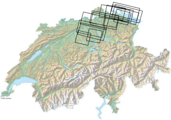
Fig. 3. Topographic map of Switzerland (© 2005 swisstopo) with the location of the SCIAMACHY pixels used for the pixel surface pressure sensitivity calculation.
in the analysis, probably due to the compensating effects of reduced photolysis rates (increasing the ratio) and at the same time reduced O3concentrations (reducing the ratio) on
cloudy days. Obtaining an emission rate E representative for the time of the SCIAMACHY overpass (10:00 LT cor-responding to 09:00 UTC over Switzerland) is not straight-forward due to the strong diurnal cycle in NOx emissions.
If NOxhas a short lifetime then only the emissions released
during a few hours preceding the satellite overpass contribute to the NO2 VTC measured by SCIAMACHY. If the
life-time is longer, however, then also emissions of the previous night and the previous day become relevant. This problem is illustrated in Fig. 2a showing the average diurnal cycle of NOxemissions over Switzerland in winter (solid line). Also
shown are the effective contributions of the emissions to the measured column if we assume three different NOxlifetimes
τ of 4, 10, and 20 h (dotted and dashed-dotted lines). The problem can be formulated as follows: The amount of NOxreleased at a given hour ti of the day over a period 1t =1 h (i.e. Ei·1t , where Ei is the emission rate at hour i given by the solid line in Fig. 2a) decays exponentially with a time constant τ . The column amount M accumulated by all emissions released during n-hours preceding the overpass can thus be expressed as:
M= n X i=1 Ei·e −(tSCIA−ti ) τ ·1t , (4)
where tSCIA−ti is the time difference between the SCIA-MACHY overpass and the NOxrelease in hours. Values of
Eiexp(−(tSCIA−ti)/τ ) are shown in Fig. 2a for three differ-ent lifetimes τ . Combining this equation with Eq. (3) we can compute an effective emission rate Eeff relevant for a given
200 400 600 800 1000 height [hPa] NO2 sub columns [10 15 molec cm-2 ] TM4 surface pressure effective surface pressure
0.8 0.6 0.4 0.2 0 1.0 NO2 sub columns [10 15 molec cm-2 ] 0.8 0.6 0.4 0.2 0 1.0 proile a proile b
Fig. 4. CTM a priori NOx profiles (a) (poor vertical
mix-ing/polluted) and (b) (strong vertical mixing/remote) given as layer-specific sub columns. The black profiles are associated with the ECMWF/TM4 surface pressure at the location of the SCIAMACHY pixel. The red profiles are reaching down to the effective surface pressure calculated from the aLMo model with a 7×7 km2 resolu-tion. For the examples shown here, surface pressures are taken from 10 March 2004 (profile a) and from 21 July 2001 (profile b).
lifetime τ as Eeff(τ )= Pn i=1Ei·e −(tSCIA−ti ) τ ·1t τ . (5)
Defining the weights wi=exp(−(tSCIA−ti)/τ ) and noting that the sumPiwi·1t =τ we can rewrite Eq. (5) as Eeff(τ )= Pn i=1Ei·wi Pn i=1wi . (6)
The effective emission rate is thus a weighted mean of the original emissions with weights given by an exponential de-cay with time constant τ . Values of Eeffare shown in Fig. 2b
as a function of lifetime τ . For comparison, the daily mean emission rate is also shown (dashed line). For short lifetimes lower than about 7 h the effective emission rate is higher than the daily mean because only the high morning emis-sions including the early morning traffic peak are relevant. For longer lifetimes the low emission rates of the previous night become important reducing Eeffbelow the daily mean
value. It is important to notice that the effective emission rate depends not only on the NOxlifetime but also on the time of
the satellite overpass. Such complicating effects need to be carefully considered for instance in NOxemission inversion
studies using a combination of model information and satel-lite observations to obtain improved emission estimates.
Now we are facing the problem that, for the calculation of lifetime τ according to Eq. (3), we have to use an effective emission rate which itself is depending on τ . This problem can be solved iteratively with
τi=M/Eeff(τi−1), (7)
where in each step (i) the emission Eeff is adjusted to the
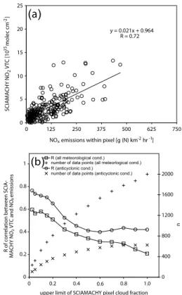
lifetime obtained from the previous step (i−1) using Eq. (6). The iteration is found to converge quickly within no more than 4 steps. Lifetime estimates based on this approach will be presented in Sect. 4.1.2. y = 0.021x + 0.964 R = 0.72 0 5 10 15 20 25
NOx emissions within pixel [g (N) km-2 hr-1]
SCIAMACHY NO 2 VTC [10 15 molec cm -2] 0 125 250 375 500 625 750
(a)
0 400 800 1200 1600 2000 nR (all meteorological cond.) R (anticyclonic cond.)
number of data points (all meteorlogical cond.) number of data points (anticyclonic cond.)
0 0.2 0.4 0.6 0.8 1
upper limit of SCIAMACHY pixel cloud fraction
R of correlation between
SCIA-MACHY NO2 VTC and NO emissions
0 0.2 0.4 0.6 0.8 1.0
x
(b)
Fig. 5. Comparison between SCIAMACHY NO2 VTCs (from
2003–2005) and collocated 09:00–10:00 UTC NOxemission rates
for pixels located entirely within the Swiss boundaries and anti-cyclonic clear sky meteorological conditions (pixel cloud fraction
≤0.1 n=243) (a). Correlation coefficients of the present compari-son as a function of different cloud fraction thresholds (b).
3.2 Sensitivity of SCIAMACHY NO2 VTCs to varying
pixel surface pressure
As mentioned in Sect. 2.1 the mean pixel surface pressure is one of the parameters used in the column retrieval. In the TEMIS product this parameter is taken from the TM4 model to be consistent with the a priori NO2 profile. It
is therefore only available on a coarse resolution of 2◦×3◦ (∼220×240 km2) not resolving the complex topography of the Alpine region. The potential effects of this smoothed to-pography on NO2 column retrievals over Switzerland will
be demonstrated in Sect. 4.3 in terms of a sensitivity anal-ysis. The following methods will be applied: For GOME and SCIAMACHY pixels with centre coordinates within the region of interest ROICH (Fig. 1) the deviations from
the true topography are quantified. For this purpose the ECMWF/TM4 surface pressures psurf are converted to
al-titude hsurf using daily profiles of pressure derived from
ground based measurements at different altitudes in Switzer-land. These values are then compared to the pixel averaged effective altitude heff based on the high resolution
topogra-phy of the aLMo model (Alpine Model, the MeteoSwiss nu-merical weather prediction model) available on a resolution of 7×7 km2.
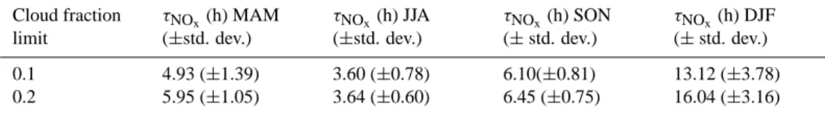
Table 1. Seasonal NOxlifetime estimates based on a weighted orthogonal regression and lifetime-dependent effective emission rates for two
different cloud fraction limits. Stated uncertainties correspond to the standard deviations of the slopes determined by the regression. Cloud fraction limit τNOx(h) MAM (±std. dev.) τNOx (h) JJA (±std. dev.) τNOx(h) SON (± std. dev.) τNOx(h) DJF (± std. dev.) 0.1 4.93 (±1.39) 3.60 (±0.78) 6.10(±0.81) 13.12 (±3.78) 0.2 5.95 (±1.05) 3.64 (±0.60) 6.45 (±0.75) 16.04 (±3.16)
The sensitivity study is then carried out for a subset of clear sky SCIAMACHY pixels and two fixed a priori NO2
profiles only. The AMFtrop and NO2 VTCs are first
cal-culated for the ECMWF/TM4 surface pressure psurf as in
the original retrieval and then recalculated for the effective surface pressure peff deduced from the aLMo topography
heff using again the ground based vertical pressure profiles.
The criteria for the pixel subset are i) anticyclonic clear sky meteorological conditions (Alpine Weather Statistics; Me-teoSwiss, 1985), ii) pixel cloud fraction ≤0.1, and iii) a small standard deviation <65 m of the aLMo 7×7 km2 grid cell heights enclosed within a SCIAMACHY pixel, the latter en-suring that the reprocessing is done for pixels over a flat re-gion in the vicinity of the Alps rather than directly over the mountains. The resulting SCIAMACHY pixels are located above the rather flat north-eastern Swiss Plateau (Fig. 3) but their surface pressure psurfis still strongly influenced by the
proximity of the Alps at the coarse ECMWF/TM4 resolution. The sensitivity analysis is performed for two characteris-tic (and fixed) CTM a priori NO2profile shapes (Fig. 4). In a
first profile (a), the bulk of NO2is residing near the ground.
This profile is applied to pixels sampled during the cold part of the year (November-March) as it is expected to occur over polluted regions during the winter months when vertical mix-ing is generally weak or non-existmix-ing. The second profile (b) is applied to the subset of SCIAMACHY pixels sampled be-tween April and August. It shows a much lower NO2
abun-dance near the ground representing either a profile over a remote location or a summertime profile resulting from en-hanced vertical mixing. As shown in Fig. 4 the use of a different surface pressure scales the profile vertically. The other retrieval (or forward model) parameters including sur-face albedo, cloud fraction and height, solar zenith angle and so on are kept constant.
4 Results and discussion
4.1 SCIAMACHY NO2 VTCs versus NOx emissions in
Switzerland
4.1.1 Qualitative comparison
Figure 5a shows the comparison between SCIAMACHY NO2 VTCs and the corresponding 09:00–10:00 UTC NOx
emission rates for anticyclonic clear sky (cloud fraction ≤0.1) conditions together with a simple linear regression (n=243). This simple comparison is limited by a number of factors: The relation between NO2VTCs and the
corre-sponding NOxemissions is expected to change with
differ-ent meteorological conditions which influence the lifetime of NOxas well as the NOx/NO2column ratio. Even though
the comparison is restricted to anticyclonic conditions, some transport of NOxinto and out of the column may still make
a non-negligible contribution to the column budget. In addi-tion, using emission rates from a fixed release time interval is not the best possible choice as discussed in Sect. 3.1.
Nevertheless, the resulting correlation coefficient of R=0.72 indicates that the collocated emissions explain more than 50% of the variance in the NO2 VTCs. From this
we may conclude that SCIAMACHY is able to observe the sources of air pollution from space even though its sensitivity is strongly decreasing towards the earth’s surface.
Figure 5b shows the sensitivity of the correlation coeffi-cient to the upper limit selected for the cloud fraction; i.e., only SCIAMACHY pixels with cloud fractions lower than or equal to this limit are taken into account. The compar-ison is carried out for all meteorological conditions (square symbols) as well as for anticyclonic conditions only (circles). The better correlations for the anticyclonic cases support our hypothesis that transport effects play a much smaller role un-der these conditions which are typically characterized by low wind speeds and rather homogeneous air masses (e.g. no pas-sages of fronts). The general trend of decreasing correla-tions with increasing cloud fraction thresholds can be under-stood from clouds screening NO2located below. Moreover,
in cloudy situations, the retrieved column is more strongly af-fected by the a priori assumption for the vertical NO2profile
as was shown by Schaub et al. (2006). Note that the levelling off of the correlation coefficients for high upper cloud frac-tion limits in Fig. 5b is mainly due to the small number of cases that are additionally taken into account (denoted by the number of data points additionally shown in Fig. 5). 4.1.2 NOxlifetime under anticyclonic clear sky conditions
As described in Sect. 3.1 the NOxlifetime can be deduced
from the slope of a correlation plot of NOxcolumns M versus
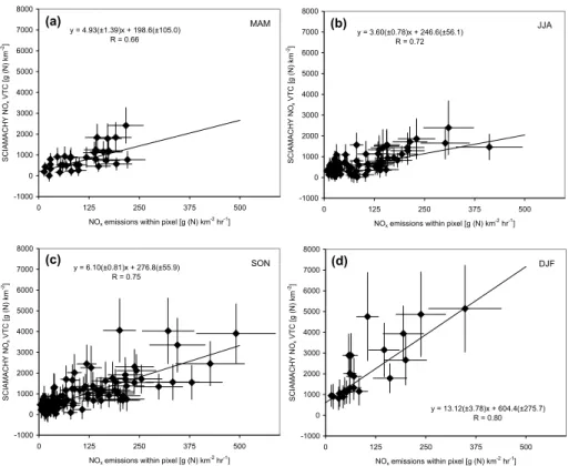
y = 4.93(±1.39)x + 198.6(±105.0) R = 0.66 -1000 0 1000 2000 3000 4000 5000 6000 7000 8000 0 125 250 375 500
NOx emissions within pixel [g (N) km -2 hr-1 ] SC IAM A C H Y N Ox V T C [ g (N ) km -2] MAM (a) y = 3.60(±0.78)x + 246.6(±56.1) R = 0.72 -1000 0 1000 2000 3000 4000 5000 6000 7000 8000 0 125 250 375 500
NOx emissions within pixel [g (N) km -2 hr-1 ] SC IAM A C H Y N Ox V T C [ g (N ) km -2] JJA (b) y = 6.10(±0.81)x + 276.8(±55.9) R = 0.75 -1000 0 1000 2000 3000 4000 5000 6000 7000 8000 0 125 250 375 500
NOx emissions within pixel [g (N) km -2 hr-1 ] SC IAM A C H Y N Ox V T C [ g (N ) km -2] SON (c) y = 13.12(±3.78)x + 604.4(±275.7) R = 0.80 -1000 0 1000 2000 3000 4000 5000 6000 7000 8000 0 125 250 375 500
NOx emissions within pixel [g (N) km-2
hr-1 ] SC IAM A C H Y N Ox V T C [ g (N ) km -2] DJF (d)
Fig. 6. Clear sky (cloud fraction≤0.1) SCIAMACHY NOxVTCs located entirely within the Swiss boundaries versus iteratively calculated
effective NOxemission rates Eeff, see Eq. (7) for the four seasons spring (a), summer (b), fall (c) and winter (d). NOxVTCs are calculated
from observed NO2VTCs using seasonal mean NO2/NO column ratios. Additionally, the orthogonal regression output accounting for errors
in both regression parameters is given. The slopes are the seasonal mean NOxlifetimes in hours (see also Table 1).
suitable units. Instead of using emission rates from a fixed time interval as in the previous section, effective emission rates Eeff are used in the following calculated according to
the iterative method described in Sect. 3.1.
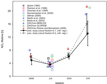
The seasonal mean lifetimes are summarised in Table 1 and shown in Fig. 7 together with other estimates based on published data.
For summer, a large number of estimates is available
– from measurements in power plant plumes: 5 h
(Ryer-son et al., 1998), 2.8 and 4.2 h (Nunnermacker et al., 2000) and 6.4 h (Sillman, 2000),
– from measurements in urban plumes: Boston: 5.5 h
(Spicer, 1982), Nashville: 2.0 h (Nunnermacker et al., 2000), Zurich: 3.2 h (Dommen et al., 1999),
– from GOME NO2VTCs above Germany: 6.0 h (Beirle
et al., 2003) and
– zonal mean in the boundary layer (0–2 km) from the
GEOS-CHEM CTM: 3.0 h (Martin et al., 2003). For spring, Martin et al. (2003) calculated a mid-latitude NOxlifetime from the GEOS-CHEM model of 8 h. For the
winter season, Martin et al. (2003) and Beirle et al. (2003) reported on NOxlifetimes of 19 and 21 h, respectively.
Additional NOx lifetimes have been estimated here for
the main daytime loss mechanism which is the oxidation of NO2 by OH to form HNO3. These estimates are based
on pressure (∼960 hPa) and temperature values representa-tive for the Swiss Plateau and on OH concentrations taken from the BERLIOZ and the SLOPE96 campaigns as well as from long-term OH measurements carried out at Hohen-peissenberg. The BERLIOZ campaign took place at a dis-tance of 50 km from Berlin; the SLOPE96 campaign fo-cused on polluted air masses travelling from the city of Freiburg to the Schauinsland Mountain (south-western Ger-many); the Hohenpeissenberg station is located in South-ern Germany at an altitude of 985 m a.s.l. From a pollu-tion point of view, all regions are similar to the condipollu-tions encountered over the Swiss Plateau. For an assumed tem-perature of 298 K and based on OH concentrations taken from the BERLIOZ and the SLOPE96 campaigns with noon-time values of (4–8)×106cm−3(Volz-Thomas et al., 2003; Mihelcic et al., 2003) and (7–10)×106cm−3(Volz-Thomas and Kolahgar, 2000), respectively, the resulting mean day-time NOxlifetimes in summer are estimated to be 4.6 h and
3.0 h. Seasonally averaged 09:00–10:00 UTC OH concen-trations determined from clear sky OH measurements at Ho-henpeissenberg carried out between 1999 and 2005 (Rohrer
0 4 8 12 16 20 season N Ox l if e ti m e [ h ] Spicer (1982) Ryerson et al. (1998) Dommen et al. (1999) Nunnermacker et al. (2000) Sillman (2000) Martin et al. (2003) Beirle et al. (2003) [OH] from BERLIOZ [OH] from SLOPE96
[OH] from Rohrer and Berresheim (2006) pres. study (cloud fraction<0.1, orth. regr.) pres. study (cloud fraction<0.2, orth. regr.)
MAM JJA SON DJF
Fig. 7. Seasonal NOxlifetimes (and standard deviations) over the
Swiss Plateau under anticyclonic clear sky conditions estimated in this study. Results from other studies are shown for comparison. These data have been deduced from campaigns in the U.S. (Spicer, 1982; Ryerson et al., 1998; Nunnermacker et al., 2000; Sillman, 2000) and in the Swiss Plateau (Dommen et al., 1999), from GOME NO2VTCs over Germany (Beirle et al., 2003) and from the
GEOS-CHEM model (Martin et al., 2003). Additionally, mean NOx
life-times against oxidation to HNO3are calculated for (i) 960 hPa and
298 K with OH concentrations of (4–8)×106cm−3measured dur-ing the BERLIOZ campaign (Volz-Thomas et al., 2003; Mihelcic et al., 2003) and of (7–10)×106cm−3measured during the SLOPE96 campaign (Volz-Thomas and Kolahgar, 2000) as well as for (ii) seasonally averaged OH concentrations measured by Rohrer and Berresheim (2006) with 960 hPa and assumed temperatures for the summer, spring/fall and winter seasons of 298 K, 288 K and 278 K, respectively.
and Berresheim, 2006; Berresheim, unpublished data, 2006) are used together with assumed temperatures for summer, spring/fall and winter of 298 K, 288 K and 278 K, respec-tively, to estimate NOxlifetimes of 6.1, 3.9, 8.2 and 21.0 h
for MAM, JJA, SON and DJF, respectively (Fig. 7).
Figure 6 shows for each season the SCIAMACHY NOx
columns for anticyclonic clear sky conditions plotted against the corresponding effective NOxemission rates Eeff.
Addi-tionally, the linear fits obtained by the weighted orthogonal regression are shown. The relatively small intercepts sug-gest that under anticyclonic conditions the background NOx
plays a rather marginal role and the SCIAMACHY observa-tions are dominated by the local NOxemissions. The slopes
of the linear fits correspond to the seasonal mean lifetimes. The effective emission rates used in the figure optimally cor-respond to these lifetimes as assured by the iterative adjust-ment (Eq. 7).
The comparison of our NOxlifetimes with independent
es-timates generally shows a reasonable agreement though our values tend to be at the lower end, in particular in winter.
A possible reason is that our estimates are only valid for clear sky situations. In Fig. 7 the dashed line shows addi-tional lifetimes calculated for a higher cloud fraction limit of 0.2. For this higher threshold all lifetimes become larger (see also Table 1). The uncertainty ranges, on the other hand, become smaller because a larger number of data points can be included in the calculation of the slopes. A higher cloud fraction reduces the amount of solar radiation reaching the boundary layer. This in turn decreases the OH concentra-tions (Rohrer and Berresheim, 2006) which likely explains the larger lifetimes for the higher threshold. The Hohenpeis-senberg OH data have been obtained for clear sky days with cloud fractions ≤1 octa (0.125), too. However, the winter-time lifewinter-time estimate is significantly higher than the SCIA-MACHY based estimate for a comparable cloud fraction of 0.1. This may be an indication that nighttime conversion to HNO3and deposition may be more important losses of NOx
in winter than reaction with OH during daytime. The lifetime estimates of Martin et al. (2003) represent monthly mean val-ues not restricted to clear sky days. There is no obvious dis-crepancy from our estimates assuming that our values would become larger if even higher cloud fractions would be al-lowed.
All other estimates are implicitly representing clear sky or at least fair weather conditions, too. The different sum-mertime estimates, for instance, were obtained in the frame-work of studies dedicated to the investigation of photochem-ical ozone production focussing on sunny days, or were de-rived from clear sky satellite observations. Our summertime value of about 3.6 h is well in the range of these estimates. In particular, it is in excellent agreement with another study carried out over Switzerland by Dommen et al. (1999) which obtained a lifetime of 3.2 h (Fig. 7).
Neglecting horizontal transport (smearing effect) could also contribute to an underestimation of lifetimes using our approach. Even though we are focussing on anticyclonic conditions, transport effects may still play a role in partic-ular during winter when a long lifetime (>10 h) allows for transport over distances larger than the extension of SCIA-MACHY pixels despite low wind speeds (<15 km/h). 4.2 Comparison of GOME and SCIAMACHY NO2VTCs
over Switzerland
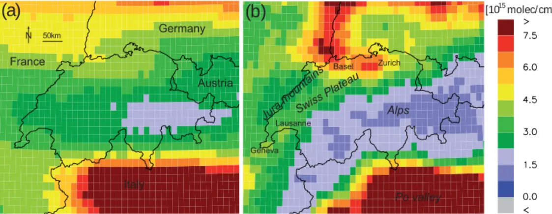
SCIAMACHY can better resolve regional structures of air pollution over Switzerland than GOME owing to the much smaller pixel size. This is demonstrated by Fig. 8 showing multi-annual mean NO2VTC distributions from (a) GOME
(1996–2003) and (b) SCIAMACHY (2003–2005) mapped onto a fine 0.125◦×0.125◦grid. For each grid cell a mean VTC has been computed by averaging over all clear sky pixels covering the given cell. Whereas the SCIAMACHY data can resolve the large contrast between the Alpine region (blue shadings) and the Swiss Plateau these differences are smeared out in the GOME data. In addition, SCIAMACHY
Italy France Germany Austria 50km N
(a)
Alps Jura mo unta ins Geneva Lausanne Basel Zurich Swiss Platea u Po valley [10 molec/cm ]15 2(b)
Fig. 8. Mean clear sky (satellite pixel cloud fraction ≤0.1) NO2tropospheric columns over the Central Alps and Switzerland deduced from
GOME (1996–2003) (a) and SCIAMACHY (2003–2005) retrievals (b). In contrast to the GOME picture, specific features such as the Alpine chain, the Jura Mountains, the Swiss Plateau and the areas of Greater Zurich and Basel clearly show up in the SCIAMACHY data.
can “see” individual population centres such as the areas of Zurich, Basel or the Rhine valley along the border between France and Germany. Elevated values are also seen around the cities of Lausanne and Geneva. All these details are miss-ing in the GOME data. Interestmiss-ingly, the area of Berne does not stand out even in the SCIAMACHY data, possibly due to the specific location of this city in between the Jura Moun-tains and the Alps.
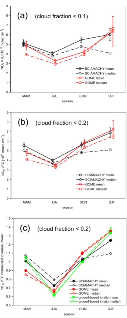
For a more quantitative comparison seasonally averaged GOME and SCIAMACHY NO2VTCs have been calculated
from all clear sky pixels with centre coordinates located within the region ROISP(see Fig. 1) covering the polluted
re-gions of the Swiss Plateau (7◦E – 9.5◦E, 47◦N – 47.75◦N) only. Restricting the comparison to this region reduces the influence of the complex Alpine terrain as much as possi-ble, which is particularly relevant for the large GOME pixels (Schaub et al., 2006). In Fig. 9a the resulting SCIAMACHY NO2VTCs are on average higher than the GOME columns
in spring, summer and autumn. Somewhat higher values can be expected for SCIAMACHY because the extended GOME pixels always include less polluted regions outside of the Swiss Plateau. Surprisingly, the SCIAMACHY wintertime values are lower than the ones from GOME, the difference being more pronounced for the median than for the mean values. However, the GOME value in winter is only based on 7 individual pixels. Anticyclonic conditions are typically associated with the formation of fog over the Swiss Plateau during winter which likely explains the poor availability of clear sky pixels.
In order to improve the statistics the cloud fraction thresh-old has been relaxed to 0.2 in Fig. 9b. For this threshthresh-old a reasonable sample size of 32 pixels is available in win-ter. The differences between SCIAMACHY and GOME be-come significantly smaller in this case, not only in winter. The relative amplitude of the seasonal cycle (winter max-imum – summer minmax-imum), however, remains about 25% lower in the SCIAMACHY data as compared to GOME as
highlighted in panel (c) where the values are scaled to the an-nual average. Again, the differences are more pronounced for the median values which are thought to be a more robust quantity as they are less susceptible to outliers.
For comparison, seasonally averaged NO2 columns
es-timated from NO2 data measured in situ between January
1997 and June 2003 at 15 ground-based sites at different al-titudes in Switzerland and Southern Germany are also shown in Fig. 9c. The elevated sites are assumed to detect NO2
con-centrations representative for the appropriate height in the (free) troposphere over flat terrain. These measurements, together with boundary layer in situ measurements and an assumed mixing ratio of 0.02 ppb at 8 km, are used to con-struct NO2 profiles. The latter are subsequently integrated
to tropospheric NO2 columns. Details on the data set and
method are given in Schaub et al. (2006). For the present study, the ground-based in situ data set has been restricted to all clear sky days as flagged by the sunshine and high fog parameters from the Alpine Weather Statistics (MeteoSwiss, 1985). The columns are reaching down to an assumed mean Swiss Plateau height of 450 m a.s.l. The normalised seasonal variation of the ground-based data agrees reasonably well with the variation observed by GOME, in particular regard-ing the large differences between summer and winter. Sim-ilarly pronounced seasonal variations of space-borne NO2
VTCs over industrialised regions have also been reported by Petritoli et al. (2004), Richter et al. (2005), van der A et al. (2006) and Uno et al. (2006). The seasonal amplitude in the SCIAMACHY data, however, is lower than in both GOME and ground-based observations: For the median val-ues the amplitude is reduced by more than a factor of two. For the means the reduction is about 25% as mentioned ear-lier. This suggests that SCIAMACHY values over the Swiss Plateau are possibly underestimated in winter and/or over-estimated in summer. It is important to note that this con-clusion is only drawn here for the specific KNMI/BIRA re-trieval. As has been shown by van Noije et al. (2006) there
0 1 2 3 4 5 6 7 8 9 N O2 VT C [ 1 0 15 mo le c cm -2] SCIAMACHY mean SCIAMACHY median GOME mean GOME median
(a)
(cloud fraction < 0.1)MAM JJA SON DJF
season 0 1 2 3 4 5 6 7 8 9 N O2 VT C [ 1 0 15 mo le c cm -2] SCIAMACHY mean SCIAMACHY median GOME mean GOME median
(b)
(cloud fraction < 0.2)MAM JJA SON DJF
season 0.5 0.6 0.7 0.8 0.9 1 1.1 1.2 1.3 1.4 1.5 N O2 V T C n o rma lis e d t o a n n u a l me a n SCIAMACHY mean SCIAMACHY median GOME mean GOME median ground-based in situ mean ground-based in situ median
(c)
(cloud fraction < 0.2)MAM JJA SON DJF
season
Fig. 9. Seasonal mean and median NO2VTCs from GOME and SCIAMACHY over the ROISP(Fig. 1) for cloud fractions ≤0.1.
76, 175, 129 and 86 SCIAMACHY pixels and 52, 95, 33 and 7 GOME pixels were available for the four seasons MAM, JJA, SON and DJF, respectively (a). Same as above but for cloud fractions
≤0.2. Number of SCIAMACHY pixels per season: 144, 256, 236, and 141; GOME: 106, 154, 88, 32 (b). Seasonal mean and median NO2VTCs from GOME, SCIAMACHY, and derived from ground-based in situ NO2 measurements normalised to the annual mean
value. Ground-based in situ columns were calculated following the method and data set described in Schaub et al. (2006) and for a Swiss Plateau ground elevation of 450 m a.s.l.. Number of in situ columns per season: 139, 165, 69 and 78 (c).
are substantial differences in seasonal variations obtained by different groups using different retrieval algorithms. More-over, our analysis is limited by the fact that SCIAMACHY and GOME have been sampled differently in space and time
Alps Swiss Plateau real topography model topography SCIAMACHY GOME SCIAMACHY
Fig. 10. Illustration of the problem arising for highly resolved satel-lite pixels over a marked topography when retrieved with coarsely resolved input parameters. The red and blue lines denote the aver-aged real surface height at the location of individual SCIAMACHY and GOME pixels, respectively. Further, the real topography and the topography given in a coarsely resolved global model are indi-cated. Over the large GOME pixel extension, the mean height given by a coarsely resolved model better approximates the averaged real surface height than for the smaller SCIAMACHY pixels.
and, thus, a perfect agreement is not expected. Nevertheless, the reduced seasonal cycle in SCIAMACHY data may be re-lated to a problem in the retrieval over complex orography discussed in the next section.
4.3 Influence of inadequate treatment of Alpine surface to-pography on NO2VTC retrievals
4.3.1 GOME and SCIAMACHY pixel surface pressures Errors of GOME NO2 VTC retrievals were initially
dis-cussed by Richter and Burrows (2002) and Boersma et al. (2004). The methods and error budgets of the TEMIS re-trievals applied to GOME, SCIAMACHY and OMI data are described in more detail in Blond et al. (2007) and Boersma et al. (2007). They reported on the following retrieval param-eters inducing inaccuracies in the AMF calculation, which is the major error source for tropospheric retrievals over polluted regions: the a priori NO2 profile shape, the
sur-face albedo, cloud characteristics (fraction and height) and aerosol concentration. Here, we propose an additional source for systematic errors only relevant over complex topography: the mean surface pressure (or height) assumed for the re-trieval of an individual pixel. This influence has not been in-vestigated in the literature so far. As discussed in Sect. 3.2 the surface pressure psurfused in the retrieval is obtained from
the TM4 model at coarse resolution (ECMWF/TM4 surface pressure). While for large parts of the globe this will be suf-ficiently accurate, the low resolution may lead to problems over complex topography such as the Alpine region, in par-ticular if there is a large mismatch in resolution between the satellite pixels and the surface pressure data set.
This is illustrated in Fig. 10 for the situation over the Alpine region. In a coarsely resolved model, the topography is averaged over extended grid elements, typically leading to an underestimation of the effective elevation of mountains
0 200 400 600 800 1000 -2200-2000-1800-1600-1400-1200-1000 -800 -600 -400 -200 0 200 400 600 800 hsurf-hef [m]
number of GOME pixels (total 5382)
(a)
0 200 400 600 800 1000 -2200-2000-1800-1600-1400-1200-1000 -800 -600 -400 -200 0 200 400 600 800 hsurf-hef [m]number of SCIAMACHY pixels (total 7808)
(b)
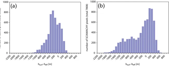
Fig. 11. Histogram distribution of the differences hsurf−heffbetween pixel surface heights used in the retrieval and effective surface heights
averaged over the pixels for all GOME (1996–2003) (a) and SCIAMACHY (2003–2005) (b) pixels with centre coordinates within ROICH
(Fig. 1).
and an overestimation of the effective ground height in the surrounding area. Because the size of SCIAMACHY pixels is much smaller than the size of a model grid cell, it can be expected that the mean model heights hsurf(thin dotted line)
show a larger deviation from the effective pixel-averaged sur-face heights hefffor the smaller SCIAMACHY pixels (thick
red lines) than for GOME (thick blue line).
Figure 11 presents histograms of the differences 1surf=hsurf−heff between ECMWF/TM4 based surface
elevations hsurf and effective heights heff for all GOME
pixels of the years 1996–2003 and SCIAMACHY pixels of the years 2003–2005 (b) over the domain ROICH (Fig. 1).
Figure 12 displays the corresponding pixel centre loca-tions color-coded by the values of 1surf. The following conclusions can be drawn:
– Due to the smoothed topography in ECMWF/TM4, the
surface heights of the GOME and SCIAMACHY pixels are underestimated over the Alps and overestimated over the Swiss Plateau (Fig. 12).
– Lower minimum and higher maximum values of 1surf
are found for SCIAMACHY pixels (Figs. 11 and 12). This can be expected due to the smaller pixel size of SCIAMACHY compared to GOME (Fig. 10).
This demonstrates that certain retrieval parameters, such as the mean pixel surface pressure, can become increasingly in-accurate with increasing resolution of the satellite data if the spatial resolution of the parameters is not improved accord-ingly. In the following section, the effect of an inaccurate pixel surface pressure on the resulting NO2VTC is
investi-gated for selected SCIAMACHY columns.
4.3.2 Sensitivity study for selected SCIAMACHY pixels Figure 13 shows an idealized NO2 profile over the Swiss
Plateau where hsurf>heff. The profile which would be used
in the retrieval reaching down to pressure psurfis shown in
black, the profile scaled to the higher effective surface pres-sure peff in red. Over the Alps the situation would be
re-versed. Following Eq. (1) (Sect. 2.1) and the formulation for the AMFtropgiven there, the following systematic errors due
to inaccurate surface heights are expected:
– For positive 1surf (hsurf>heff; e.g. over the Swiss
Plateau, Figs. 12) the near-ground NO2pollution is in
reality located at a lower level than assumed in the re-trieval. The retrieval therefore associates the high near-ground pollution with a too high sensitivity (thin dotted line in Fig. 13). This leads to an overestimated AMFtrop
and, thus, to an underestimated NO2VTC.
– For negative 1surf (hsurf<heff, e.g. over the Alps,
Fig. 12) a tendency towards overestimation of the NO2
VTCs is expected.
The effect of inaccurate pixel surface pressures is inves-tigated for selected SCIAMACHY pixels following the method described in Sect. 3.2. Table 2 presents an overview of the selected pixels and the results obtained by the sensi-tivity analysis. For the selected pixels over the northeastern Swiss Plateau (see Fig. 3) the surface pressures psurfand peff
differ by about 50 hPa, corresponding to about 450 m. The mean relative change in the AMFtropdue to the
chang-ing pixel surface pressure is −27.2±1.3% and −11.7±1.8% for the profile shapes A and B (Fig. 4), respectively. The mean relative change in the resulting NO2 VTCs is
(a)
-1400 -1200 -1000 -800 -600 -200 -400 0 200 400 600 hsurf -hef f [m](b)
Fig. 12. Differences between pixel surface heights used in the retrieval and effective surface heights averaged over the respective pixels (hsurf−heff) for all GOME (1996–2003) (a) and SCIAMACHY (2003–2005) (b) pixels located over ROICH(Fig. 1). The (hsurf−heff) value
for a pixel is indicated at its corresponding centre coordinate.
changes in the AMFtropand the NO2VTCs due to changes in
the pixel surface pressure are strongly dependent on the NO2
profile shape.
These results are only a first attempt at quantifying these effects based on a limited subset of SCIAMACHY pixels and assumed a priori profile shapes. Depending on the NOx
emis-sions taking place at the pixel location, photochemical activ-ity and prevailing meteorological conditions, real NO2
pro-file shapes will differ from the ones used here. Nevertheless, given the distinctly different shapes A and B, the 13–38% NO2 VTC error range appears to be a reasonable first
esti-mate. For retrievals in the UV-visible spectral range with a significant decrease of the sensitivity towards the earth’s surface, this effect is of major importance when the NO2
re-sides close to the ground. As this situation most prominently occurs during the cold season this probably leads to an un-derestimation of NO2 VTCs in winter and less so in other
seasons. Hence, the reduced seasonal amplitude in SCIA-MACHY data identified in Sect. 4.2 may be at least partly related to this problem.
At first glance, the problem seems to be less relevant for GOME as differences between true pressures and those used in the retrieval are smaller (Fig. 12a). Nevertheless, the com-plex topography over Switzerland probably leads to signifi-cant systematic errors, too. The reason is that NO2will not
be evenly distributed within a GOME pixel covering parts of the Swiss Plateau and the Alps as in Fig. 10. Most of the measured NO2signal will originate from that part of the pixel
located above the polluted Swiss Plateau for which there is still a discrepancy between true and ECMWF/TM4 altitude. If the contribution to the signal of the clean elevated part of the pixel would be zero then the relative error would be the same as for a SCIAMACHY pixel located entirely over the polluted part. However, since NO2VTCs over the Jura
mountains and pre-Alps are well above zero there will prob-ably be some compensation of the error since for these ele-vated regions the errors will be smaller or of opposite sign.
2 sensitivity (decreasing towards earth surface) 2 SCIAMACHY pixel surface height (psurf)
Effective
surface height (peff)
CTM NO profile for psurf CTM NO profile for psurf
Fig. 13. Possible reason for too low SCIAMACHY NO2VTCs
over the polluted Swiss Plateau: retrieval errors due to inaccurate pixel surface heights in regions with a marked topography.
5 Summary and conclusions
This study has evaluated SCIAMACHY NO2 VTCs above
Switzerland and the Alpine region. The clear relationship be-tween a spatially and temporally highly resolved Swiss NOx
emission inventory and SCIAMACHY NO2columns under
anticyclonic meteorological conditions has demonstrated the ability of SCIAMACHY to detect the main NOx pollution
features in Switzerland. The decreasing correlation between the two quantities when taking into account cloudy pixels in-dicates that SCIAMACHY is less likely to accurately detect sources of air pollution in cloudy situations. From the rela-tion between the SCIAMACHY data and the NOxemission
inventory, seasonal NOxlifetime estimates have been
com-puted. This computation is complicated by the strong diur-nal cycle in NOx emissions which leads to a coupling
be-tween the estimated lifetimes and the relevant emission rate. A method has been demonstrated here solving this problem
Table 2. Results of sensitivity analysis of the effect of the inadequate representation of topography on selected SCIAMACHY pixels over the Swiss Plateau using two predefined a-priori NO2profiles for pixels sampled between November and March (Profile a) and between May
and August (Profile b), respectively. For each pixel the tropospheric air mass factors AMFtropobtained for the surface pressure psurfused
originally in the retrieval and for the pixel-averaged real pressure peffare shown. The last two columns are the resulting relative changes in
both the AMFtropand the NO2VTCs.
Date Orbit, pixel number Cloud frac-tion psurffrom ECMWF/TM4 [hPa] pefffrom aLMo (hPa) AMFtrop calc. for psurf AMFtrop calc. for peff rel. change AMFtrop (%) rel. change NO2 VTC (%) Profile A (Fig. 4) 10 Mar 04 71117 0.02 912.22 964.22 1.023 0.776 −24.1 + 31.8 22 Jan 05 6574 0.01 903.92 956.62 1.315 0.941 −28.4 + 39.7 22 Jan 05 6575 0.03 911.71 963.08 1.359 0.982 −27.7 + 38.4 17 Nov 05 8731 0.01 899.13 948.72 1.326 0.958 −27.8 + 38.4 17 Nov 05 8732 0.01 906.25 958.03 1.308 0.942 −28.0 + 38.9 17 Nov 05 8764 0.01 895.73 950.36 1.315 0.944 −28.2 + 39.3 23 Nov 05 7493 0.07 919.30 970.80 1.241 0.904 −27.2 + 37.3 23 Nov 05 7559 0.00 912.22 958.68 1.257 0.916 −27.1 + 37.2 26 Nov 05 7701 0.06 884.32 941.34 1.215 0.890 −26.7 + 36.5 Profile B (Fig. 4) 17 Apr 04 51383 0.01 899.71 953.97 1.109 0.972 −12.4 + 14.1 12 May 04 7726 0.02 903.72 955.69 1.106 0.933 −15.6 + 18.5 21 Jul 04 8674 0.01 913.20 963.67 1.004 0.889 −11.5 + 12.9 21 Jul 04 8691 0.03 916.65 963.47 0.963 0.858 −10.9 + 12.2 09 Aug 04 8645 0.01 905.58 959.25 0.936 0.835 −10.7 + 12.1 03 Jul 05 8645 0.09 912.73 962.94 0.897 0.803 −10.5 + 11.7 10 Aug 05 8614 0.01 905.79 962.17 0.895 0.801 −10.5 + 11.7
using an iterative approach. A NOxlifetime of 3.6±0.8 h has
been obtained for summer, in good agreement with previ-ous estimates and with lifetimes deduced from published OH concentrations measured during daytime. In winter, the life-time is much longer on the order of 13.1±0.8 h to 16.0±3.2 h for cloud fraction limits of 0.1 and 0.2, respectively. The larger lifetime for the higher threshold is consistent with fewer OH radicals being present during more cloudy con-ditions. These values are lower than previous estimates but no firm conclusion can be drawn due to the small number of data available for comparison in winter. Nevertheless, an underestimation of the wintertime NOxlifetime based on the
SCIAMACHY measurements can not be ruled out.
A comparison of SCIAMACHY and GOME NO2VTCs
has shown the advantage of better resolved space-borne data with regard to monitoring the NO2pollution distribution on
a regional scale. However, the quantitative comparison of multi-year seasonal averages provides evidence for a reduced amplitude in the seasonal cycle of SCIAMACHY with com-paratively high values in summer and low values in winter. This has further been supported by a comparison with the seasonal variation of NO2VTCs derived from ground-based
in situ measurements which shows a better agreement with GOME.
A problem likely contributing to an underestimation of SCIAMACHY NO2VTCs over the Swiss Plateau in winter is
the use of inaccurate satellite pixel surface pressures derived from a coarse resolution global model in the retrieval. It has
been found that the marked topography in the Alpine region can lead to deviations of several hundred meters between as-sumed and pixel-averaged real surface heights. The sensi-tivity of the retrieved NO2VTCs to this problem has been
estimated based on selected clear sky SCIAMACHY pixels over the Swiss Plateau and two predefined a priori NO2
file shapes. An effect of 10–15% has been found for the pro-file characteristic of summer conditions and of 30–40% for the winter profile. In winter, large concentrations of NOxare
accumulating near the surface due to reduced vertical mixing and a long lifetime. Together with the strongly decreasing sensitivity of UV/VIS instruments towards the surface this results in an enhanced sensitivity to surface pressure errors in winter. Our lifetime estimates for winter may thus be re-garded as lower limits. The true lifetimes may be up to 40% higher as they proportionally scale with the NO2 columns.
Yet, a more accurate quantification will require a complete reprocessing of the SCIAMACHY data with improved sur-face pressure data. This was out of the scope of the present study.
Even though differences between surface pressures used in the retrieval and pixel-averaged real pressures are smaller for the larger GOME pixels, the GOME measurements over Switzerland likely suffer from systematic errors as well: For a GOME pixel located partly over the Swiss Plateau and partly over the Alps only the polluted Swiss Plateau will make a significant contribution to the measured NO2
representative. It is thus unlikely that the inadequate descrip-tion of the Alpine topography is the only reason for the dif-ferent amplitudes of the seasonal cycle observed by GOME and SCIAMACHY.
For the purpose of air pollution monitoring on a regional scale, highly resolved space-borne data are of great value. However, we further conclude from this study that in order to fully exploit the potential of such data, the forward parame-ters used in the retrieval should be available on a scale match-ing the size of the satellite pixels. This not only applies to surface pressure but also to albedo and a-priori NO2profiles.
This is of increasing importance with regard to the decreasing pixel sizes of new instruments from 320×40 km2(GOME) to 60×30 km2(SCIAMACHY) to 13×24 km2(OMI).
Acknowledgements. This work was funded by the Swiss Federal
Office for the Environment (FOEN) and supported through ACCENT/Troposat-2. For providing information on ground-based NO2 measurements in Switzerland we acknowledge the
Swiss National Air Pollution Monitoring Network (NABEL) and M. Steinbacher. TM4 model data used for the computation of NO2/NO column ratios have been generated within the EU
project QUANTIFY and were kindly provided by E. Meijer and P. van Velthoven (KNMI). Furthermore we thank I. DeSmedt and M. Van Roozendael (BIRA/IASB) and H. Eskes and R. van der A (KNMI) for their work on making available the TEMIS GOME and SCIAMACHY NO2data set used in this study, and the two
referees who substantially contributed to the improvement of the manuscript.
Edited by: T. Wagner
References
Beirle, S., Platt, U., Wenig, M., and Wagner, T.: Weekly cycle of NO2by GOME measurements: a signature of anthropogenic
sources, Atmos. Chem. Phys., 3, 2225–2232, 2003, http://www.atmos-chem-phys.net/3/2225/2003/.
Beirle, S., Platt, U., Wenig, M., and Wagner, T.: Highly resolved global distribution of tropospheric NO2 using GOME narrow swath mode data, Atmos. Chem. Phys., 4, 1913–1924, 2004, http://www.atmos-chem-phys.net/4/1913/2004/.
Blond, N., Boersma, K. F., Eskes, H. J., van der A, R. J., Van Roozendael, M., De Smedt, I., Bergamatti, G., and Vautard, R.: Intercomparison of SCIAMACHY nitrogen dioxide ob-servations, in situ measurements and air quality modeling re-sults over Western Europe, J. Geophys. Res., 112, D10311, doi:10.1029/2006JD007277, 2007.
Boersma, K. F., Eskes, H. J., and Brinksma, E. J.: Error analysis for tropospheric NO2 retrieval from space, J. Geophys. Res., 109,
D04311, 2004.
Boersma, K. F., Eskes, H. J, Veefkind, J. P., Brinksma, E. J.,van der A, R. J., Sneep, M., van den Oord, G. H. J., Levelt, P. F., Stammes, P., Gleason, J. F., and Bucsela, E. J.: Near-real time retrieval of tropospheric NO2 from OMI, Atmos. Chem. Phys., 7, 2103–2118, 2007,
http://www.atmos-chem-phys.net/7/2103/2007/.
Bovensmann, H., Burrows, J. P., Buchwitz, M., Frerick, J., No¨el, S., and Rozanov, V. V.: SCIAMACHY: Mission objectives and measurement modes, J. Atmos. Sci., 56, 2, 127–150, 1999. Burrows, J. P., Weber, M., Buchwitz, M., Rozanov, V.,
Ladst¨atter-Weissenmayer, A., Richter, A., DeBeek, R., Hoogen, R., Bram-stedt, K., Eichmann, K. U., Eisinger, M., and Perner, D.: The global ozone monitoring experiment (GOME): Mission concept and first scientific results, J. Atmos. Sci., 56, 151–175, 1999. Chu, S. H. and Meyer, E. L.: Use of ambient ratios to estimate
im-pact of NOxsources on annual NO2concentrations, Proceedings,
84. Annual Meeting and Exhibition of the Air and Waste Man-agement Association, Vancouver, B.C., 16–21 June 1991,91– 180.6, 16 pp., 1991.
Dentener, F. J. and Crutzen, P. J.: Reaction of N2O5on tropospheric
aerosols: impact on the global distributions of NOx, O3and OH,
J. Geophys. Res., 98, 7149–7163, 1993.
Dentener, F. J., van Weele, M., Krol, M., Houweling, S., and van Velthoven, P.: Trends and inter-annual variability of methane emissions derived from 1979–1993 global CTM simulations, At-mos. Chem. Phys., 3, 73–88, 2003,
http://www.atmos-chem-phys.net/3/73/2003/.
Dommen, J., Pr´evˆot, A. S. H., Hering, A. M., Staffelbach, T., Kok, G. L., and Schillawski, R. D.: Photochemical production and aging of an urban air mass, J. Geophys. Res., 104, D5, 5493– 5509, 1999.
Eskes, H. J.: Combined retrieval, modeling and assimilation ap-proach to GOME NO2, in GOA final report, European
Commis-sion 5th framework programme 1998–2002, EESD-ENV-99-2, 116–122, Eur. Comm., De Bilt, Netherlands, 2003.
Finlayson-Pitts, B. J. and Pitts, J. N.: Chemistry of the upper and lower Atmosphere – Theory, Experiments and Applications, Academic Press, San Diego, CA, 2000.
FOEN (Swiss Federal Office for the Environment, BAFU): Vom Menschen verursachte Luftschadstoffemissionen in der Schweiz von 1900 bis 2010, Schriftenreihe Umwelt Nr. 256, 1995. FOEN (Swiss Federal Office for the Environment, BAFU): NABEL
– Luftbelastung 2004, Schriftenreihe Umwelt Nr. 388, 2005. Hueglin, C., Buchmann, B., and Weber, R. O.: Long-term
observa-tion of real-world road traffic emission factors on a motorway in Switzerland, Atmos. Environ., 40, 3696–3709, 2006.
IPCC, Climate Change 2001: The Scientific Basis, Contribution of Working Group I to the Third Assessment Report of the Inter-governmental Panel on Climate Change, Cambridge University Press, Cambridge, UK and New York, USA, 2001.
Jaegl´e, L., Jacob, D. J., Wang, Y., Weinheimer, A. J., Ridley, B. A., Campos, T. L., Sachse, G. W., and Hagen, D. E.: Sources and chemistry of NOxin the upper troposphere over the United
States, Geophys. Res. Lett., 25, 1705–1708, 1998.
Keller, J., Andreani-Aksoyoglu, S., Tinguely, M., and Pr´evˆot, A. S. H.: Emission Scenarios 1985–2010: Their Influence on Ozone in Switzerland, PSI Bericht Nr. 05–07, Paul Scherrer Institut, Villi-gen PSI, 2005.
Keller, M. and Zbinden, R.: Luftschadstoffemissionen des Strassen-verkehrs 1980–2030, Schriftenreihe Umwelt Nr. 355, FOEN (Swiss Federal Office for the Environment), 2004.
Koelemeijer, R. B. A., Stammes, P., Hovenier, J. W., and de Haan, J. F.: A fast method for retrieval of cloud parameters using oxygen A-band measurements from Global Ozone Monitoring Experi-ment, J. Geophys. Res., 106, 3475–3490, 2001.