HAL Id: hal-01658564
https://hal.uca.fr/hal-01658564
Submitted on 23 Feb 2018
HAL is a multi-disciplinary open access
archive for the deposit and dissemination of
sci-entific research documents, whether they are
pub-lished or not. The documents may come from
teaching and research institutions in France or
abroad, or from public or private research centers.
L’archive ouverte pluridisciplinaire HAL, est
destinée au dépôt et à la diffusion de documents
scientifiques de niveau recherche, publiés ou non,
émanant des établissements d’enseignement et de
recherche français ou étrangers, des laboratoires
publics ou privés.
Risk and Comfort Management for Multi-Vehicle
Navigation using a Flexible and Robust Cascade Control
Architecture
Charles Philippe, Lounis Adouane, Benoit Thuilot, Antonios Tsourdos,
Hyo-Sang Shin
To cite this version:
Charles Philippe, Lounis Adouane, Benoit Thuilot, Antonios Tsourdos, Hyo-Sang Shin. Risk and
Comfort Management for Multi-Vehicle Navigation using a Flexible and Robust Cascade Control
Architecture. IEEE European Conference on Mobile Robots (ECMR), Sep 2017, Paris, France. pp.252
– 258, �10.1109/ECMR.2017.8098703�. �hal-01658564�
Risk and Comfort Management for Multi-Vehicle Navigation using a
Flexible and Robust Cascade Control Architecture
Charles Philippe
1,2, Lounis Adouane
1, Benoˆıt Thuilot
1, Antonios Tsourdos
2and Hyo-Sang Shin
2Abstract— This paper presents a new cascade control archi-tecture formulation for addressing the problem of autonomous vehicle trajectory tracking under risk and comfort constraints. The integration of these constraints has been split between an inner and an outer loop. The former is made of a robust controller dedicated to stabilizing the car dynamics while the latter uses a nonlinear Model Predictive Control (MPC) scheme to control the car trajectory. The proposed structure aims to take into account several important aspects, such as robustness considerations and disturbance rejection (inner loop) as well as control signal and state constraints, tracking error monitoring and tracking error prediction (outer loop). The proposed design has been validated in simulation while comparing mainly with common kinematic trajectory controllers.
I. INTRODUCTION
Autonomous vehicles are getting more and more important in the academic field as well as in the industry. Constructors such as BMW, Volvo, Tesla and other companies such as Uber are trying to reach the next step of autonomy for consumer cars. Recent incidents or accidents [15] have highlighted the need for safe and robust architectures.
The objectives of this paper are to describe the develop-ment of a control architecture for autonomous vehicle under the constraints specific to urban passenger transportation. The two major categories of constraints are the safety and the comfort of the passengers. Indicators of tracking per-formance and health monitoring will be developed to allow for the future development of a supervision layer in the architecture.
In the end, the proposed architecture aims to be a generic and easily transposable solution for single and multi-vehicle navigation. These aims will be reached with a combination of an MPC controller for the tracking and a robust H∞
controller for yaw stabilization.
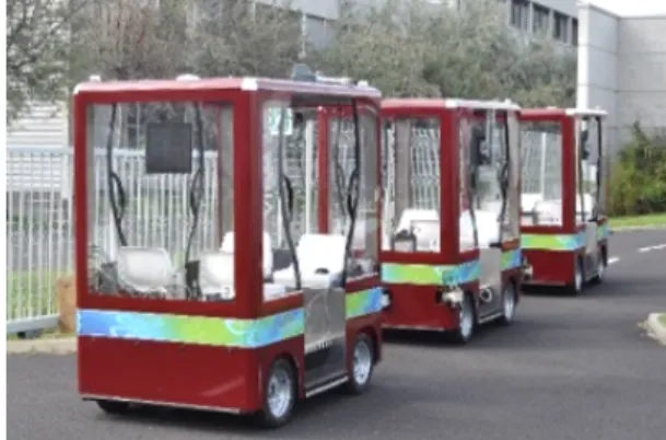
The numerical applications are done for the VIPALAB vehicles, which are autonomous electric vehicles for urban transportation (cf. Fig. 1).
The remainder of this paper will be organized as follows. Section II will give an overview on the works on autonomous vehicle control and will describe the pertinence and novelty of the proposed architecture. Section III will explain the design of the two blocks of the cascade control architecture. Section IV will show comparative simulations in a range situations for different controllers and architectures.
1 Institut Pascal, Universit´e Clermont Auvergne, Clermont-Ferrand,
2 Cranfield University, Cranfield, United Kingdom
Fig. 1. VIPALAB autonomous transport vehicles vehicles in a coordinated maneuver
II. TOWARDS A FLEXIBLE AND ROBUST CONTROL ARCHITECTURE A. Related works
The existing works on autonomous vehicle lateral control can be separated in two main categories. There are trajec-tory/target tracking algorithms on one side and yaw stabi-lization algorithms on the other side. Some approaches will be described as integrated and aim to fulfill those two tasks at the same time. For the tracking task, kinematic controllers are used in [14] and [3]. Depending on the implementation they can cover a range of speeds and situations but the lack of consideration of dynamic effects can be problematic for highly dynamic situations. Yaw stabilization (or active steering) schemes include [6] and [5] which use respectively the linear robust control framework and the MPC framework. Both approaches show very good performances, at the ex-pense of a robustness proof in [5] with the MPC design. As for integrated approaches, a first example based on a nonlinear kinematic controller is presented in [8]. Empirical terms have been added to a trajectory controller for dynamic effects compensation. In [7] is presented another integrated approach based on linear adaptive control. In [2] is presented an approach based on MPC. The choice of the technique mainly depends on the design objectives. Some other works cover the two tasks but with separate controllers for each one, which has the advantage to separate the objectives for each task and give an adapted answer. These approaches usually use two controllers in a cascade architecture. Such works for ground vehicles include [12] and [10]. Linear control is often used for the inner control loop. A similar cascade architecture for aerospace applications is presented in [4]. It is a common approach in Unmanned Aerial Vehicles (UAV)
design. Usually, these architectures fail to take into account the comfort, safety and implementability at the same time since they are more performance based. This is what the proposed design aims to do.
B. Architecture design
Compared to integrated design, the advantage of cas-cade architectures is the flexibility for multi-vehicle nav-igation and the natural separation between kinematic and dynamic phenomenons. Moreover, the trajectory tracking error dynamics are not on the same time scale than the car yaw dynamics. This separation is analoguous to the Guidance/Control framework [9] even though it is more a kinematic/dynamic separation.
The MPC has been used with great success to address trajectory tracking and yaw stabilization as an integrated approach. However it seems more relevant in this application to separate the yaw stabilization in a cascade architecture.
The inner loop for yaw stabilization has to deal with the uncertainty on the vehicle physical parameters. For instance the weight and inertia of the vehicle will undergo wide variations because of the variable passenger repartition. The friction coefficient µ will also be unknown and unmeasur-able.
For these reasons the linear robust control framework has been chosen to design the inner loop controller. It enables the robustness assessment of the controller under the model uncertainty, which is a big asset for ensuring safety.
The designed architecture is shown in Fig. 2. The MPC controller generates a desired yaw rate rdand a desired speed
vdto track the reference trajectory Xref. The inner controller
tracks the signal (rd, vd) by generating a desired steering
angle δd and acceleration ad to the vehicle. The state Xdyn
(resp. Xkin) is the dynamic (resp. kinematic) state of the
vehicle. It will be defined in section III-A (resp. III-B). III. PROPOSED CASCADE CONTROL
ARCHITECTURE
This architecture will have to fulfill the tasks of trajectory following as well as target tracking in order to be fit for multi-vehicle navigation. Trajectory following is the action of following a predefined line (defined in (x, y) coordinates) with a reference speed vref at each point. For target
follow-ing the same information is available but only at the current instant. More states can be known about the target, whether by sensing or communication. As mentioned in section II, the proposed architecture will have to handle the two tasks while ensuring passenger comfort and safety. The inner loop design will be described first and then the outer loop design, since it depends on the former.
A. Inner loop design
A mixed sensitivity H∞ controller has been chosen
be-cause it is an optimal design dechnique, and it has explicit disturbance rejection and frequency domain performance specifications. The disturbance rejection characteristics are interesting because it will dictate the vehicle’s behaviour
TABLE I
PARAMETER VALUES FOR UNCERTAIN CAR PLANT STUDY
parameter notation value
wheelbase lb 3m
inertial radius ir 1.5m
cornering stiffnesses cf, cr 700N/deg
actuator time constant τact 0.6s
mass m 600kg ± 30%
CG position to front axle lf 1.4m ± 20%
speed v 3m/s ± 50%
friction coefficient µ 0.65 ± 50%
under wind gusts. Too strong of a reaction could be seen as dangerous and uncomfortable.
For this application the model in the state space form is shown in (1). It is based on the kinematic bicycle representa-tion. It consists of a 2 degree of freedom (DoF) model for the sideslip β and yaw rate r dynamics and a first order model of time constant τact for the evolution of δ, the steering angle.
The overall state is Xdyn = (β, r, δ)T (resp. sideslip, yaw
rate and steering angle defined in Fig. 3). The input is the desired steering angle δd. This model has been presented in
depth in [1]. It is suitable for low speed situations such as urban traffic. ˙ Xdyn= a11 a12 b1 a21 a22 b2 0 0 −τact−1 Xdyn+ 0 0 τact−1 δd (1)
The coefficients aij and bi depend on the constants
cf, cr, m, v, J, lb, lf defined in Table I.
The following range of configurations has been consid-ered:
• from zero passenger to four passengers of 100kg each • speeds from 1.5m/s to 4.5m/s
• friction coeff in [0.3, 1] (from a slippery wet road to a dry road)
• Centre of Gravity (CoG) from 1.1m to 1.6m to front axle (because of the passenger repartition)
The corresponding uncertain variables have been summa-rized in Table I. As a way to reduce the number of uncertain variables, J has been considered proportional to m with the intermediate of the inertial radius ir (c.f. [1]).
The result of the H∞ design is shown in (2) with KCF
being the feedforward filter and KDR being the feedback
filter. The filters have been approximated by second order transfer functions to make the implementation faster.
KCF(s) = s2+ 21.2s + 158.2 s2+ 20s + 156.3 KDR(s) = 250(s + 124)(s + 1.67) s(s + 17.5) (2)
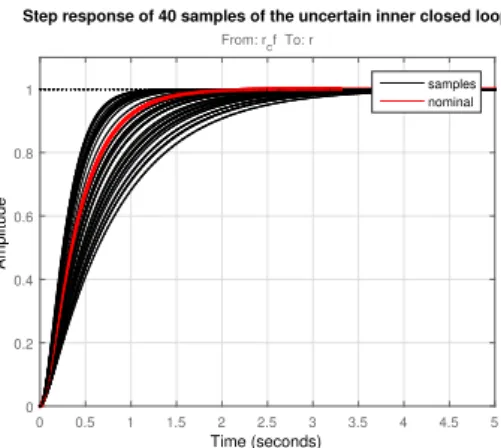
The robustness analysis shows that the design is robust to the modeled uncertainty. The performance analysis shows that the rise time for the yaw rate is always between 0.3s and 0.8s with a nominal value at 0.5s and the system is always well damped (as seen in Fig. 4).
Since the system is always well damped (there is no overshoot), it will be approximated by a first order system
Fig. 2. Designed cascade architecture
Fig. 3. Dynamic bicycle model conventions
0 0.5 1 1.5 2 2.5 3 3.5 4 4.5 5 0 0.2 0.4 0.6 0.8 1 From: rcf To: r samples nominal Step response of 40 samples of the uncertain inner closed loop
Time (seconds)
Amplitude
Fig. 4. Closed-loop step response envelope
in the following developments, making for a simpler model for the MPC.
B. Outer loop design
The outer loop controller (cf. Fig 2) needs to address the problem of stabilizing the vehicle around a moving target or a reference trajectory.
Even though it is a classical approach, MPC has good qualities to address our problem: it finds an optimal solution, can inherently deal with non linear processes such as car steering and can include constraints on the states and control signal (linked to comfort and safety). The prediction is also valuable to deal with slow dynamics and to anticipate future situations.
The main problem of MPC is that it always needs a reference trajectory over a finite horizon. In multi-vehicle navigation it is not always available and thus needs to be predicted to enable the use of MPC. Fig. 5 shows a situation where a reference trajectory for the virtual target T that VF
(the follower) has to follow is only partially known over the
MPC horizon. In this situation the aim is to keep constant offsets ∆yref and ∆sref with the trajectory of VL (the
leader). As the prediction horizon of the MPC depends on the model dynamics, it is not correlated to how far the target is to the leading vehicle. Thus a big MPC horizon and a small leader/target distance can lead to such a situation.
Fig. 5. Partial availability of a reference trajectory in leader/follower navigation
The reference trajectory prediction is based on the hy-potheses that the yaw rate r and speed v of the leader are constant. The states for the prediction are the same as the MPC presented later in (3). It generates a reference trajectory
ˆ
Xref(k + N |k) over the MPC prediction horizon N . The
MPC scheme can then be used seamlessly whether there is a reference trajectory over the whole prediction horizon or not and makes the architecture more flexible.
The chosen model for the MPC is shown in (3). At a timestep k, the state is Xkin(k) = (xk, yk, ψk, rk, vk)T
where xk, ykand ψk are defined in Fig. 6, rk is the yaw rate
of the car and vk its speed) and the input is U = (rd, vd)T
(the desired yaw rate and speed). The only parameters that describe the vehicle’s dynamics are τr and τv, the time
constants for the yaw rate and the speed responses which have been identified on the close inner loop (cf. Table II). The last parameter is the sampling time Tsof the loop. These
responses are assumed to be described by first order models. It is a realistic hypothesis as long as the real responses are well damped. This is the case here as seen in Fig. 4 thanks to the inner loop designed in section III-A.
xk+1 = xk+ Tsvkcos ψk yk+1 = yk+ Tsvksin ψk ψk+1 = ψk+ Tsrk rk+1 = rk+ τr−1(rd− rk) vk+1 = vk+ τv−1(vd− vk) (3)
The MPC scheme finds a control input Uopt that
mini-mizes a cost function J (U), where U = (Uk, ..., Uk+N) is
series of control signals to test over the prediction horizon N . This function is usually composed of a term that penalizes the errors to the reference trajectory and other terms to smooth the control signal.
Fig. 6. Navigation errors definition The penalized terms are:
• X, the matrix of differences w.r.t. the reference trajec-˜
tory over the prediction horizon N
• E(k + N |k) the navigation errors over the predictionˆ
horizon N. These errors are defined in Fig. 6 and further detailed in [14]. They are a convenient way to work in a local frame that is in the vehicle’s orientation.
• U the difference between the test input signal and the˜
previous optimal input signal
• U∆the differences between two successive input values
in the tested input signal (a.k.a. control effort)
The chosen cost function is defined in (4). It is a weighted sum of the penalty terms:
J (U) = ˜XTQ ˜X + ˆE(k + N |k)TS ˆE(k + N |k) + ˜UTR ˜U + UT∆R∆U∆ (4)
The penalties on ˜U and U∆ tend to smooth the tracking
and are often encountered in nonlinear MPC schemes. The penalty on the navigation errors allows to separately penalize the lateral and longitudinal errors (exand ey) and have been
preferred to the penalty on the state difference ˜X. The values of the weight matrices Q, S, R and R∆ are compiled in
Table II. The raw state difference ˜X has not been penalized except for the speed difference, which was found to smooth the longitudinal tracking.
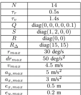
For comfort and safety, the following constraints have been introduced: • |rd| ≤ rmax • | ˙rd| ≤ drmax • vmin≤ vd ≤ vmax • |ay,d| = |vdrd| ≤ ay,max • |ax,d| = ∆vd/Ts≤ ax,max • |κd| = |rd/vd| ≤ κmax TABLE II MPCCONTROLLER PARAMETERS N 14 τr 0.5s τv 1.4s Q diag(0, 0, 0, 0, 0.1) S diag(1, 2, 0, 0) R diag(0, 0) R∆ diag(15, 15) rmax 30 deg/s drmax 50 deg/s2 vmax 4.5 m/s ay,max 5 m/s2 ax,max 3 m/s2 ex,max 0.5 m ey,max 0.2 m
The constraints on the yaw rate rd, the yaw rate derivative
˙rd and the lateral/longitudinal accelerations ay,d and ax,d
are here for comfort. The constraints on the speed vd and
the curvature κd are physical limitations of the vehicle. Two
additional constraints on the tracking errors have been added: |ex| ≤ ex,max and |ey| ≤ ey,max. These constraints are used
to ensure the vehicle will stay within given bounds around the target. For example, the constraint on ey will depend on
the road width. The numerical values used for the constraints are compiled in Table II. The optimization function used for the simulations is the fmincon Matlab optimization function under constraints. The input constraints will always be re-spected (it restricts the search space) and the function will try to find a solution that respects the additional constraints on the tracking errors, unless impossible. In the latter case, the optimization function’s output will mention that the constraints were not respected. This information can be used to prevent the violation of constraints before it actually happens. Finally, the MPC scheme runs approximately in 20 seconds for a 10 seconds Simulink simulation with a modern computer (a 2013 Intel i5 equipped laptop) and a loop rate of 10Hz.
C. Conclusion
The proposed architecture is comprised of two loops in cascade that aim to solve the trajectory tracking/target following problems under comfort and safety constraints. The task separation allows to split the constraints and to focus on different aspects of the problem at each stage as well as allowing a simpler design overall.
IV. SIMULATIONS AND RESULTS A. Model Used
The model used for the simulations consists of a 3DoF bicycle chassis model with a linear tyre model (for both the longitudinal and lateral forces). The simulations have been performed in Simulink.
The model for the simulations is based on the one pre-sented in section III-A. The rotational wheel dynamics have been added in order to have a realistic longitudinal behaviour. Thus the state vector is defined as X = (β, r, v, ωf, ωr)T
ωr) is the front (resp. rear) wheel rotational speed. The
input vector is U = (δd, ad)T, the desired steering angle
and longitudinal acceleration. These inputs are transformed into actual wheel angle and acceleration by the {actuator + controller} systems modeled by first order transfer functions of time constant 0.6s (resp 1s) and damping 0.8. The front and rear axles inertias are Jf = Jr= 0.45kg.m−2 and the
longitudinal tyre stiffnesses are Cl,f = Cl,r = 1e4N. The
other model parameters will be within the range of values used for controller design (cf. Table I). Unless specified otherwise, the nominal values have been taken.
B. Simulation scenarios
Comparisons will be made with two kinematic controllers. The first controller is the one presented in [14] and [13]. For simplicity it will be referenced as the ”Vilca” controller. It is a nonlinear control law designed for both dynamic target following and waypoint navigation. It is based on a Lyapunov function design and is a recent example of a flexible kinematic controller. The other one is the ”Pure Pur-suit” controller [11], a widely used kinematic controller for trajectory tracking because of its simplicity and efficiency. It is a non linear controller that computes a curvature to reach a point on the trajectory at a look-ahead distance. This distance is usually proportional to the vehcile speed with a coefficient kP P within a lower and upper bound (cf. Table III). Both
algorithms compute the steering angle corresponding to the desired curvature under kinematic hypotheses, thus not taking into account actuator delays and slip.
For the simulations, the virtual target follows a sinusoidal path at a constant speed (cf. Fig 7). For the MPC controller it is assumed that no information of the target’s future path is available to put it in difficult conditions. As a consequence, the prediction module described in section III-B will be used. It is on the other hand assumed that the trajectory is entirely available when using the pursuit controller, thus giving it more favorable conditions.
Two test case are presented:
• Behaviour comparison: A test at low speed to compare the behavior of the three controllers. For this test the nominal values for the car model will mostly be used.
• Safety and comfort assessment: A test at a higher speed and non-nominal car model values to check the robustness of the approaches. This test will also serve to check if the comfort constraints with our approach are respected in more agressive maneuvers.
The common (resp. variable) parameters for the simulation scenarios are compiled in Table III (resp. Table IV-B). C. Behaviour comparison
All the nominal parameters for the model have been taken except the speed which is 2m/s. The MPC shows a very good tracking compared to the two other methods (cf Fig. 8). However the control signals (Fig. 9) and the comfort indicators (Fig. 10) are approximately of the same magnitude for the three approaches. In easy maneuvers like this one the proposed architecture behaves well but has an edge on
TABLE III
COMMON SIMULATIONS PARAMETERS
parameter value
initial vehicle position (1, 1) (m)
initial vehicle heading 30◦
target path curvature variation rate 0.1 Hz
max target path curvature 1/15m−1
Vilca’s law coefficients KV (1, 2.2, 8, 0.1, 0.01, 0.6)
Pursuit law look-ahead coeff. kP P 0.5
Pursuit law look-ahead dist. bounds [1, 5] (m)
outer loop sampling time Ts,g 1/10s
inner loop sampling time Ts,c 1/50s
TABLE IV
VARIABLE SIMULATION PARAMETERS
parameter value
First simulation Second simulation initial target position (1.5, 1.5) (m) (2, 2) (m)
initial target heading 30◦ 40◦
Target speed 2m/s 4m/s
vehicle mass 600kg 750kg
friction coefficient µ 0.65 0.4
neither the pursuit controller or on Vilca’s controller in terms of comfort.
D. Safety and comfort assessment
In this simulation, the safety has been assessed by check-ing the trackcheck-ing performance under a change of mass, friction coefficient and speed. The respect of the comfort constraints with the proposed cascade architecture has been tested and compared with the behaviour of the other controllers. In this series, the target initial position was further from the vehicle initial position (cf. Table IV-B) to study the behaviour of the controllers when a more agressive maneuver is required to follow the target.
The tracking performance of the designed cascade archi-tecture is now far better than both the Pursuit controller and Vilca’s controller (cf. Fig. 11). The latter one shows an unstable oscillatory behaviour at these higher speeds because it neither anticipates the trajectory nor the actuator delay. The performance of the cascade architecture also shows the
x (m) 0 2 4 6 8 10 12 14 16 18 20 y (m) 0 2 4 6 8 10 12
14 path of target and vehicle
target PP Vilca Cascade
t (s) 0 1 2 3 4 5 6 7 8 9 10 ex (m) -1 -0.5 0 0.5 1 error e x PP Vilca Cascade t (s) 0 1 2 3 4 5 6 7 8 9 10 ey (m) -0.5 0 0.5 error e y PP Vilca Cascade
Fig. 8. Tracking performance (1stseries)
t (s) 0 1 2 3 4 5 6 7 8 9 10 vcar (m/s 2) 1 2 3 4 5 desired speed PP Vilca Cascade t (s) 0 1 2 3 4 5 6 7 8 9 10 rd (m -1) -0.5 0 0.5
desired yaw rate
PP Vilca Cascade
Fig. 9. Control signals (1stseries)
t (s) 0 1 2 3 4 5 6 7 8 9 10 rcar (m -1) -0.5 0 0.5
measured yaw rate
PP Vilca Cascade t (s) 0 1 2 3 4 5 6 7 8 9 10 ay,CG (m.s -2) -5 0 5
measured lateral acceleration at CG
PP Vilca Cascade
Fig. 10. Comfort indicators (1stseries)
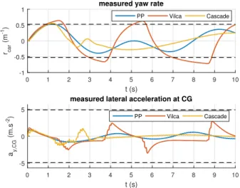
effectiveness of the inner controller to stabilize the yaw dynamics with a non nominal model. The control signals (Fig. 12) show an effective capping of both the desired speed and yaw rate with the cascade architecture, leading to a faster tracking errors convergence while respecting the introduced constraints. The comfort indicators (cf. Fig. 13) show undamped oscillations for both the Pursuit and Vilca’s controller, and a slight overshoot for the cascade design. It could be removed with finer tuning of the MPC controller or the use of the real target’s trajectory information.
t (s) 0 1 2 3 4 5 6 7 8 9 10 ex (m) -2 -1 0 1 2 error e x PP Vilca Cascade t (s) 0 1 2 3 4 5 6 7 8 9 10 ey (m) -1 -0.5 0 0.5 1 error e y PP Vilca Cascade
Fig. 11. Tracking performance (2ndseries)
t (s) 0 1 2 3 4 5 6 7 8 9 10 vcar (m/s 2) 1 2 3 4 5 desired speed PP Vilca Cascade t (s) 0 1 2 3 4 5 6 7 8 9 10 rd (m -1) -1 -0.5 0 0.5
1 desired yaw rate
Fig. 12. Control signals (1stseries)
V. CONCLUSIONS
In this paper has been proposed a cascade architecture for autonomous vehicle navigation. This architecture seamlessly fills the tasks of trajectory/path tracking as well as dynamic target following and thus can cope with multi-vehicle sce-narios. The architecture is divided into a robust low-level yaw stabilization controller that focuses on the vehicle’s dynamics and a high-level tracking MPC controller that
t (s) 0 1 2 3 4 5 6 7 8 9 10 rcar (m -1) -1 -0.5 0 0.5
1 measured yaw rate
PP Vilca Cascade t (s) 0 1 2 3 4 5 6 7 8 9 10 ay,CG (m.s -2) -5 0 5
measured lateral acceleration at CG
PP Vilca Cascade
Fig. 13. Comfort indicators (2ndseries)
focuses mainly on the kinematics. This architecture shows an improvement in tracking performances, safety and flexi-bility compared to usual kinematic controllers for trajectory tracking. It is not intended to have an edge on performances compared to integrated approaches for trajectory tracking but to improve robustness and implementability. Further work will be carried out to check the performances of a linear MPC controller as well as a robustification of the MPC scheme. Real time implementability will be evaluated and Linear Parameter Varying (LPV) techniques for the low-level controller (parametrized by speed) will be investigated to improve its performance and operational envelope.
ACKNOWLEDGMENT
This work has been sponsored by the French government research program Investissements d’avenir through the Robo-tEx Equipment of Excellence (ANR-10-EQPX-44) and the IMoBS3 Laboratory of Excellence (ANR-10-LABX-16-01), by the European Union through the program Regional com-petitiveness and employment 2014-2020 (FEDER - AURA region) and by the AURA region.
REFERENCES
[1] J¨urgen Ackermann. Robust Control for Car Steering. Tech. rep. German Aerospace Center, Institute of Robotics and System Dynamics, 1999.
[2] Pedro Aguiar, Andrea Alessandretti, and Colin N Jones. “Trajectory-tracking and path-following con-trollers for constrained underactuated vehicles using Model Predictive Control”. In: European Control Con-ference(2013), pp. 1371–1376.
[3] A. Broggi et al. Autonomous vehicles control in the VisLab Intercontinental Autonomous Challenge. 2012. [4] Dongkyoung Chwa and Jin Young Choi. “Adaptive Nonlinear Guidance Law Considering Control Loop Dynamics”. In: IEEE Transactions on Aerospace and Electronic Systems39.4 (2003), pp. 1134–1143.
[5] Paolo Falcone and Francesco Borrelli. “Low com-plexity MPC schemes for integrated vehicle dynamics control problems”. In: International Symposium on Advanced Vehicle Control1 (2008), pp. 875–880. [6] Simon Hecker. “Robust Hinf-based vehicle steering
control design”. In: Computer Aided Control System Design, 2006 IEEE International Conference on Con-trol Applications, 2006 IEEE International Symposium on Intelligent Control, 2006 IEEE. IEEE, Oct. 2006, pp. 1294–1299.
[7] Pushkar Hingwe et al. “Linear parameter varying controller for automated lane guidance: Experimen-tal study on tractor-trailers”. In: IEEE Transactions on Control Systems Technology 10.6 (Nov. 2002), pp. 793–806.
[8] Gabriel M. Hoffmann et al. “Autonomous Automo-bile Trajectory Tracking for Off-Road Driving : Con-troller Design , Experimental Validation and Racing”. In: Proceedings of the American Control Conference (2007), pp. 2296–2301.
[9] Farid Kendoul. “Survey of advances in guidance, navigation, and control of unmanned rotorcraft sys-tems”. In: Journal of Field Robotics 29.2 (Mar. 2012), pp. 315–378. arXiv: 10.1.1.91.5767.
[10] Alexey S. Matveev, Hamid Teimoori, and Andrey V. Savkin. “A method for guidance and control of an autonomous vehicle in problems of border patrolling and obstacle avoidance”. In: Automatica 47.3 (2011), pp. 515–524.
[11] Jes´us Morales et al. “Pure-pursuit reactive path track-ing for nonholonomic mobile robots with a 2D laser scanner”. In: Eurasip Journal on Advances in Signal Processing2009.1 (2009), p. 935237.
[12] Joshu´e P´erez, Vicente Milan´es, and Enrique Onieva. “Cascade architecture for lateral control in au-tonomous vehicles”. In: IEEE Transactions on In-telligent Transportation Systems 12.1 (Mar. 2011), pp. 73–82.
[13] Jos´e Miguel Vilca, Lounis Adouane, and Youcef Mezouar. “A novel safe and flexible control strategy based on target reaching for the navigation of urban vehicles”. In: Robotics and Autonomous Systems 70 (Aug. 2015), pp. 215–226.
[14] Jos´e Miguel Vilca, Lounis Adouane, and Youcef Mezouar. “An Overall Control Strategy Based on Tar-get Reaching for the Navigation of an Urban Electric Vehicle”. In: International Conference on Intelligent Robots and Systems (IROS)(2013), pp. 728–734. [15] Danny Yadron and Dan Tynan. “Tesla driver dies in
first fatal crash while using autopilot mode”. In: The Guardian(2016).