HAL Id: halshs-00564683
https://halshs.archives-ouvertes.fr/halshs-00564683
Preprint submitted on 9 Feb 2011
HAL is a multi-disciplinary open access archive for the deposit and dissemination of sci-entific research documents, whether they are pub-lished or not. The documents may come from teaching and research institutions in France or abroad, or from public or private research centers.
L’archive ouverte pluridisciplinaire HAL, est destinée au dépôt et à la diffusion de documents scientifiques de niveau recherche, publiés ou non, émanant des établissements d’enseignement et de recherche français ou étrangers, des laboratoires publics ou privés.
Growth
Jean-Louis Arcand, Marcel Dagenais
To cite this version:
Jean-Louis Arcand, Marcel Dagenais. Errors in Variables and the Empirics of Economic Growth. 2011. �halshs-00564683�
of Economic Growth
Jean-Louis Arcandy Marcel Dagenaisz
November 25, 2005
Abstract
We examine cross-sectional empirical evidence on the determinants of economic growth in light of an instrumental variables estimator, based on sample moments of order higher than two, which does not require extraneous instruments and which remains consistent, under quite reasonable assumptions, when measurement errors a¤ect the explanatory variables. We focus on several in‡uential papers — Barro (1991), Mankiw, Romer, and Weil (1992), Sachs and Warner (1997a), Easterly and Levine (1997), Levine and Zervos (1998)— and …nd that many of their results are “fragile”. We argue that the application of our estimator to cross-sectional empirical studies of the determinants of growth yields important insights which may qualify previous …ndings in the literature, especially given the errors in variables problems which are known to plague commonly used cross-sectional datasets.
Keywords: errors in variables, economic growth JEL: C52, C21, O41
1
Introduction
1.1 Motivation
In two celebrated articles, Barro (1991) (henceforth, Barro) and Mankiw, Romer, and Weil (1992) (henceforth, MRW) provided in‡uential empirical contributions that largely shaped the stylized facts accepted by most economists as to the determinants of economic growth. In another contribution, Sachs and Warner (1997a) and Sachs and Warner (1997b) (henceforth, SW) provided widely cited evidence on the fundamental factors that determine growth as well as the sources of slow growth in the economies of sub-saharan Africa. This paper considers whether the results reported by Barro, MRW and SW, as well as two other in‡uential papers –Easterly and Levine (1997) (henceforth, EL), and Levine and Zervos (1998) (henceforth, LZ)–
We acknowledge the …nancial support of the PARADI project, funded by a grant from the Canadian Interna-tional Development Agency (CIDA). We also wish to thank numerous seminar participants and an anonymous referee. The usual disclaimer applies.
yCERDI-CNRS, Université d’Auvergne and European Development Network (EUDN). 65 boulevard François
Mitterrand, 63000, Clermont Ferrand, France. Email: arcandjl@alum.mit.edu.
zMarcel Dagenais died on 14 February, 2001. This paper is dedicated to his memory. He was professor of
economics at the Université de Montréal. He is sorely missed by all those who knew him and had the good fortune to be touched by his rare combination of joie de vivre and analytical rigour.
are signi…cantly a¤ected by an error in variables problem, and whether correcting for this problem changes our perception of the forces driving economic growth.
These papers touch on or explicitly test many of the fundamental questions associated with the empirics of long-run economic growth, including: conditional convergence (all of the papers), the role of government (Barro), the human capital augmented Solow model (MRW), geography (SW), ethnolinguistic fragmentation as an explanation for low growth in sub-saharan Africa (EL and SW), and stock markets and banking (LZ). While this list of growth topics is far from being exhaustive, we would argue that it constitutes a fairly representative sample of the issues that have occupied growth empiricists over the past decade and a half.
1.2 The problem and a potential solution
Despite the care which was put into the construction of the data used in these papers, it is widely believed that cross-sectional international data are plagued by errors in variables (EV). Srinivasan (1994), for example, does not mince his words: “The disturbing conclusion emerg-ing... is that the situation with respect to the quality, coverage, intertemporal and international comparability of published data on vital aspects of the development process is still abysmal in spite of decades of e¤orts at improvements.”1
If the regressors included in commonly estimated growth rate or per capita GDP equations di¤er from the “true” regressors because of EV, then the regression error structure does not satisfy the usual Gauss-Markov conditions and the estimated parameters will be inconsistent.2 In this paper we reconsider widely-publicized cross-sectional results in the economic growth literature in the light of the “higher moments”instrumental variables (IV) estimator, developed by Dagenais and Dagenais (1997), which is robust, under quite reasonable assumptions, to EV. We test the null-hypothesis of the absence of EV using a Hausman-type test, and assess the validity of our proposed IVs using both the standard Sargan test of the overidentifying restrictions and a recent instrument validity test proposed by Hahn and Hausman (2002a).
1.3 Is it worth the trouble?
While properly accounting for EV in empirical growth regressions is interesting from the econo-metric perspective, the empirically-minded reader will be wondering out loud “so what?”After all, the proof of the pudding is in the eating: does the estimator we propose yield results which di¤er substantially enough from the OLS results to warrant its use in practice? Do our results change one’s understanding of the empirics of economic growth? If the answer is “no,”then we have merely uncovered an empirical “fact”(the presence of EV in less developed country (LDC) national income accounting data) which was already well-known, and our econometric artillery
1
p. 23-24. In the context of his review of empirical studies of the e¤ects of trade policy orientation on growth, Edwards (1993) (p. 1390) notes that “in order to gain further insights into these issues, it is fundamental to adopt econometric methodologies that deal speci…cally with errors in variables, that investigate formally the robustness of speci…c results, and that rely systematically on sensitivity analysis... from an econometric perspective, one of the most serious shortcomings of the cross-section papers discussed [in his survey]... is the lack of e¤orts to implement in a systematic way a battery of tests that deal with the degree of robustness (or fragility) of the results.”
2
Nelson (1995) consider the classic case of attenuation bias of OLS estimates when several variables are a¤ected by measurement error.
is merely overkill. If the answer is "yes", then the problem of EV is su¢ ciently important to merit its careful consideration in formulating and testing hypotheses regarding the determinants of economic growth.
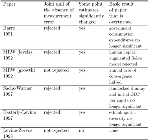
Unsurprisingly, our answer to the above questions is “yes.” We argue that many of our results using the higher moments estimator are su¢ ciently di¤erent from those in the papers we consider to warrant (i) more careful scrutiny of the cross-sectional data and (ii) the application of our estimator in preference to OLS. Our results suggest that several of the conclusions regarding the empirics of economic growth drawn by the papers considered here may not be as strong as they may appear. Table 1 concisely summarizes our main empirical …ndings.
1.4 Errors in variables versus speci…cation error
We are not alone in subjecting a sample of empirical results from the large cross-sectional growth literature to some form of test for their robustness. For example, Levine and Renelt (1992) use Leamer’s extreme bounds analysis to show that almost all variables included in a plethora of commonly estimated cross-country growth rate regressions are not robust to variations in the set of explanatory variables. Their analysis can be interpreted as a test of the underlying structural model used to justify the inclusion or exclusion of certain variables from the estimated relationship. Another example is furnished by Temple (1998) who considers the robustness of the MRW results to classical EV using the Klepper and Leamer (1984) reverse regression technique as well as classical method of moments estimators.
As in Temple, the analysis in this paper does not explicitly question the validity of the underlying model but focuses on the properties of the regressors included in the estimated equation. Of course, since growth equations may su¤er from speci…cation error, and since the test procedure we use can be interpreted as a variant on the well-known Hausman instrumental variables (IV) speci…cation test, it is likely that a portion of what we ascribe to EV can be attributed to errors in speci…cation. The empirical researcher in search of a means of testing the robustness of her results is therefore left with the following choice : (i) the use of Leamer’s extreme bounds analysis if EV may be considered relatively unimportant and the major concern is the speci…cation of the estimated equation, (ii) the use of our estimator if the validity of the speci…cation is less in doubt than is the "purity" of the underlying data. Keeping this last caveat in mind, it would seem to be of considerable interest to subject empirical results such as those considered here to a test for the presence of EV.
2
The Estimator and the test for errors in variables
2.1 The econometric problem and previous solutions using higher moments
The data employed in most growth regressions is almost certainly subject to EV. Since even aggregate time series for industrialized countries are, according to Morgenstern (1963), Lan-gaskens and Van Rickeghem (1974) and Lipsey and Tice (1989), subject to important EV, a fortiori one would expect this problem to plague a broad cross-section of data from 100 di¤erent countries, many of them LDCs where national income accounting practice is sketchy at best.
The standard response of the econometrician to an EV problem is of course to resort to IV techniques in order to obtain consistent parameter estimates.
The problems with this approach in the context of cross-sectional growth regressions are that (i) some of the potential excluded instruments may in fact be correlated with the regression errors and should probably be included themselves as endogenous variables in a more complete simultaneous structural form, leading to the need for additional (unavailable) exogenous instru-ments, (ii) eligible instruments may simply not be available for a broad enough cross section of countries to permit the use of IV techniques, and (iii) it may not be feasible to verify that the proposed instruments satisfy the desired orthogonality assumptions because of the absence of overidenti…cation.
Given the three points raised above, this paper proposes an alternative to standard IV techniques that has received no attention in the empirical growth literature: the use of consistent estimators based on sample moments of order higher than two. There are a number of such estimators available. Estimators based on third-order sample moments have been proposed by Geary (1942), Drion (1951) and Pal (1980), while Geary (1942) and Pal (1980) also propose estimators based on fourth-order cumulants.
The problem with these estimators, however, is that their behavior is substantially more erratic than the corresponding least squares estimators (see, e.g., Kendall and Stuart (1963), Malinvaud (1978)). One possible solution to this endemic instability, which is adopted in this paper, is to use a higher moments estimator suggested by Dagenais and Dagenais (1997) which is essentially a linear matrix-weighted combination of third and fourth moment estimators. As pointed out by Pal (1980), all higher moments estimators can be considered as a special type of IV estimators where the instruments are given by functions of the original variables raised to some power.
2.2 The estimator
2.2.1 Basic notation
The typical growth regression can be written in matrix notation as
y1 =ye2 + u; (1)
where ey2 is an N r matrix of exogenous explanatory variables measured without error, with
empirical distribution such that p limey20ey2
N = Q, where Q is a …nite non-singular matrix, N is
sample size, and where y1 is the N 1 vector of observations of the dependent variable. For
notational convenience, equation (1) corresponds to the growth regression in which all variables known ex ante to be measured without error (such as the intercept term or continent dummies) have been "partialled out" of the speci…cation. The N 1 vector u is assumed to be distributed N (0; 2uIN). The r 1 vector and 2u are unknown parameters. The problem of EV is posed
econometrically by assuming thatye2 is unobservable and that instead one observes the matrix
y2, where
and V is an N r matrix of normally distributed errors in the variables. Furthermore, we assume that V ar [V ec(V )] = IN where V ar [:] stands for the covariance matrix and where
is an r r symmetric positive de…nite matrix. This assumption implies that (i) the errors in the variables are independent between observations, but (ii) not between variables.
2.2.2 Discussion of the underlying assumptions
In the context of a set of regressors based on a heterogeneous group of approximately 100 di¤erent countries, both these assumptions appear to be reasonable as a …rst approximation. Indeed, there is no reason to believe that errors in the statistical procedures used to measure, say, investment, are signi…cantly correlated across countries (this is particularly true given the great heterogeneity in the standard of accounting practices among LDCs and DCs), although problems might arise within subsets of countries which follow similar accounting procedures. Without studying the national income accounting procedures of all countries in the sample, however, this assumption appears reasonable, prima facie.3
Second, there is good reason to believe that an LDC where the measurement of one macro-economic aggregate is subject to error will also display similar lacunae in the measurement of other series. Finally, the assumption also implies that, for a given variable, the errors in mea-surement are homoskedastic. This assumption may not be so reasonable if one believes either that the accuracy of the data is an increasing function of the level of development, or that the accuracy of the data is correlated with an unknown set of variables (which may include some of the regressors). In the …rst case, a correction based speci…cally on the hypothesized relationship between the magnitude of the EV and the explanatory variable in question is called for. In the second case a correction for heteroskedasticity of unknown form (e.g., White (1980)) might seem to be appropriate.4
2.2.3 The proposed instrument set
Given the above considerations, it seems most appropriate to use a regression estimator which remains consistent in the presence of EV. The estimator used here is one of the estimators suggested by Dagenais and Dagenais (1997), where the matrix of feasible instruments, denoted
3
The assumption may be not be quite so ino¤ensive when using Heston-Summers data since the authors extend their data to all "non-benchmark" countries using the same method. This may result in some degree of correlation between countries. Note however that our "higher moment estimator" does remain consistent when measurement errors are correlated between observations. Its asymptotic covariance matrix, however, would be di¤erent.
4
The second problem was addressed in the empirical work underlying this paper through the use of Huber-White standard errors. The changes in statistical inference that resulted were not su¢ ciently important to warrant their inclusion in the results presented below.
by Z = (z1; z2; z3; z4; z5; z6; z7), is given by: z1 = y2 y2; z2 = y2 y1; z3 = y1 y1; z4 = y2 y2 y2 3y2 y02y2 N Ir ; z5 = y2 y2 y1 2y2 y02y1 N Ir y1 0 r y02y1 N Ir ; z6 = y2 y1 y1 y2 y0 1y1 N y1 y0 1y2 N ; z7 = y1 y1 y1 3y1 y01y1 N ;
and where the symbol designates the Hadamard element-by-element matrix multiplication operator, Iris an r-dimensional identity matrix, and ris an r 1 vector of ones. Detailed proofs
of the orthogonality of these instruments with respect to the disturbance term are provided in Dagenais and Dagenais (1997).
The proposed estimator is a Fuller (1977) modi…ed IV estimator, with the "Fuller constant" set equal to 1. This estimator possesses …nite moments for all values of the "concentration pa-rameter" associated with the reduced forms, as well as good small sample properties. Moreover, Hahn, Hausman, and Kuersteiner (2004) have provided extensive Montecarlo experiment results that show that this estimator performs well when compared to other prominent IV estimators, under weak instruments, an issue we shall address below.
The resulting "higher moments" estimator, which we shall denote by H, is consistent when there are EV and is also much less erratic than other estimators based on sample moments of order higher than two heretofore suggested in the literature.5 Details concerning the con-struction of the Fuller estimator based on these instruments, as well as the variance-covariance matrix, are provided in Dagenais and Dagenais (1997).
2.2.4 Testing for errors in variables
The test for the presence of EV that we apply is a Hausman (1978) test. This asymptotic test is most easily performed by the following procedure. First, run the augmented regression by OLS:
y1= y2 + ^w H + " (3)
where ^w = y2 PZy2, PZ = Z(Z0Z) 1Z0; H is a vector of parameters and " is the vector of
the regression errors. Second, test H = 0 using the usual F -test.
If there are no errors in the variables, y2 =ye2 and y1 = y2 + u. Therefore under the null
hypothesis of no errors in the variables, " = u and H = 0.
5
Note that other implementations of the proposed instrument set are possible, apart from the Fuller-estimator chosen here. These include GMM (the road taken in an earlier paper by Dagenais and Dagenais (1994)), Nagar (or bias-adjusted 2SLS, see Donald and Newey (2001)), or general k-class estimation. The Hahn and Hausman (2002a) tests used in this paper are based on using the proposed instrument set in the context of the Nagar estimator.
In what follows, we will also apply the equivalent t-test to each individual right-hand-side (RHS) variable so as to attempt to isolate the source of any existing EV-induced bias. From equation (3), it is readily seen that the power of the test that any given element of H is equal to zero and hence that the associated variable has no EV, will depend in part on the collinearity between the columns of the ^! matrix. As for any other statistical test, a low p-value associated with an individual element of H may lead one to reject the null of the absence of EV in the corresponding variable with a certain degree of con…dence; but a high p-value may not indicate its absence. It may stem simply from a lack of power of the test, due for example to a problem of collinearity. Furthermore, as for any other test, the validity of our test is conditional on the fact that the model is correctly speci…ed.
2.2.5 Montecarlo evidence on the performance of the estimator
Since, in Dagenais and Dagenais (1997), the reported Monte Carlo experiments were performed on samples of 700 observations or more, additional experiments were carried out on smaller samples, with data exhibiting the same characteristics as those used in the papers under con-sideration here. In what follows, we present Montecarlo experiments based on the MRW dataset.
We began by running a regression of the level of GDP per capita in 1985 on a constant, the population growth rate, the investment ratio and the enrollment rate (all variables are in logs), using the 98 observations in the MRW dataset. Variables were then scaled so that the intercept and all coe¢ cients were equal to 1. We then used these scaled variables to generate levels of the dependent variable according to:
y1= 1 +ey2+ye3+ey4+ u;
where u is the normal regression error term. Normal random errors were then added to e
y3 so as to yield y3 =ye3+ V , and the variance of u was set so as to ensure an R 2
of 0.778, which corresponds to the empirical value in the baseline MRW regression. As in the original Montecarlo experiments presented in Dagenais and Dagenais (1997), the ratio of the variance of measurement errors V to the variance of ye3 was initially set equal to 0.3. In experiment
1, we instrumented all variables using Z, whereas in experiment 2, only y3 was assumed to be
subject to EV, with ey2 and ey4 serving as their own instruments.
The main results that emerge from Montecarlo experiments 1 and 2, reported in Table 2, when one instruments using Z = (z1; z4), are the following. First, bias is substantially smaller
for H than for OLS. Second, Root Mean-Squared Error (RMSE) is generally higher for H than for OLS, though the RMSE can be reduced for the H estimator if one limits the number of variables assumed to be measured with error. Third, the size of type I errors are extremely high for OLS, with respect to the theoretical value of 5%, whereas the corresponding …gures are quite close to the true value for H.6 Fourth, the power of the joint EV test is quite low
with the sample size considered here (this is in contrast to the larger sample sizes considered
6
The sizes of the type I errors were computed as the percentage of replications for which the true value of the parameter was not included within the 95% con…dence interval.
in Dagenais and Dagenais (1997)). From the empirical perspective, this implies, if one rejects the null of the absence of EV, that there is a strong presumption that they are present.
As with the Montecarlo experiments reported in Dagenais and Dagenais (1997), the estima-tor based on the full set of instruments (z1 through z7) performs less well than the estimator
based on z1 and z4 alone. This is true in terms of bias, RMSE and the size of type I errors.
The power of the joint EV tests is the same for both estimators.7 For all of these reasons, we shall present empirical results based on instrumenting with z1 and z4 alone.
In experiment 3, we set the coe¢ cient onye4 equal to zero. The correlation betweeney3 and
e
y4 in the results presented in Table 3 is equal to 0.633, and we increase the relative magnitude
of the variance of V , from 0.3 to 0.8. Despite the fact that ye4 was not a¤ected by an EV
problem, and that, in a simple regression asymptotic bias disappears when the coe¢ cient in question is equal to zero, the bias of the OLS estimate of 4 was substantial (0.204). Most importantly, the size of the type I error associated with the test that 4 = 0 was large (0.398), indicating that a t-test, based on a 95% con…dence level of the null that 4 = 0, would have been incorrectly rejected almost 40% of the time. Tu put it another way: in the Montecarlo experiment corresponding to Table 3, the OLS estimate of 4 was equal to 0.204, with an associated t-statistic of 1.747 (p-value = 0.081), whereas the higher moments estimate of 4 was 0.073, with a t-statistic of 0.266 (p-value = 0.790).
In the context of the cross-sectional data used in the papers considered here, where the explanatory variables are often highly correlated and the magnitude of EV on at least some variables is likely to be large, this experiment reveals that it is quite easy for one to conclude that a given variable is statistically signi…cant using OLS, when in fact its statistical signi…cance is spurious and stems from an EV problem a¤ecting another variable.
2.3 Instrument admissibility and instrument choice
A potential concern with the use of higher moments of the explanatory variables themselves as excluded instruments is that they may su¤er from a "weak instruments" problem, an issue that has come to the forefront of the econometrics literature in recent years. As is by now well known, weak instruments can lead to bias in IV estimation, and this bias does not vanish even with large sample sizes.8 Note that a …rst test of the underlying orthogonality conditions will be provided by the usual Sargan test of the overidentifying restrictions, although a more recent and robust diagnostic test of instrument validity will also be used, given that the Sargan test is known to possess poor size properties.
2.3.1 The Hahn-Hausman test
A recent procedure proposed by Hahn and Hausman (2002a) provides a joint test of instru-ment orthogonality and instruinstru-ment relevance (i.e. their "strength"). In terms of instrument
7Interestingly, the bias that emerges using z
1 through z7, when there is only one variable assumed to be
measured with error, takes on almost exactly the same value as that for OLS, suggesting that a situation of weak instruments is present (it is well-known that IV is biased towards OLS when the concentration parameter is near zero).
8
The standard discussion is provided by Bound, Jaeger, and Baker (1995). See also the excellent surveys by Stock, Wright, and Yogo (2002) and Hahn and Hausman (2003), and a recent very short primer on the ensuing biases by Hahn and Hausman (2002b).
relevance, and in contrast to the by-now standard Shea (1997) partial R2 and F statistics diagnostics on the reduced forms, which are based on the null hypothesis of weak instruments, Hahn and Hausman base their procedure on the null of strong instruments.
Consider the Bias-adjusted 2SLS estimator (B2SLS), which is an example of a k-class esti-mator, of which conventional 2SLS, Limited Information Maximum Likelihood (LIML) and the Fuller estimator are special cases. As an illustration, consider the particularly simple situation in which y2 is a scalar (i.e. r = 1). Then the k-class instrumental variables estimator for is
de…ned by bB2SLS = y02PZy1 y20MZy1 y0 2PZy2 y20MZy2 ;
where MZ = IK PZ is the orthogonal complement to PZ. For =
K 2 N
1 K 2 N
, where K denotes the number of excluded IVs, we obtain the B2SLS estimator proposed by Donald and Newey (2001), whereas = 0 corresponds to conventional 2SLS.9
The Hahn and Hausman (2002a) test for the validity of the IVs is constructed by running the B2SLS regression in its usual "forward" form, and comparing the result to that obtained by running the "reverse" regression, in which the jointly endogenous RHS variable y2 is moved
to the left-hand-side (LHS), and the dependent variable y1 is entered on the RHS. The reverse
B2SLS estimator is given by bRB2SLS = y10PZy1 y01MZy1 y0 1PZy2 y01MZy2 :
The basis for the Hahn-Hausman test is that, if the speci…cation is correct and the instruments are "strong", standard …rst-order asymptotics imply that there will be very little di¤erence between the results one obtains using the forward (bB2SLS) or reverse regressions (bRB2SLS).
The test, referred to as the m2 test statistic, is standardized by using a second-order expression
for the variance of the di¤erence between the forward and reverse estimators, and can be read as a simple t-statistic.10 More formally, m2 = bd2=
p b w2 where bd2 = p N (bB2SLS bRB2SLS); and b w2= 2(K 1)(N 1)2 4";LIM L (N 1)b2 LIM L h y0 2PZy2 (NK 1K)y02MZy2 i2;
where bLIM L and 2";LIM L are the LIML estimates of and 2".11
In most of the situations considered in this paper, there will be more than one RHS variable potentially measured with error, and the m2 test statistic is therefore not applicable. In this
case, Hahn and Hausman (2002a) show that there are r 1 di¤erent reverse regressions that can be run but that no gains in e¢ ciency are achieved by stacking the various parameter estimates
9Note that B2SLS only becomes a meaningful alternative to 2SLS once the degree of overidenti…cation is
strictly greater than 1 since B2SLS is identical to 2SLS when K = 2 and r = 1.
1 0Asymptotic properties of the test are presented in Hausman, Stock, and Yogo (2004), and the Montecarlo
evidence shows "that the weak-instrument asymptotic distributions provide good approximations to the …nite sample distributions for samples of size 100." We thank Professor Hausman for informing us that his recent Montecarlo experiments suggest that the B2SLS-based version of the test is to be preferred to the 2SLS-based version.
1 1Note that one can replace the LIML estimates of the nuisance parameters by their Nagar or Fuller
obtained through these di¤erent normalizations: the best that one can do is to use one di¤erence between forward and reverse results. If we arbitrarily consider the reverse regression in which y2
is put on the LHS and y1on the RHS, with yj; j > 3 denoting the other RHS variables subject to
EV, then the m3 test statistic is given by m3 = bd3=
p b w3 where bd3= p N (b2;B2SLS b2;RB2SLS), and:12 b w3 = 2 NK 1K 2 4 i=NX i=1 0 @y1i j=r X j=2 j;LIM Lyji 1 A 23 5 2 2 2;LIM L 2 4y0 2PZy2 (NK 1K)y20MZy2 j=r X j=3 (y0 2PZyj (NK K1))y20MZyj) 2 y0 jPZyj (NK K1))yj0MZyj 3 5 2:
2.3.2 The Andrews IV selection procedure
In the empirical applications that follow, we will sometimes be confronted with situations in which a speci…cation in which all variables are assumed to be a¤ected by EV, and other speci…-cations in which only a subset of variables are assumed to be a¤ected by EV are "equivalent" in the sense that both are not rejected by the Sargan test of the overidentifying restrictions or the Hahn-Hausman test. In such cases, there is a need for a statistical basis upon which to choose amongst these various speci…cations, although the low power of the joint EV test sometimes renders this exercise less straightforward than one might wish.
The solution we adopt is the Andrews (1999) instrument selection procedure, which is based on the Bayesian (BIC), Akaike (AIC) and Hannan-Quinn (HQ) model selection information criteria. These tests are based on the J test statistic for the over-identifying restrictions, from which one subtracts a "bonus term" that rewards instrument sets that use more exclusion restrictions.13 Though the Andrews test is in principle geared towards weeding out invalid instruments, the author suggests that one should limit its application to small sets of potential instruments. The instrument set which minimizes the instrument selection criteria (IV-BIC, IV-AIC and IV-HQIC) is then the preferred choice.
3
Empirical Results
For the empirical results presented below, our approach was as follows. First, after reproducing the OLS results reported in the original paper, we applied the higher moments estimator based on Z = (z1; z4). We also systematically computed the partial R2 and F -statistics for the
"partialled out" reduced forms so as to provide a rough indication, based on the usual rules of thumb, of those RHS variables in the regressions for which our proposed instrument set was "weak".14
Second, if the joint EV test rejected the absence of EV with a relatively low p-value, or if the same was true for the t-test on any individual variable (keeping in mind the relatively low
1 2
This formula is a simple generalization of that given in Hahn and Hausman (2002a), equation 9.4.
1 3The version of the test used here is therefore based on the standard IV implementation of our proposed
instrument set, since the J statistic does not exist for the Fuller estimator.
1 4It is worth noting that these diagnostics can be extremely misleading, as pointed out by Cruz and Moreira
power of the joint test as revealed by our Montecarlo experiments), we allowed those variables that appeared less a¤ected by EV (as indicated by a particularly high p-value on the individual t-test for EV) to act as their own instruments. This process was carried out subject to the condition that the Sargan test did not reject at the 10% level, using the Andrews IV selection procedure in order to rank di¤erent potential instrument sets.
Ideally, we also attempted to ensure that the Hahn-Hausman test did not reject at the 10% level, though there were several instances where the Sargan test did not reject while the Hahn-Hausman test did: a priori, this indicates that the instruments contained in Z are likely to be orthogonal to the disturbance term, but that they are weak. Finite sample bias for our IV estimates is, in this case, a possibility, though its e¤ects should be limited by our use of the Fuller estimator.
3.1 Mankiw, Romer and Weil
3.1.1 Level regressions
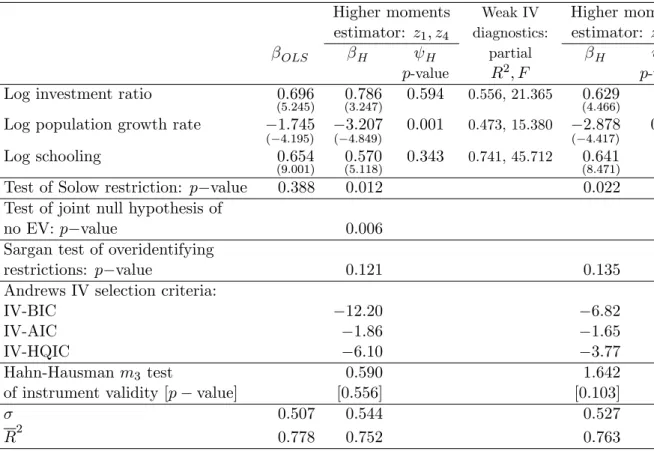
Tables 4 and 5 present our results for the MRW level regressions, while Tables 6 and 7 present our results for the growth regressions.15 Five aspects of the results presented in Table 4 are worth emphasizing. First, there is a strong indication of EV given the low p-value associated with the joint EV test, especially in light of the relatively low power of this test as revealed by our Montecarlo results. Second, it would appear that the coe¢ cient associated with the population growth plus technical change plus depreciation (n + g + ) variable is grossly underestimated (in absolute value) by OLS, and that this bias stems from EV on this variable. Third, our proposed instrument set appears to be reasonably orthogonal to the error term, as shown by the p-value associated with the Sargan test, and there is little indication of a weak instruments problem on the basis of the m3 test statistic. Fourth, the parameter restriction implied by the
human capital augmented Solow model is soundly rejected at the 1% level. Thus, although the
H estimate is in some sense less precise than the corresponding OLS estimate, the magnitude
of the EV in the MRW level equation is su¢ cient for us to be able to reject one of the key restrictions implied by the human capital augmented Solow model. This suggests, contrary to what is claimed by MRW, that the human capital augmented Solow model does not provide a good explanation for observed cross-country di¤erences in per capita GDP, once EV are taken into account.
Finally, the preceding results are con…rmed when we allow the log investment ratio and log schooling to act as their own instruments (RHS of the Table), as would seem reasonable on the basis of the individual t-tests for the presence of EV. The m3 test statistic rises slightly with
respect to the speci…cation in which all variables are allowed to be subject to EV, indicating that there may be a slight weak instruments problem in this speci…cation. On the other hand, all three Andrews IV selection criteria come down in favor of the speci…cation in which all variables are allowed to be subject to EV.
In Table 5, we impose the Solow restriction, despite its being rejected in Table 4. In this case, the joint EV test no longer rejects the null of the absence of EV. Note also that the
1 5
All data used in this paper are available publicly and the TSP code used in all computations is, of course, available upon request.
estimated standard errors using H are much larger, and that both the Sargan and the m3 test
statistics reject: this is a pattern that sometimes emerges when EV concerns are not present and one can rely on the OLS coe¢ cient estimates.16
3.1.2 Growth regressions
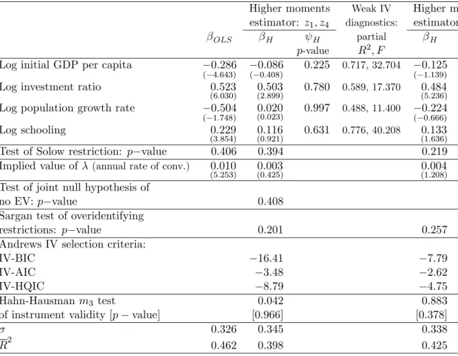
Table 6 presents the unrestricted growth regression results. When one allows all variables to be subject to EV, the joint EV test for the absence of EV does not reject. The standard errors of the H estimates are large when compared with their OLS counterparts and the point estimates of the coe¢ cients often fall substantially. However, both the Sargan and m3 test
statistics do not reject at the 10% level. In a second set of estimates, basing oneself on the individual t-tests for the presence of EV, all variables except the initial level of GDP per capita were allowed to act as their own instruments. In this case, the absence of EV on initial GDP per capita is strongly rejected (p-value = 0:029), while the Sargan and m3 test statistics
continue not to reject instrument validity. In comparison with the OLS results, these estimates based on the higher moments estimator yield a much lower annual rate of convergence, which is indistinguishable from zero at the usual levels of con…dence, as well as point estimates of the marginal impacts of the population growth rate and schooling that are 50% lower and also statistically indistinguishable from zero.
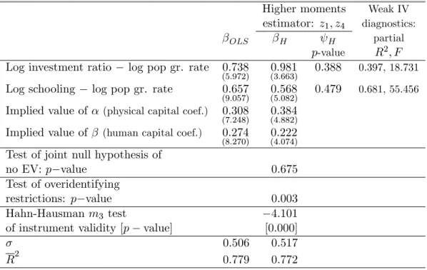
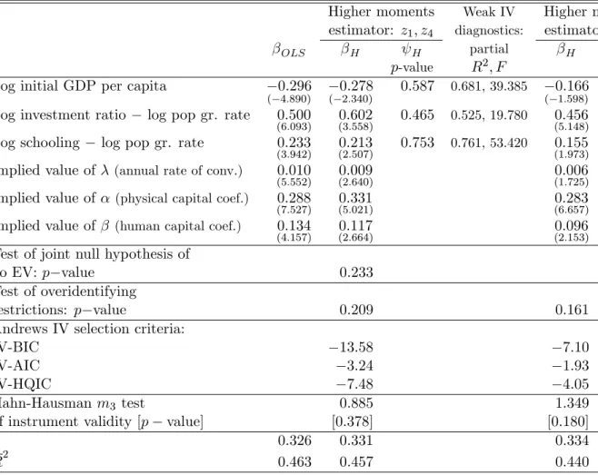
Given that the Solow restriction, in contrast to the level regressions, is not rejected in the results presented in Table 6, we present results for the restricted speci…cation in Table 7. As with the unrestricted speci…cation, it is only when initial GDP per capita is the only variable assumed to be a¤ected by EV that the EV test rejects. The gain in e¢ ciency furnished by the imposition of the Solow restriction allows one to obtain structural parameter estimates (of and ) that are measured relatively precisely and are of the same order of magnitude as those obtained using OLS. As with the unrestricted speci…cation, the main impact of EV is to bias the implied annual rate of convergence upward. Using OLS, one obtains OLS = 0:010
(t-statistic = 5:552) which is cut in half, to H = 0:006 (t-statistic = 1:725) once EV are controlled
for. Given our Montecarlo results concerning the relatively low levels of bias yielded by the higher moments estimator, we believe that the 0.006 …gure is likely to be closer to the actual annual rate of convergence than is the 0.010 …gure. Note also that our proposed instrument set is not rejected, either by the Sargan or the m3 test statistics.
1 6While these di¤erences between the results of our tests for the unrestricted versus the restricted regressions
may appear at …rst sight to be incoherent, they are readily explainable. Letye3 (here, the n + g + variable) be
measured with error: y3=ey3+ V, and suppose that the investment ratio variable, denoted by ey2, is measured
without signi…cant error (this is what is suggested by the corresponding p-values in Table 4). Assuming, for simplicity, that there is no correlation betweenye2 and y3 (the actual correlation is not zero, but it is very small)
the asymptotic bias of the OLS estimate of the coe¢ cient of y3would depend on the magnitude of 2V= 2y3whereas
the asymptotic bias of the coe¢ cient estimate in the restricted regression model — in this case the explanatory variable is (ey2 y3)— is given by 2V=( 2ey2+
2
y3):It follows, therefore, that
2 V=( 2ey2+ 2 y3) < 2 V= 2y3:Hence,
one would expect the OLS coe¢ cient on the restricted model to be less biased asymptotically. This explains our failure to reject the null hypothesis of no EV in the restricted regression, while our test detected EV in the unrestricted regressions.
3.2 Barro
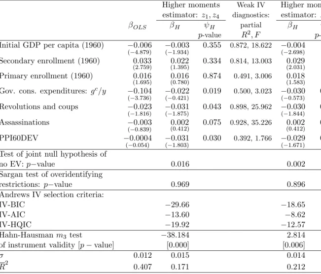
Tables 8 presents results for Barro, for the sample restricted to countries with initial GDP per capita (in 1960) greater than $1,000, which a priori should be less a¤ected by EV. The joint EV test rejects the null of the absence of EV, the Sargan test of the overidentifying restrictions does not reject, while the m3 test, taken in conjunction with the Sargan result, indicates that
our proposed instruments are weak.17 The H coe¢ cients associated with initial GDP per capita and government consumption expenditures fall substantially, in absolute value, with re-spect to the OLS results, with the t-statistic associated with gc=y going from t
OLS = 3:736 to
tH = 0:421.18 Barro’s explanation for the deleterious impact of government consumption
ex-penditures on economic growth was that “government consumption [as opposed to government investment] has no direct e¤ect on private productivity (or private property rights), but low-ered saving and growth through the distorting e¤ects from taxation or government-expenditure programs.” (p. 430) Our H results cast doubt on this …nding. Conversely, the absolute value of the coe¢ cient associated with PPI60DEV increases, as does the associated t-statistic.
In the RHS of the Table, initial GDP per capita and both enrollment rates are allowed to act as their own instruments, given the relatively high p-values on the associated individual tests for the absence of EV on these variables. The point estimates change very little, the coe¢ cient associated with government consumption expenditures continues to remain statisti-cally indistinguishable from zero, the Sargan test still does not reject, while the m3test statistic
falls substantially (though it remains statistically signi…cant at the usual levels of con…dence), indicating that a portion of the weak instruments problem has been eliminated, though there are still good reasons to continue implementing our IVs using the Fuller estimator.
3.3 Sachs and Warner
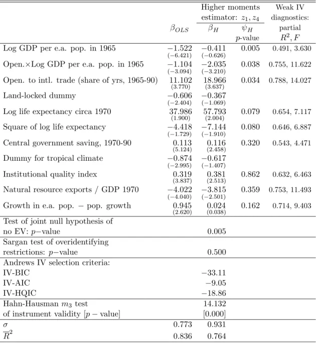
Results for SW are presented in Tables 9 and 10. In Table 9, the joint EV test rejects the absence of EV, the Sargan test does not reject our proposed instrument set, whereas the m3test
statistic indicates that our instruments are, however, weak. The H estimates of the coe¢ cients associated with initial GDP per economically active member of the population and the growth rate of the economically active population (minus the total growth rate of the population) fall substantially (in absolute value) and become statistically indistinguishable from zero. The H coe¢ cients associated with the landlocked and tropical climate dummies fall somewhat (both variables act as their own instruments) and are measured much less precisely than in the OLS case. All other coe¢ cients change relatively little and remain statistically signi…cant at the
1 7
Note also that the partial F -tests on the reduced forms for primary enrollment, government consumption expenditure, and PPI60DEV are all extremely low.
1 8
Note that we have found that correcting for EV using our higher moments estimator decreases the coe¢ cient on the initial level of GDP per capita, which would appear to contradict the received wisdom that EV biases coe¢ cients downwards. In reality, this nugget of received wisdom is, simply put, wrong. In a simple regression with a single explanatory variable, when there is measurement error on the said variable, the OLS estimator of the coe¢ cient associated with this variable is indeed asymptotically biased toward zero and this bias disappears when the true value of the coe¢ cient is zero. This is no longer the case, however, when there are several explanatory variables a¤ected by measurement errors, unless they are perfectly uncorrelated. The biases associated with errors of measurement can go in either direction for any given coe¢ cient, and this bias does not reduce to zero even if the true coe¢ cient is zero. See the illustration in Dagenais (1994), as well as the bias results from the Montecarlo experiments reported in Tables 2 and 3 of the present paper.
usual levels of con…dence.
In Table 10, we allow the institutional quality index and the growth rate of the economically active population to act as their own instruments, on the basis of the individual t-statistics for the presence of EV reported in the previous table. We continued to instrument central government saving and natural resource exports, despite the relatively high p-values of the individual test for EV associated with these variables presented in Table 10, because failure to do so resulted in a sound rejection of instrument validity by the Hahn-Hausman m3 test
statistic.
Two di¤erences with respect to the results presented in Table 9 are apparent. First, the dummy for a tropical climate returns (as in the OLS results) to being negative and statistically signi…cant. Second, and most importantly, instrument validity is not rejected by the m3
statistic.
The upshot is that, contrary to what is reported by SW, (i) there is no statistically signi…cant conditional convergence result, and (ii) being landlocked does not penalize countries in terms of their growth rate of GDP per capita, ceteris paribus. This last …nding casts doubt on one of the main empirical results advanced by proponents of the "geographical" (as opposed to "institutional") view of the determinants of economic growth.19
3.4 Easterly and Levine
Results for EL are presented in Tables 11 and 12. In Table 11 we present results in which only the decade and continent dummies are assumed to be measured without error. Point estimates change very little with respect to the OLS results, with the notable exception of the coe¢ cient associated with ethnolinguistic fragmentation, which becomes statistically insigni…cant. The joint test for the presence of EV, though it does not reject at the 10% level, suggests the presence of EV, especially when considered along with the individual t-tests for initial GDP per capita, the same variable squared, and ethnolinguistic fragmentation. On the other hand, the Sargan test rejects the validity of the overidentifying restrictions, whereas the m3 statistic suggests a
severe weak instruments problem.
In Table 12, we allow all variables, apart from initial GDP per capita and ethnolinguistic fragmentation, to act as their own instruments, on the basis of the individual t-tests for the presence of EV reported in Table 11. The di¤erences between the OLS and the H results, in terms both of the coe¢ cient estimates and the associated t-statistics, are extremely small, apart from ethnolinguistic fragmentation, for which the H coe¢ cient is half the value of its OLS counterpart and is statistically indistinguishable from zero. The joint EV test rejects the null of the absence of EV, the Sargan test does not reject (if one takes a 10% critical p-value) and, most importantly, the m3 test statistic does not reject. Our results based on the higher moments
estimator therefore suggest, contrary to the main argument given in EL, that ethnolinguistic fragmentation is not one of the main reasons behind the poor growth performance of sub-saharan Africa.
1 9Note that while all three Andrews IV selection criteria come down in favor of the estimates presented in
Table 9, the rejection of IV validity by the Hahn-Hausman test in Table 9 leads us to prefer the results presented in Table 10.
3.5 Levine and Zervos
Results for LZ are presented in Table 13. In the LHS of the table, we allow all variables to be a¤ected by EV. The point estimates change very little with respect to the OLS results, with the exception of government investment expenditures ("government", in the Table), which was statistically insigni…cant, at the usual levels of con…dence, in the OLS results, and becomes even less signi…cant once the H estimator is applied. The joint EV test does not reject, and the same is true of the test of the overidentifying restrictions and the Hahn-Hausman test.
On the basis of the individual t-tests for the presence of EV presented in the LHS of the Table, the RHS presents results in which only initial GDP per capita and government are allowed to be a¤ected by EV, with all other variables serving as their own instruments. Both the Sargan and the Hahn-Hausman tests fail to reject the null of instrument validity, while the p-value of the joint EV test falls substantially, with the individual test for EV on government becoming statistically signi…cant at the 10% level of con…dence. On the other hand, all other coe¢ cients are not signi…cantly di¤erent from their OLS counterparts, and it would therefore appear that the LZ results are not su¢ ciently a¤ected by an EV problem for it to be appropriate to prefer the H results to the original estimates based on OLS.
4
Concluding Remarks
In this paper we have subjected several well-known cross-sectional studies which propose a set of “stylized facts” regarding the determinants of the growth process to tests for the presence of EV in the explanatory variables. The implication of the results presented here is that EV can matter, and that several well-known "stylized facts" in the cross-sectional growth literature are not robust to controlling for EV. In particular, results such as the validity of the human capital-augmented Solow model (MRW), the deleterious impact of government consumption expenditures (Barro), the negative impact of being landlocked (SW), and the explanation for the low growth rate of sub-saharan Africa based on high levels of ethnolinguistic fragmentation (EL), are overturned once errors in variables are controlled for using our higher moments estimator.
While, as Robert Solow puts it, “few econometricians have ever been forced by the facts to abandon a …rmly held belief,” we believe that our paper indicates that further work on testing the robustness of results in the empirical growth literature using econometric methods which are robust to errors in variables is certainly warranted. This is particularly true in the context of panel data, since it is well-known that the usual covariance transformations, such as the "within" procedure or …rst-di¤erencing, often exacerbate problems of errors in variables, and that GMM procedures applied to …rst-di¤erenced data may not solve the problem when serial correlation is present.
References
Andrews, D. W. K. (1999): “Consistent Moment Selection Procedures for Generalized Method of Moments Estimation,” Econometrica, 67(3), 543–564.
Barro, R. J. (1991): “Economic Growth in a Cross Section of Countries,” Quarterly Journal of Economics, 106(2), 407–443.
Bound, J., D. A. Jaeger,andR. M. Baker (1995): “Problems with Instrumental Variables Estimation When the Correlation Between the Instruments and the Endogenous Explanatory Variable is Weak,” Journal of the American Statistical Association, 90(430), 443–450. Cruz, L. M., and M. J. Moreira (2005): “On the Validity of Econometric Techniques with
Weak Instruments. Inference on Returns to Education Using Compulsory School Attendance Laws,” The Journal of Human Resources, 40(2), 393–410.
Dagenais, M. G. (1994): “Parameter Estimation in Regression Models with Errors in the Variables and Autocorrelated Disturbances,” Journal of Econometrics, 64(1-2), 145–163. Dagenais, M. G., and D. L. Dagenais (1994): “GMM Estimators for Linear Regression
Models with Errors in Variables,” Cahier 9404, Département de sciences économiques, Uni-versité de Montréal.
(1997): “Higher Moment Estimators for Linear Regression Models with Errors in the Variables,” Journal of Econometrics, 76(1-2), 193–221.
Donald, S. A., and W. K. Newey (2001): “Choosing the Number of Instruments,” Econo-metrica, 69(5), 1161–1191.
Drion, E. F. (1951): “Estimation of the Parameters of a Straight Line and of the Variance of the Variables, If They Are Both Subject to Error,”Indagationes Mathematicae, 13, 256–260. Easterly, W. R., and R. Levine (1997): “Africa’s Growth Tragedy: Policies and Ethnic
Divisions,” Quarterly Journal of Economics, 112(4), 1203–1250.
Edwards, S. (1993): “Openness, Trade Liberalization, and Growth in Developing Countries,” Journal of Economic Literature, 31(3), 1358–1393.
Fuller, W. A. (1977): “Some Properties of a Modi…cation of the Limited Information Esti-mator,” Econometrica, 45(4), 939–954.
Geary, R. C. (1942): “Inherent Relations Between Random Variables,” Proceedings of the Royal Irish Academy, 47, 63–76.
Hahn, J., and J. A. Hausman (2002a): “A New Speci…cation Test for the Validity of Instru-mental Variables,” Econometrica, 70(1), 163–189.
(2002b): “Notes on Bias in Estimators for Simultaneous Equation Models,”Economics Letters, 75(2), 237–241.
(2003): “Weak Instruments: Diagnosis and Cures in Empirical Econometrics,” Amer-ican Economic Review, 93(2), 118–125.
Hahn, J., J. A. Hausman, and G. Kuersteiner (2004): “Estimation with Weak Instru-ments: Accuracy of Higher Order Bias and MSE Approximations,” Econometrics Journal, 7(1), 272–306.
Hausman, J. A. (1978): “Speci…cation Tests in Econometrics,” Econometrica, 46(6), 1251– 1272.
Hausman, J. A., J. H. Stock, and M. Yogo (2004): “Asymptotic Properties of the Hahn-Hausman Test for Weak Instruments,” processed, Department of Economics, MIT and Har-vard.
Kendall, M. G., and A. Stuart (1963): The Advanced Theory of Statistics, vol. 1. Charles Gri¢ n and Company, London, UK, second edn.
Klepper, S., and E. Leamer (1984): “Consistent Sets of Estimates for Regressions with Errors in All Variables,” Econometrica, 52(1), 163–183.
Langaskens, Y.,andM. Van Rickeghem (1974): “A New Method to Estimate Measurement Errors in National Income Account Statistics: The Belgian Case,” International Statistical Review, 42(3), 283–290.
Levine, D., and D. Renelt (1992): “A Sensitivity Analysis of Cross Country Growth Re-gressions,” American Economic Review, 82(4), 942–963.
Levine, R.,andS. Zervos (1998): “Stock Markets, Banks, and Economic Growth,”American Economic Review, 88(3), 537–558.
Lipsey, R. E., and H. S. Tice (eds.) (1989): The Measurement of Saving, Investment, and Wealth, National Bureau of Economic Research Studies in Income and Wealth. University of Chicago Press, Chicago, IL.
Malinvaud, E. (1978): Méthodes Statistiques de l’Econométrie. Dunod, Paris, France, third edn.
Mankiw, N. G., D. Romer, and D. Weil (1992): “A Contribution to the Empirics of Economic Growth,” Quarterly Journal of Economics, 107(2), 407–437.
Morgenstern, O. (1963): On the Accuracy of Economic Observations. Princeton University Press, Princeton, NJ, second edn.
Nelson, D. (1995): “Vector Attenuation Bias in the Classical Errors-in-Variables Model,” Economics Letters, 49(4), 345–349.
Pal, M. (1980): “Consistent Moment Estimators of Regression Coe¢ cients in the Presence of Errors in Variables,” Journal of Econometrics, 14(3), 349–364.
Sachs, J. D., and A. M. Warner (1997a): “Fundamental Sources of Long-Run Growth,” American Economic Review, 87(2), 184–188.
(1997b): “Sources of Slow Growth in African Economies,” Journal of African Economies, 6(3), 335–376.
Shea, J. (1997): “Instrument Relevance in Multivariate Linear Models: A Simple Measure,” Review of Economics and Statistics, 79(2), 348–352.
Srinivasan, T. N. (1994): “Data Base for Development Analysis: An Overview,” Journal of Development Economics, 44(1), 3–27.
Stock, J. H., J. T. Wright, and M. Yogo (2002): “A Survey of Weak Instruments and Weak Identi…cation in Generalized Methods of Moments,”Journal of Business and Economic Statistics, 20(4), 518–529.
Temple, J. (1998): “Robustness Tests of the Augmented Solow Model,” Journal of Applied Econometrics, 13(4), 361–375.
White, H. (1980): “A Heteroskedasticity-Consistent Covariance Matrix Estimator and a Direct Test for Heteroskedasticity,” Econometrica, 48(4), 817–838.
Paper Joint null of Some point Basic result the absence of estimates of paper measurement signi…cantly that is
error changed overturned
Barro rejected yes government
1991 consumption
expenditures no longer signi…cant
MRW (levels) rejected yes human capital
1992 augmented Solow
model rejected
MRW (growth) not rejected yes annual rate of
1992 convergence
halved
Sachs-Warner rejected yes landlocked dummy
1997 and initial GDP
per capita no longer signi…cant
Easterly-Levine rejected yes ethnolinguitic
1997 diversity no
longer signi…cant
Levine-Zervos not rejected no none
1998
Table 1: A summary of our results concerning measurement error in cross-sectional growth regressions
Coe¢ cient OLS H
z1 and z4 z1 through z7
all vars. onlyy3 all vars. onlyy3
instru- instru- instru-
instru--mented -mented -mented -mented
Biases
0 0:230 0:047 0:066 0:077 0:242
2 0:073 0:010 0:020 0:025 0:079
3 0:334 0:080 0:098 0:119 0:347
4 0:122 0:030 0:038 0:031 0:128
Average of absolute values 0:190 0:042 0:056 0:063 0:199
Root mean-squared errors
0 0:397 0:691 0:519 1:381 0:782
2 0:268 0:439 0:297 0:740 0:358
3 0:376 0:653 0:600 1:553 1:020
4 0:168 0:252 0:238 0:568 0:377
Average RMSEs 0:302 0:509 0:414 1:061 0:634
Size of type I errors, %
0 0:105 0:036 0:038 0:126 0:112
2 0:056 0:035 0:038 0:087 0:047
3 0:491 0:047 0:045 0:227 0:219
4 0:191 0:043 0:045 0:152 0:165
Average size of type I errors 0:211 0:040 0:041 0:148 0:136
Power of EV test 0:164 0:138 0:164 0:138
"True" relationship: y1 = 1 +ye2+ey3+ye4+ u;
variable a¤ected by EV: y3=ye3+ V;
experiment carried out with 98 observations, R2 = 0:778; ratio of variance of V to variance of ye3 equal to 0:3,
"true" size of type I errors equal to 0:05, and 5000 replications.
Coe¢ cient OLS H z1 and z4 z1 through z7 Biases 0 0:390 0:152 0:116 2 0:158 0:064 0:026 3 0:391 0:148 0:151 4 0:204 0:073 0:074
Average of absolute values 0:286 0:110 0:091
Root mean-squared errors
0 0:513 0:776 1:590
2 0:366 0:598 1:076
3 0:408 0:523 1:262
4 0:235 0:286 0:674
Average RMSEs 0:381 0:546 1:151
Size of type I errors, %
0 0:199 0:049 0:125
2 0:066 0:039 0:086
3 0:893 0:092 0:208
4 0:398 0:068 0:143
Average size of type I errors 0:389 0:062 0:141
Power of EV test 0:227 0:227
"True" relationship: y1 = 1 +ye2+ey3+ (0 ey4) + u;
variable a¤ected by EV: y3=ye3+ V;
experiment carried out with 98 observations, R2 = 0:592; ratio of variance of V to variance of ye3 equal to 0:8,
"true" size of type I errors equal to 0:05, and 5000 replications.
Higher moments Weak IV Higher moments Weak IV
estimator: z1; z4 diagnostics: estimator: z1; z4 diagnostics: OLS H H partial H H partial
p-value R2; F p-value R2; F
Log investment ratio 0:696
(5:245) 0:786(3:247) 0.594 0.556, 21.365 (4:466)0:629
Log population growth rate 1:745
( 4:195) 3:207 ( 4:849) 0.001 0.473, 15.380 2:878 ( 4:417) 0.014 0.397, 57.483 Log schooling 0:654 (9:001) 0:570(5:118) 0.343 0.741, 45.712 (8:471)0:641
Test of Solow restriction: p value 0:388 0:012 0:022
Test of joint null hypothesis of
no EV: p value 0:006
Sargan test of overidentifying
restrictions: p value 0:121 0:135
Andrews IV selection criteria:
IV-BIC 12:20 6:82
IV-AIC 1:86 1:65
IV-HQIC 6:10 3:77
Hahn-Hausman m3 test 0:590 1:642
of instrument validity [p value] [0:556] [0:103]
0:507 0:544 0:527
R2 0:778 0:752 0:763
Table 4: MRW 1992. Dependent variable: GDP per capita in 1985, unrestricted speci…cation, 98 observations (t-statistics in parentheses unless otherwise noted)
Higher moments Weak IV
estimator: z1; z4 diagnostics: OLS H H partial
p-value R2; F Log investment ratio log pop gr. rate 0:738
(5:972) 0:981(3:663) 0.388 0.397, 18.731
Log schooling log pop gr. rate 0:657
(9:057) 0:568(5:082) 0.479 0.681, 55.456
Implied value of (physical capital coef.) 0:308
(7:248) 0:384(4:882)
Implied value of (human capital coef.) 0:274
(8:270) 0:222(4:074)
Test of joint null hypothesis of
no EV: p value 0:675
Test of overidentifying
restrictions: p value 0:003
Hahn-Hausman m3 test 4:101
of instrument validity [p value] [0:000]
0:506 0:517
R2 0:779 0:772
Table 5: MRW 1992. Dependent variable: GDP per capita in 1985, restricted speci…cation, 98 observations (t-statistics in parentheses unless otherwise noted)
Higher moments Weak IV Higher moments Weak IV
estimator: z1; z4 diagnostics: estimator: z1; z4 diagnostics: OLS H H partial H H partial
p-value R2; F p-value R2; F
Log initial GDP per capita 0:286
( 4:643) 0:086 ( 0:408) 0.225 0.717, 32.704 0:125 ( 1:139) 0.029 0.200, 21.453
Log investment ratio 0:523
(6:030) (2:899)0:503 0.780 0.589, 17.370 (5:236)0:484
Log population growth rate 0:504
( 1:748)
0:020
(0:023) 0.997 0.488, 11.400 ( 0:666)0:224
Log schooling 0:229
(3:854) (0:921)0:116 0.631 0.776, 40.208 (1:636)0:133
Test of Solow restriction: p value 0:406 0:394 0:219
Implied value of (annual rate of conv.) 0:010
(5:253) (0:425)0:003 (1:208)0:004
Test of joint null hypothesis of
no EV: p value 0:408
Sargan test of overidentifying
restrictions: p value 0:201 0:257
Andrews IV selection criteria:
IV-BIC 16:41 7:79
IV-AIC 3:48 2:62
IV-HQIC 8:79 4:75
Hahn-Hausman m3 test 0:042 0:883
of instrument validity [p value] [0:966] [0:378]
0:326 0:345 0:338
R2 0:462 0:398 0:425
Table 6: MRW 1992. Dependent variable: Growth rate of GDP per capita, 1960-1985, unrestricted speci…cation, 98 observations (t-statistics in parentheses unless otherwise noted)
Higher moments Weak IV Higher moments Weak IV
estimator: z1; z4 diagnostics: estimator: z1; z4 diagnostics: OLS H H partial H H partial
p-value R2; F p-value R2; F
Log initial GDP per capita 0:296
( 4:890) 0:278 ( 2:340) 0.587 0.681, 39.385 0:166 ( 1:598) 0.044 0.242, 26.141
Log investment ratio log pop gr. rate 0:500
(6:093) (3:558)0:602 0.465 0.525, 19.780 (5:148)0:456
Log schooling log pop gr. rate 0:233
(3:942) (2:507)0:213 0.753 0.761, 53.420 (1:973)0:155
Implied value of (annual rate of conv.) 0:010
(5:552) (2:640)0:009 (1:725)0:006
Implied value of (physical capital coef.) 0:288
(7:527) (5:021)0:331 (6:657)0:283
Implied value of (human capital coef.) 0:134
(4:157) (2:664)0:117 (2:153)0:096
Test of joint null hypothesis of
no EV: p value 0:233
Test of overidentifying
restrictions: p value 0:209 0:161
Andrews IV selection criteria:
IV-BIC 13:58 7:10
IV-AIC 3:24 1:93
IV-HQIC 7:48 4:05
Hahn-Hausman m3 test 0:885 1:349
of instrument validity [p value] [0:378] [0:180]
0:326 0:331 0:334
R2 0:463 0:457 0:440
Table 7: MRW 1992. Dependent variable: Growth rate of GDP per capita, restricted speci…cation, 1960-1985, 98 observations (t-statistics in parentheses unless otherwise noted)
Higher moments Weak IV Higher moments Weak IV
estimator: z1; z4 diagnostics: estimator: z1; z4 diagnostics: OLS H H partial H H partial
p-value R2; F p-value R2; F Initial GDP per capita (1960) 0:006
( 4:879) 0:003 ( 1:934) 0.355 0.872, 18.622 0:004 ( 2:698) Secondary enrollment (1960) 0:033 (2:759) (1:395)0:022 0.334 0.814, 13.003 0:029(2:031) Primary enrollment (1960) 0:016 (1:695) (0:780)0:016 0.874 0.491, 3.006 0:018(1:583)
Gov. cons. expenditures: gc=y 0:104
( 3:736) 0:022 ( 0:421) 0.019 0.500, 3.023 0:030 ( 0:573) 0.035 0.402, 3.711
Revolutions and coups 0:023
( 1:816) 0:031 ( 1:875) 0.043 0.898, 25.962 0:030 ( 1:844) 0.039 0.803, 23.380 Assassinations 0:003 ( 0:839) 0:002 (0:412) 0.075 0.928, 35.226 0:002(0:412) 0.023 0.867, 37.649 PPI60DEV 0:0004 ( 0:054) 0:031 ( 1:803) 0.030 0.392, 1.766 0:029 ( 1:671) 0.023 0.310, 2.609
Test of joint null hypothesis of
no EV: p value 0:016 0:002
Sargan test of overidentifying
restrictions: p value 0:969 0:896
Andrews IV selection criteria:
IV-BIC 29:66 18:65
IV-AIC 13:60 8:62
IV-HQIC 19:92 12:57
Hahn-Hausman m3 test 38:184 2:814
of instrument validity [p value] [0:000] [0:006]
0:012 0:015 0:014
R2 0:407 0:171 0:212
Table 8: Barro (1991). Dependent variable: growth rate of GDP per capita, 1960-85, GDP per capita in 1960 > 1,000 dollars, 55 observations (t-statistics in parentheses unless otherwise noted)
Higher moments Weak IV
estimator: z1; z4 diagnostics: OLS H H partial
p-value R2; F
Log GDP per e.a. pop. in 1965 1:522
( 6:421)
0:411
( 0:626)
0.005 0.491, 3.630
Open. Log GDP per e.a. pop. in 1965 1:104
( 3:094)
2:035
( 3:210)
0.038 0.755, 11.622
Open. to intl. trade (share of yrs, 1965-90) 11:102
(3:770) 18:966(3:637) 0.034 0.788, 14.027
Land-locked dummy 0:606
( 2:404)
0:367
( 1:069)
Log life expectancy circa 1970 37:986
(1:900) 57:793(2:004) 0.079 0.654, 7.117
Square of log life expectancy 4:418
( 1:729)
7:144
( 1:910)
0.080 0.646, 6.887
Central government saving, 1970-90 0:113
(5:124) (2:458)0:116 0.320 0.543, 4.471
Dummy for tropical climate 0:874
( 2:995)
0:617
( 1:407)
Institutional quality index 0:319
(3:837) (2:513)0:381 0.862 0.632, 6.463
Natural resource exports / GDP 1970 4:022
( 4:040)
3:815
( 2:501)
0.359 0.753, 11.493
Growth in e.a. pop. pop. growth 0:945
(2:620) (0:038)0:024 0.162 0.714, 9.403
Test of joint null hypothesis of
no EV: p value 0:005
Sargan test of overidentifying
restrictions: p value 0:500
Andrews IV selection criteria:
IV-BIC 33:11
IV-AIC 9:05
IV-HQIC 18:86
Hahn-Hausman m3 test 14:132
of instrument validity [p value] [0:000]
0:773 0:931
R2 0:836 0:764
Table 9: Sachs-Warner 1997. Dependent variable: growth rate of per capita PPP-adjusted GDP, 1965-1990, 82 observations (t-statistics in parentheses unless otherwise noted)
Higher moments Weak IV
estimator: z1; z4 diagnostics: OLS H H partial
p-value R2; F
Log GDP per e.a. pop. in 1965 1:522
( 6:421)
0:344
( 0:440)
0.002 0.413, 3.693
Open. Log GDP per e.a. pop. in 1965 1:104
( 3:094)
1:624
( 2:992)
0.006 0.620, 8.522
Open. to intl. trade (share of yrs, 1965-90) 11:102
(3:770) 15:666(3:447) 0.007 0.680, 11.124
Land-locked dummy 0:606
( 2:404)
0:313
( 0:894)
Log life expectancy circa 1970 37:986
(1:900) 34:981(1:440) 0.125 0.529, 5.883
Square of log life expectancy 4:418
( 1:729)
4:381
( 1:387)
0.126 0.525, 5.795
Central government saving, 1970-90 0:113
(5:124) (2:417)0:124 0.634 0.483, 4.894
Dummy for tropical climate 0:874
( 2:995)
0:849
( 2:101)
Institutional quality index 0:319
(3:837) (2:370)0:250
Natural resource exports / GDP 1970 4:022
( 4:040)
3:550
( 2:277)
0.479 0.735, 14.538
Growth in e.a. pop. pop. growth 0:945
(2:620) (2:386)1:051
Test of joint null hypothesis of
no EV: p value 0:003
Sargan test of overidentifying
restrictions: p value 0:112
Andrews IV selection criteria:
IV-BIC 20:60
IV-AIC 1:35
IV-HQIC 9:20
Hahn-Hausman m3 test 0:849
of instrument validity [p value] [0:398]
0:773 0:913
R2 0:836 0:773
Table 10: Sachs-Warner 1997. Dependent variable: growth rate of per capita PPP-adjusted GDP, 1965-1990, 82 observations (t-statistics in parentheses unless otherwise noted)
Higher moments Weak IV estimator: z1; z4 diagnostics: OLS H H partial p-value R2; F 1960s 0:320 ( 3:119) 0:335 ( 3:045) 1970s 0:313 ( 3:054) 0:329 ( 3:000) 1980s 0:328 ( 3:196) 0:344 ( 3:137) Sub-saharan Africa 0:012 ( 2:391) 0:015 ( 2:170) Latin America 0:019 ( 5:421) 0:018 ( 5:069)
Log initial GDP per capita 0:104
(4:044) (3:886)0:108 0.023 0.756, 28.570
Log initial GDP per capita, squared 0:007
( 4:732) 0:008 ( 4:204) 0.023 0.755, 28.290 Log schooling 0:010 (2:223) (1:391)0:010 0.862 0.585, 13.053 Assassinations 18:519 ( 2:037) 16:666 ( 1:760) 0.344 0.893, 72.791 Financial depth 0:012 (2:121) (1:387)0:011 0.694 0.733, 24.919
Black market premium 0:018
( 4:087) 0:017 ( 3:429) 0.146 0.837, 46.825 Fiscal surplus 0:194 (5:243) (2:553)0:165 0.793 0.366, 5.305 Ethnolinguistic fragmentation 0:012 ( 1:849) 0:004 ( 0:481) 0.069 0.670, 18.824
Log telephones per worker 0:005
(1:827) (1:079)0:007 0.551 0.694, 20.901
Test of joint null hypothesis of
no EV: p value 0.124
Sargan test of overidentifying
restrictions: p value 0.026
Andrews IV selection criteria:
IV-BIC 31:17
IV-AIC 0:46
IV-HQIC 12:53
Hahn-Hausman m3 test 436:837
of instrument validity [p value] [0:000]
0.016 0.016
R2 0.581 0.574
Table 11: Easterly-Levine 1997. Dependent variable: growth rate of GDP per capita, 1960-90, 175 observations (t-statistics in parentheses unless otherwise noted)
Higher moments Weak IV estimator: z1; z4 diagnostics: OLS H H partial p-value R2; F 1960s 0:320 ( 3:119) 0:342 ( 3:293) 1970s 0:313 ( 3:054) 0:335 ( 3:229) 1980s 0:328 ( 3:196) 0:350 ( 3:370) Sub-saharan Africa 0:012 ( 2:391) 0:014 ( 2:650) Latin America 0:019 ( 5:421) 0:018 ( 5:255)
Log initial GDP per capita 0:104
(4:044) (4:203)0:110 0.033 0.318, 15.711
Log initial GDP per capita, squared 0:007
( 4:732) 0:008 ( 4:902) 0.033 0.307, 14.983 Log schooling 0:010 (2:223) (2:092)0:009 Assassinations 18:519 ( 2:037) 19:416 ( 2:127) Financial depth 0:012 (2:121) (2:153)0:012
Black market premium 0:018
( 4:087) 0:018 ( 3:957) Fiscal surplus 0:194 (5:243) (5:349)0:199 Ethnolinguistic fragmentation 0:012 ( 1:849) 0:006 ( 0:868) 0.090 0.602, 50.845
Log telephones per worker 0:005
(1:827) (2:131)0:006
Test of joint null hypothesis of
no EV: p value 0.058
Sargan test of overidentifying
restrictions: p value 0.132
Andrews IV selection criteria:
IV-BIC 14:57
IV-AIC 1:91
IV-HQIC 7:11
Hahn-Hausman m3 test 0:223
of instrument validity [p value] [0:823]
0.016 0.016
R2 0.581 0.579
Table 12: Easterly-Levine 1997. Dependent variable: growth rate of GDP per capita, 1960-90, 175 observations (t-statistics in parentheses unless otherwise noted)
Higher moments Weak IV Higher moments Weak IV
estimator: z1; z4 diagnostics: estimator: z1; z4 diagnostics: OLS H H partial H H partial
p-value R2; F p-value R2; F
Log initial GDP per capita 0:013
( 3:287) 0:018 ( 3:486) 0.276 0.883, 12.137 0:016 ( 3:027) 0.209 0.200, 3.142
Log secondary enrollment 0:023
(2:599) 0:031(2:900) 0.353 0.916, 16.847 0:024(2:267)
Revolutions and coups 0:034
( 2:872) 0:034 ( 2:605) 0.952 0.953, 30.251 0:034 ( 2:754) Government 0:061 ( 1:319) 0:009 ( 0:142) 0.252 0.764, 5.542 0:013 ( 0:220) 0.086 0.538, 12.674 In‡ation 0:007 ( 0:525) 0:0008 ( 0:058) 0.545 0.956, 36.714 0:004 ( 0:289)
Black market premium 2 10 5
( 0:322) 3 10 6 (0:044) 0.841 0.991, 162.716 2 10 5 ( 0:348) Bank credit 0:013 (1:492) 0:016(1:502) 0.939 0.883, 12.852 0:016(1:799) Turnover 0:026 (2:466) 0:020(1:698) 0.992 0.928, 20.850 0:026(2:333)
Test of joint null hypothesis of
no EV: p value 0.807 0.158
Sargan test of overidentifying
restrictions: p value 0.330 0.991
Andrews IV selection criteria:
IV-BIC 21:63 11:18
IV-AIC 5:99 5:97
IV-HQIC 11:84 7:92
Hahn-Hausman m3 test 1:052 0:787
of instrument validity [p value] [0:298] [0:436]
0.017 0.018 0.018
R2 0.383 0.335 0.361
Table 13: Levine-Zervos (1998). Dependent variable: growth rate of GDP per capita, 1976-1993, 42 observations (t-statistics in parentheses unless otherwise noted)