HAL Id: hal-03022995
https://hal.archives-ouvertes.fr/hal-03022995
Preprint submitted on 25 Nov 2020
HAL is a multi-disciplinary open access
archive for the deposit and dissemination of
sci-entific research documents, whether they are
pub-lished or not. The documents may come from
teaching and research institutions in France or
abroad, or from public or private research centers.
L’archive ouverte pluridisciplinaire HAL, est
destinée au dépôt et à la diffusion de documents
scientifiques de niveau recherche, publiés ou non,
émanant des établissements d’enseignement et de
recherche français ou étrangers, des laboratoires
publics ou privés.
To cite this version:
Francesco Cairo, Mauro de Muro, Marcel Snels, Luca Liberto, Silvia Bucci, et al.. Lidar observations
of Cirrus clouds at Palau island (7
• 33 N, 134 • 48 E). 2020. �hal-03022995�
Lidar observations of Cirrus clouds at Palau island (7
◦
33
0
N,
134
◦
48
0
E)
Francesco Cairo
1, Mauro De Muro
1,2, Marcel Snels
1, Luca Di Liberto
1, Silvia Bucci
3, Bernard Legras
3,
Ajil Kottayil
4, Andrea Scoccione
1,5, and Stefano Ghisu
61Institute of Atmospheric and Climate Sciences, National Research Council of Italy (CNR), I-00133, Roma, Italy 2Now at: : AIT Thales Alenia Space, Roma, Italy
3Laboratoire de Météorologie Dynamique (LMD), UMR CNRS 8539, CNRS, IPSL, ENS-PSL, École Polytechnique, Sorbonne Université, Paris, France
4Advanced Centre for Atmospheric Radar Research, Cochin University of Science and Technology, Cochin, India 5Now at: Centro Operativo per la Meteorologia, Aeronautica Militare, Pomezia, Italy
6Università degli Studi di Roma "Tor Vergata", Dipartimento di Fisica, Roma, Italy Correspondence: Francesco Cairo (f.cairo@isac.cnr.it)
Abstract. A polarization diversity elastic backscatter lidar has been deployed in the equatorial island of Palau in February and March 2016, in the framework of the EU Stratoclim project. The system operated unattended in the Atmospheric Observatory of Palau Island from 15 February to 25 March 2016, during nighttime. Each lidar profile extends from the ground to 30 km height. Here the dataset is presented and discussed in terms of the temperature structure of the UTLS, obtained from co-located radiosondings. During the campaign, several high altitude clouds were observed, peaking approximately 3 km below the Cold
5
Point Tropopause (CPT) located above 17 km. Their occurrence was associated with cold anomalies in the Upper Troposphere (UT). Conversely, when warm UT anomalies occurred, the presence of cirrus was restricted to a 5 km thick layer centered 5 km below the CPT. Thin and subvisible cirrus were frequently detected close to the CPT. The particle depolarization ratios of these cirrus was generally lower than the values detected in the UT clouds. CPT cirrus occurrence showed a correlation with cold anomalies likely triggered by stratospheric wave activity penetrating the UT. The back trajectories study revealed a thermal and
10
convective history compatible with the convective outflow formation for most of the cirrus clouds, suggesting that the majority of air masses related to the clouds had encountered convection in the past and had reached the minimum temperature during its transport in less than 48 hours before the observation. A subset of SVC, with low depolarization and high lidar ratio and with no sign of significative recent uplifting, may be originated in situ.
1 Introduction
Cirrus are clouds composed of ice particles which form in the upper troposphere, covering about 20–25 % of the Earth (Rossow and Schiffer, 1999). They play an important role in climate: cirrus control the amount of solar radiative energy reaching the
ground, reflecting a fraction of the incident sunlight back to space; they also absorb infrared radiation, thus modulating the loss to space of the energy emitted from the surface and lower atmosphere. For their relevant role and feedbacks on climate, cirrus
20
have raised attention since long (Ramanathan and Collins, 1991). Moreover, cirrus are an essential modulator of the water budget in the upper troposphere and in the stratosphere: by condensing water vapour and removing it by particle gravitational settling, these clouds can dehydrate the upper layers of the troposphere and influence the amount of water vapor reaching the stratosphere, a most important role especially in the Tropics where the penetration of tropospheric air into the Stratosphere finds itself in the ascending branch of the Brewer-Dobson circulation, therefore impacting the Stratosphere as a whole. Their
25
radiative properties and dehydration potential depend critically on their microphysical properties, i.e. ice particles size, shape and number density, which are determined by environmental conditions (water vapor abundance, temperature and dynamics of the airmass where they reside) and formation mechanisms. Sassen and Cho (1992) suggest subdividing cirrus according to their optical thickness τ into subvisible (SVC), thin and opaque (τ < 0.03, 0.03 < τ < 0.3 and τ > 0.3, respectively). Most of the thin and SVC cirrus clouds occur in the Tropics and are more frequent at night and over the ocean. In the Tropics, cirrus often appear
30
to be associated with convective activity, with the likely exception of some of the highest ones in the Tropical Tropopause Layer (TTL). The TTL is a transition region a few kilometers thick that separates the Troposphere and the Stratosphere and is characterized by a radiatively driven slow ascent, and thus considered to be a processing region for tropospheric air to enter the stratosphere (Fueglistaler et al., 2009). There, the presence of cirrus clouds is of particular interest as they both modify the energy budget of the region through their radiative properties (Fu et al., 2018) and the release or uptake of latent heat upon their
35
formation or dissipation (Spichtinger, 2014). Moreover they can process tropospheric air both chemically and microphysically, altering the water vapour budget of the layer (Flury et al., 2011) and eventually of the stratosphere as a whole.
There are basically two kind of processes responsible for the formation of cirrus, namely in situ and convective formation. The first process is triggered by cooling from both large-scale vertical uplifting (Jensen et al., 1996; Pfister et al., 2001) and atmospheric Kelvin or gravity wave activity (Immler et al., 2008; Fujiwara et al., 2009). Upon cooling, ice particles
40
may directly form by either homogeneous and/or heterogeneous nucleation. Krämer et al. (2015) suggests considering two subclasses depending on the strength of the updraft and hence the rapidity of the cooling; slow updrafts tend to produce thinner cirrus with lower Ice Water Content (IWC), while faster updrafts form thicker cirrus with higher IWCs. In the second process cirrus are formed when deep convective mixed phase clouds deliver particles directly into the upper troposphere (Pfister et al., 2001; Comstock and Jakob, 2004) where the temperature is low enough (< 235 K) to allow for the full freezing of the liquid
45
droplets. These convectively generated cirrus are generally thicker than those formed by in situ mechanisms.
Lidar techniques can detect thin and SVC cirrus with high spatial and temporal resolution, providing accurate information on their geometrical and optical properties. Lidar backscattering ratio can be associated with cirrus microphysical bulk properties (Cairo et al., 2011) and lidar depolarization and extinction-to-backscatter ratio (a.k.a. lidar ratio, LR), with the average particle shape and phase, albeit with some caveats (Chen et al., 2002; Del Guasta, 2001; Reichardt et al., 2002).
50
The first report of lidar measurements of high tropical cirrus clouds, extending from 12 to 18 km with geometrical thickness less than 1 km, are by Uthe et al. (1977) from Kwajalein island (8◦70 N, 116◦70 E). Platt et al. (1987) compared tropical (Darwin 12◦80 S, 130◦70E) and midlatitude (Aspendale 38◦00 S, 144◦00) cirrus using the LIRAD method and finding less
variability in depolarization and greater optical thickness at lower temperatures in tropical cirrus clouds; in later measurements from Kavieng (2◦500S, 152◦70E) Platt et al. (1998) reported a decrease of the lidar integrated attenuated depolarization ratio
55
with temperature, from 0.42 at -70◦C to 0.18 at -10◦C, which actually contradicts some later findings. For instance, Sassen and Benson (2001) show for midlatitude cirrus a quite regular increase for decreasing temperatures, from values around 0.3 at 240 K to 0.45 at 195 K; depolarization measurements from Mahe (4.4◦S, 55.3◦E) from Pace et al. (2003) do not show a regular behavior in temperature, while in observations from Gadanki (13.5◦N, 79.2◦E) Sunilkumar and Parameswaran (2005) observed an increase with decreasing temperature, albeit in both cases the depolarization dropped to its lowest values at the
60
lowest temperatures (i.e. highest altitudes) observed. These apparently contradictory findings suggest that there may not be an univocal relationship between temperature and depolarization, as the latter may be influenced by the history rather than the instantaneous value of the air mass temperature, with high depolarization produced by fresh particles in cirrus clouds originating from the outflow of convective cells and intermediate to low depolarization associated with aged outflows and in situ formed cirrus, the latter often in the form of SVC, dwelling at or slightly below the Tropopause, as suggested by Pace et al.
65
(2003). Cirrus at the tropical tropopause are of particular interest as they represent the last thermodynamic process of water vapor before it enters the Stratosphere. Nee et al. (1998) recorded the presence of high tropospheric SVC, often showing an optical thickness of less than 0.01, at Chung-Li (25◦N, 121◦E), for almost 50% of the observational period between May and September 1993–95. Boehm and Verlinde (2000) related the occurrences of high and persistent cirrus clouds in Nauru (0.5◦S, 170◦E) to the temperature perturbation induced by equatorial Kelvin waves. The role of Kelvin as well as gravity- and Rossby
70
waves and their link to extensive, persistent laminar cirrus has then been addressed extensively (Pfister et al., 2001; Garrett et al., 2004). Wang et al. (2019) shows from 10 years of lidar satellite observations that these optically thin laminar cirrus occurs frequently in the west/central tropical Pacific, equatorial western Africa, and northern South America, thus preferably in the tropical large-scale ascending zones. Similarly, Wang and Dessler (2012) have shown with satellite observations that the convective fractions of cirrus increase with height until the cold point tropopause is reached, peaking in their geographical
75
occurrence over equatorial Africa, the tropical western Pacific, and South America. They have reported at least ∼30 % of cirrus in the TTL are of convective origin. Some studies have focused on the western Pacific tropical warm pool (TWP) (Platt et al., 2002; Heymsfield et al., 1998; Sassen et al., 2000; Comstock et al., 2002). They have reported that there thin cirrus are particularly frequent and can cover more than 50 % of the area (Prabhakara et al., 1993; Dessler and Yang, 2003).
This area, which spans the western waters of the equatorial Pacific, is characterised by a mean sea surface temperature (SST)
80
exceeding 28◦C, weak trade winds, deep convection extending above 15 km, and holds the warmest seawaters in the world. It has a large effect on surrounding monsoon regions and on climate so as to be called the “heat engine of the world” influencing remote regions and large scale weather variability (De Deckker, 2016). It is also a region of primary importance for the troposphere to stratosphere transport: with a Lagrangian trajectory analysis of tropospheric airmasses entering the stratosphere. Kremser et al. (2009) have demonstrated that nearly half of the mass of air entering the stratosphere in NH winter, has reached
85
its individual absolute temperature minimum during transport through the TTL in the TWP . Unfortunately, this area constitutes a gap in existing observational networks such as SHADOZ (Southern Hemisphere ADditional OZonesondes) or SOWER (Soundings of Ozone and Water in the Equatorial Region) and information on atmospheric composition from this region is very
limited. To improve this observational gap, in the framework of the EU funded project StratoClim, the Alfred Wegener Institute, Helmholtz Centre for Polar and Marine Research (AWI) and the Institute for Environmental Physics of the University Bremen
90
have set up a new ground station in the central West Pacific warm pool area, at Palau Island (7◦N, 134◦E). This Atmospheric Observatory operated in close collaboration with the Palau Community College during the timeframe of the project. The station there has been gradually equipped with a ground based solar absorption Fourier Transform Infrared Spectrometer (FTIR), balloons with ECC ozonesondes, water vapour sondes, backscatter sondes, a Max-DOAS Pandora instrument for measuring trace gases in 2017 and in 2018 the COMCAL lidar for measurements of stratospheric and upper tropospheric
95
aerosols (Immler et al., 2008). It hosted a small aerosol lidar from the Institute of Atmospheric Sciences and Climate of the Italian National Research Council in February and March 2016. The lidar operated during nighttime from 15 February to 25 March 2016, collecting atmospheric profiles of aerosol and clouds from the ground to 30 km. Cirrus clouds were observed on several occasions. We present here an analysis of the data obtained during that campaign. The instrument and the data processing are described and the measurements are discussed, aiming at characterizing cirrus morphology, optical properties
100
and connection with TTL temperature. A backtrajectory analysis is also presented, trying to connect the characteristics of the cirrus with their origin and mechanism of formation.
2 Instrument and data processing 2.1 The lidar system
The lidar deployed in Palau is a version of a small, portable, home-made instrument already described in Cairo et al. (2012).
105
Similar systems are designed to work unattended in remote sites and have been used in previous campaigns in Africa (Cavalieri et al., 2010, 2011) and Europe (Di Liberto et al., 2012; Rosati et al., 2016; Bucci et al., 2018). We will briefly describe the setup used in this work. The system is contained in a 30 × 40 × 50 cm aluminum box, electronically shielded and thermally insulated with polyurethane. An inclined quartz window on its top allows the transmission of the laser beam and the collection of the backscattered signal. The temperature in the aluminum box is controlled by four cooler-heater Peltier cells, 20 W each;
110
an additional 200 W Peltier cell conditioner has been added to improve the temperature control in equatorial conditions. The laser source (Bright Solutions, Wedge) is an air cooled, diode pumped Nd-YAG, with second-harmonic generation and active Q switching. The laser pulse duration is 1 ns and the emission is at 532 nm (green) with energies of 1 mJ/pulse The pulse repetition rate is 1 kHz. The laser beam divergence is reduced to 0.4 mrad by a beam expander and the laser is aligned to the telescope Field of View (FOV) by a steerable dielectric mirror, placed before the beam expander. The telescope is Newtonian
115
with a diameter of 20 cm, f /1.5, with a FOV of 0.75 mrad. The overlap of the laser beam with the FOV begins at 40 m from the instrument and is completed at 600 m. An overlap correction function O(r) is used to reconstruct the backscatter signal over that region (Biavati et al., 2011). Narrow band interference filters, with 5 nm bandwidth, high transmission and negligible temperature dependence, select the backscattered light from the sky background. A cube polarizer is used to further divide the radiation at 532 nm in the components parallel and perpendicular to the polarization of the emitted light. Additional polarizers
120
(less than 10 counts/s at 25◦C). A characterization cross-talk between the channels has been performed following the method outlined in Snels et al. (2009), resulting to be negligible. The photomultiplier signals are amplified with a bandwidth of 250 MHz then recorded both in current and in photocounting mode by an acquisition card (Embedded Devices, APC-80250DSP). The two records can be merged during data processing. In current mode, the photomultiplier signal is filtered through a 15
125
MHz low pass to avoid aliasing and then digitized into an 8 bits waveform, at adjustable sampling rates. The sample duration can be set to 12.5, 25, 50 or 100 ns and the waveform is reconstructed from 1024 samples, providing a spatial resolution from 1.875 to 15 m and a spatial range from 1.875 to 15 km. The system has been carefully checked for linearity throughout the measurement dynamical range. An absolute calibration of the channels gain ratio was also performed before the deployment. In photon counting mode the photo impulses which are above an adjustable threshold are counted in 1024 consecutive time
130
bins, whose length may be set from 25 to 1000 ns in 25 ns increments, providing a spatial resolution from 3.75m to 150 m and a spatial range from 3.75 to 150 km. The dead time estimated from the maximum photon counting rate result to be 6 ns, and its effects are taken into account following Donovan et al. (1993). In both modes the first 24 bins are collected before the laser shot and used for measuring background light. The acquisition card provides the sum of the signals integrated over a user defined time interval that can range from 1 s to possibly several tens of hours. Data are stored in the memory board of the
135
system. An external computer is used to access the system via USB or TCP/IP connection. A visualization of the measurements in real time is possible for system checking or for alignment. A synopsis of the system specifications is reported in table 1. In the Palau campaign configuration, the system was set to operate every night for 10 hrs, providing 5 minutes averaged vertical profiles of atmospheric elastic backscattering with a vertical resolution of 30 m, extending from the ground up to 30 km. 2.2 Data processing
140
In elastic lidars, the two physical quantities of interest, the particle backscattering βa(r) and extinction αa(r) coefficients, must be determined from the elastic backscatter equation:
P (r) =EC
r2 O(r) [βa(r) + βm(r)]exp −2 r Z 0 [αa(s) + αm(s)]ds (1)
where P (r) is the power of the backscattered radiation received by the lidar telescope from range r, E is the transmitted laser-pulse energy, C is the lidar constant including its optical and detection characteristics, O(r) is the overlap function and
145
βm(r) and αm(r) are the molecular backscatter and extinction coefficient respectively, that can be derived by meteorological data of air density and molecular scattering theory. To determine the two unknowns, the particle backscattering βa(r) and extinction αa(r), a relationship must be assumed between them, often in the form of a constant extinction-to backscatter ratio, the so-called Lidar Ratio (LR). This parameter is an intensive aerosol property, strongly depending on its size, shape and composition.
150
The backscatter ratio (BR), defined from the particle (a) and molecular (m) backscattering coefficients as: BR =βa+ βm
is then derived with the Klett inversion method (Klett, 1985) with LR assuming piecewise constant values in regions where clouds or different typologies of aerosols were present. To identify such regions, the values of BR, altitude and volume depo-larization ratio δ are iteratively inspected during processing. The volume depodepo-larization ratio δ is defined as:
155
δ =β cross
a + βmcross
βapar+ βmpar (3)
where par and cross refers to the backscattered light with polarization respectively parallel and orthogonal to that of the laser. These values are iteratively inspected during the data processing to recursively adjust the LR accordingly. For instance, when thin liquid or ice clouds are identified, LR there is set to values known from literature respectively to 19 sr (Chen et al., 2002) and 29 sr (O’Connor et al., 2004). The LR for aerosol may easily range from 20 sr in the case of marine aerosol
160
(Papagiannopoulos et al., 2016) to 80 sr for biomass burning aerosol (Weinzierl et al., 2011). We used a constant aerosol lidar ratio set to 26 sr where no clouds were present (Dawson et al., 2015). The values of βmwere retrieved from temperature and pressure profiles (Collis and Russell, 1976) by co-located radiosoundings which were launched twice a day by the Weather Service Office of Palau, accessible through http://weather.uwyo.edu/upperair/sounding.html.
The calibration altitude for BR was chosen typically between 8 and 12 km when free of aerosol and clouds. We set there
165
the calibration value of BR tot 1.02, as suggested in Kar et al. (2018). The uncertainty associated with the data from the lidar used in this study is extensively discussed in Cairo et al. (2012) and Rosati et al. (2016). At a given altitude, it depends on the attenuation of the signal from the ground, which is affected by low level clouds and aerosol. For the present purposes, a typical upper limit to the absolute random errors on BR and δ in the tropospheric range may be quantified to be 0.1 and 5% respectively.
170
An independent evaluation of the cirrus extinction, and hence of the cirrus LR, has been implemented following the approach of Young (1995), obtaining the value of the cloud transmittance determined from the elastically scattered lidar signals from clear regions below and above the cloud. When this approach does not produce results, due to optical thickness too small or noise of the profile below and/or above the cloud, a fixed value of LR=29 sr was assumed (Chen et al., 2002).
Multiple scattering should be considered when cirrus clouds are analyzed. The effect depends on the lidar FOV and on the
175
optical thickness of the clouds, increasing when the two get larger and becoming not negligible when τ approaches unity. It tends to produce observed extinctions and depolarization respectively smaller and greater than the real (effective) ones; the effect on the backscattering coefficient tends to be less important (Bissonnette, 2005). Different correction algorithms have been proposed although there is still no consensus on a univocal and rigorous correction method. We have followed the procedure suggested in Chen et al. (2002), multiplying our τ and the retrieved LR by a multiple scattering factor η given by:
180
η = τ
eτ− 1 (4)
In our analysis, this correction ranges from close to 1 in very thin clouds to 0.7 for the thickest ones. No corrections were made to the backscattering and depolarization coefficients. The inversion of the lidar data delivers profiles of Backscatter Ratio BR and hence of particle backscatter coefficient βa, and volume depolarization δ. From the latter, a value of the particle depolarization δa can be obtained following Cairo et al. (1999). The uncertainty associated to δa very much depends on the
associated BR and in our data, can be as large as 100% for a single measurement on very thin clouds. However this uncertainty is the result of random errors that do not produce a bias in the mean values of the measurements, so that the averages presented in our work may not be precise but are accurate.
2.3 Data analysis
Threshold values of 1.15 for BR were used to identify the cloud base zbottomand top ztopas limits for the calculation of the
190
cloud integrated characteristics; clouds were identified as such in an altitude interval in which condition R > 1.15 was contin-uously met for at least 150 m. For them, the vertical extension of the cloud ∆z and optical thickness τ have been computed. The mid cloud optical altitude zo, average temperature, average particle depolarization, average potential temperature have been computed as weighted averages over the cloud vertical extension, with the weight given by the cloud particle backscatter coefficient βa. The mid cloud geometrical altitude zgis defined as the average of the cloud top and base altitude.
195
A backtrajectory analysis was conducted to investigate the thermal and convective history of the cloudy airmasses. The convective origin of the air masses was analysed making use of the TRACZILLA Lagrangian model (Pisso and Legras, 2008), a variation of FLEXPART (Stohl et al., 2005) that interpolates vertical velocities and heating rate to the position of the parcel from the hybrid grid using log pressure or potential temperature. Each parcel simulation releases a cluster of 1000 back-trajectories, representative of a generic aerosol tracer. The release points are computed from the cirrus cloud position from the
200
lidar measurements with a time step of 3 hr along the time axis and a vertical sampling of 5 points equidistant in pressure between the top and the bottom of the cloud. The trajectories are reconstructed back in time for 30 days in a geographical domain covering the whole globe. The meteorological fields at 1◦x1◦resolution are taken from the ERA-Interim ECMWF re-analysis at 3hr resolution, using diabatic vertical motion. The convective influence is individuated from the 3-hourly brightness temperature (BT) images at 11 µm from the climate quality Gridded Satellite dataset GRIDSAT-B1 (GRIDSAT78 BI) (Knapp
205
et al., 2011). A convective source is therefore individuated when, in a specific geographical bin, a trajectory is traveling below (has a temperature warmer than) a convective cloud top level, selected from the satellite measurement with BT < 230 K, as similarly done in Tzella and Legras (2011) and Tissier and Legras (2016). More details on the trajectory-convective clouds coupling methods can be found in Bucci et al. (2020) and Legras and Bucci (2019). The age of theair masses is computed as the time intercurred between the time of release of the cluster, i.e. at the time of the lidar observation of the airmass, and the
210
convective cloud crossing. 3 Measurements
3.1 Meteorological context
Palau is located on the north western edge of the TWP. Its average daily temperature is 28◦C throughout the year with very small changes from season to season. Its weather is influenced by the meandering of the Intertropical Convergence Zone,
215
season is from May to October, affected by West Pacific Monsoon that brings heavy rainfall, while the driest season is from February to April (Kubota et al., 2005). Winds come from the north-east from December to March, then revert to westerly between May and July, to September and December.
The lidar system started operating on the 16 of February 2016 and stopped on the 25 March. That coincided with a whole
220
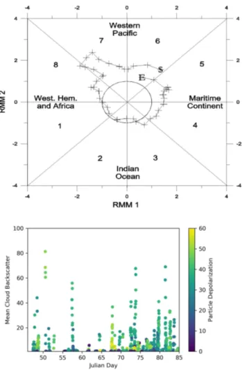
period of the Madden-Julian Oscillation (MJO), the eastward moving disturbance of clouds, rainfall, winds, and pressure that traverses the tropics in 30 to 60 days on average. The upper panel of figure 1 reports the MJO phase diagram during the 50 days of the campaign. We remind that such diagrams represent the magnitude of the first two empirical orthogonal functions of the combined fields of near-equatorially averaged 850-hPa zonal wind, 200-hPa zonal wind, and satellite-observed outgoing longwave radiation (OLR) data (Wheeler and Hendon, 2004). Points representing sequential days are joined by a line, and their
225
distance from the origin is related to the strength of MJO cycle. Their position with respect to the eight quadrants into which the diagram is divided indicates the geographical region in which the MJO phase brings an increase in convection. Labels S and E on the diagram marks the days of beginning and end of our field campaign. According to that, we should have expected an enhanced convection in the second half of the campaign.
Clouds were observed throughout the campaign, with a prevalence in the second part as depicted in the lower panel of figure
230
2 , where a time serie of clouds observation is reported; each point represent the average of BR within clouds on a 3 hours time window. Colour codes the same average for the particle depolarization.
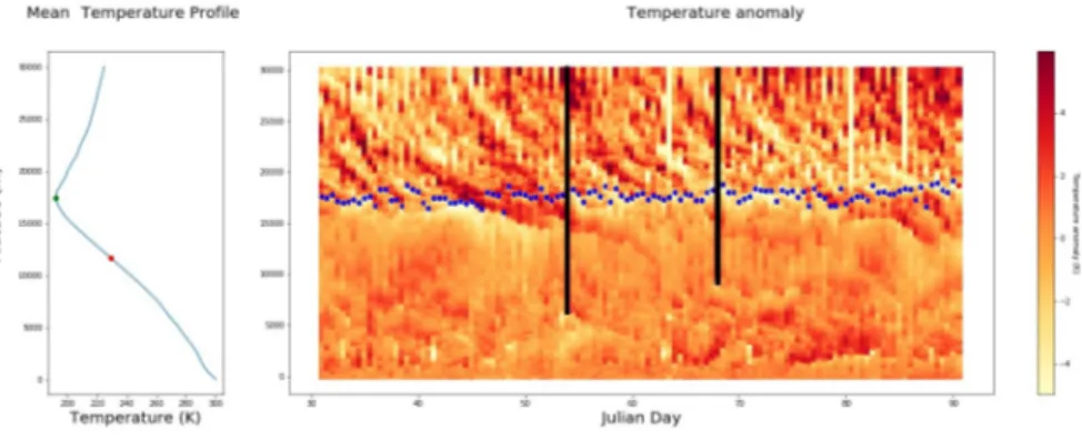
Figure 2 reports the average vertical temperature profile (left panel) during the campaign time frame. On average, the Cold Point Tropopause (CPT) temperature is 192 K at 17400 m at 382 K potential temperature on average; that altitude is nearly coincident with the Lapse Rate Tropopause (LRT) , defined as the level at which the lapse rate becomes less than 2 K/km
235
and the average lapse rate is less than 2 K/km for 2 km above this level, The Level of Neutral Buoyancy (LNB), which we consider to be the one at which the potential temperature equals the equivalent potential temperature at the ground, is at 11600 m at 348K potential temperature on average. In our case it can be shown that this level coincides with the Level of Minimum Stability (LMS), where the vertical gradient of the potential temperature attains a minimum, and thus can be taken as the lower boundary of the TTL (Sunilkumar et al., 2017).
240
On the left panel of the figure the time series of temperature anomaly profiles observed during the campaign are reported. The altitudes of the CPT (blue dots) are also displayed. The pronounced wave-fronts in the stratosphere that are seen to descend from the stratosphere and sometimes penetrating below the CPT are the result of large scale tropical wave activity. We can see here how the structure and variability of the TTL are greatly affected by these fluctuations induced by such gravity waves or Kelvin waves, that influence tropopause height, temperature, cloud occurrence, (Fueglistaler et al., 2009).
245
Prevalent winds were from East, veering South with altitude and becoming southerly close to the Tropopause. 3.2 Clouds vertical distribution and morphology
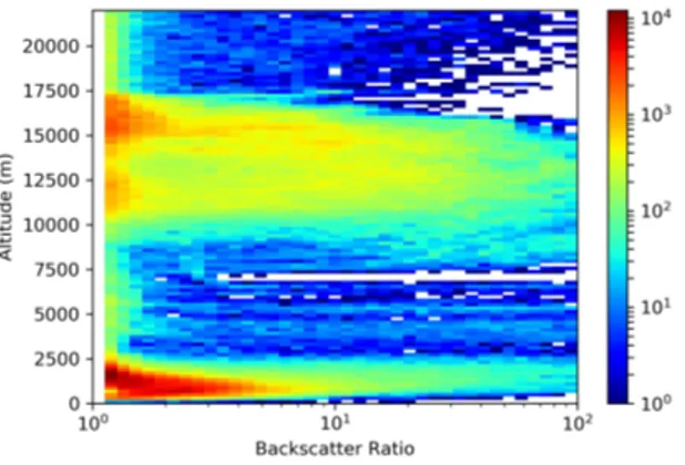
Figure 3 reports the distribution of BR > 1.15 observations with respect to altitude. Each observation is a 5-min average over an altitude interval of 30 m. Low level clouds top extends up to 2.5 km, then a relatively clear altitude range is observed. High
altitude clouds, which are the ones we will focus our attention on, appear from 10 km upward, with two peaks of maximum
250
occurrence respectively at 12 km and at 15 km; then their occurrence tapers off until the tropopause is reached.
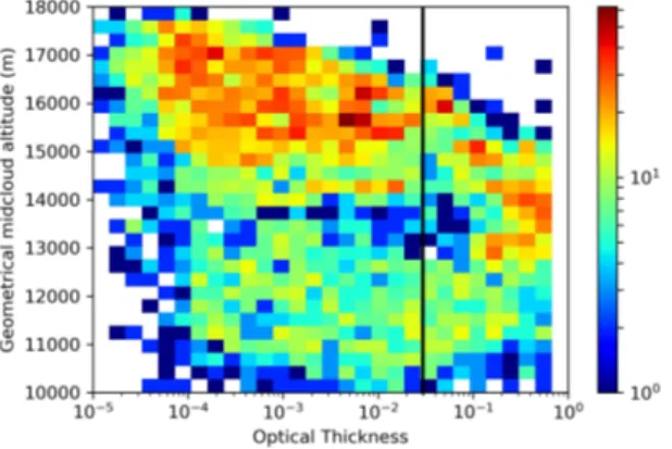
Figure 4 reports the statistics of cloud optical thickness versus geometrical mid cloud altitude. Here and in the figures that follow, the reported data are from 5 min averages of lidar vertical profiles with 30 m vertical resolution, and a cloud is defined as an altitude interval not thinner than 150 m where the condition BR>1.15 is continuously met. The continuous horizontal lines indicate the τ value that separates altostratus and thin cirrus from subvisible cirrus (τ < 0.03). Most of our observations
255
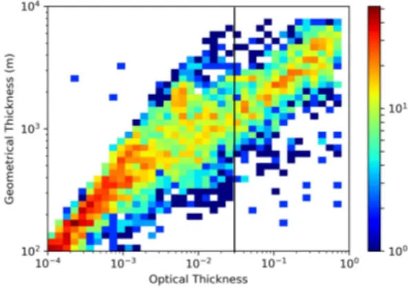
are SVC, mainly collected between 15 km and the Tropopause; the distribution of the SVC has a second maximum in the lower part of the TTL, between 11 and 13 km altitude. The thin cirrus clouds are distributed more evenly in altitudes up to 15 km, with a slight tendency to get thicker with increasing altitude; no significantly thick cirrus are present at the Tropopause. In figure 5 the statistics of τ vs the geometrical cloud thickness ∆z are shown. In spite of the wide spread of the data, an almost linear increase of τ with ∆z is apparent, with two different slopes respectively for the SVC and the thin cirrus classes. Figure
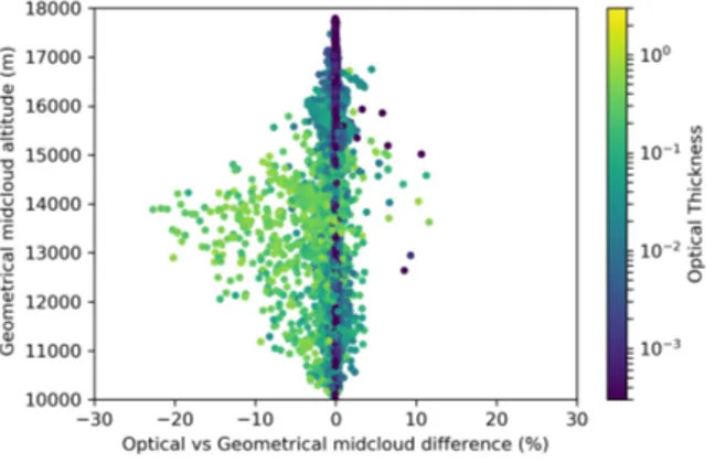
260
6 reports the relative difference between the geometrical and optical mid cloud altitude (zg-zo)/zg, vs altitude, colour coded with τ. Positive values indicate that the backscattering is more intense in the upper part of the cloud, which is then radiatively more effective than the lower part. This parameter may vary depending on the distribution of Ice Water Content (IWC) inside the cloud, in turn affected by the microphysics of particle formation and redistribution by sedimentation and evaporation. In our case, the lower and upper parts of the cirrus appear to produce the same scattering effect for small to medium values of τ,
265
indicative of an even distribution of backscatter inside, which we may take as a proxy for the distribution of IWC. Conversely, the thickest clouds tend to have lower backscatter in their bottom part with respect to the top part, with few exceptions for the highest ones; this is arguably due to mass redistribution by sedimentation and subsequent evaporation.
3.3 Clouds optical properties
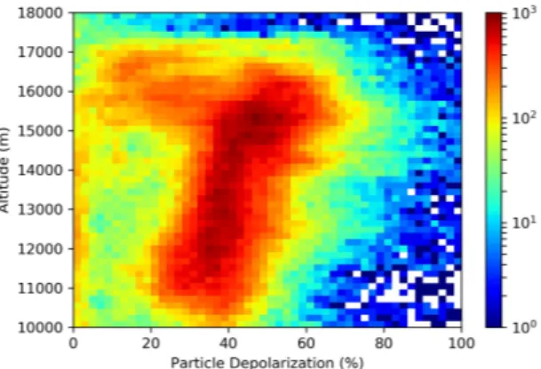
The trend of depolarization with the altitude, i.e. with decreasing temperature, shows a compact linear relationship with a
270
progressive increase towards higher altitudes, as shown in figure 7. This linearity is apparent from 10 km to slightly below the tropopause. It is interesting to note that approaching the tropopause, a different behavious sets in, so that between 15 and 17 km an entire range of depolarization values is also observed. It is possible to show that the data associated with the compact linear increase of depolarization toward higher altitude are associated with particle backscatter coefficients βa covering the entire range of their variability (in our data, between 10−8and 10−4m−1sr−1). Conversely, those depolarization data at high altitude
275
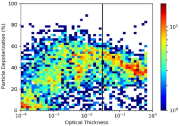
which are almost evenly distributed between 10 and 60%, are associated only with medium to low values of βa. The fact that different optical typologies of clouds coexist in the upper part of the TTL can be drawn also from the inspection of the relation between average particle depolarization δa and optical thickness τ, shown in figure 8. There, two branches can be discerned: for medium to high values of τ associated to thin cirrus, those arguably topping at 15 km in figure 4, there is a decreasing trend of δa vs τ, while for small to medium values of τ associated to SVC, the particle depolarization is more spread through
280
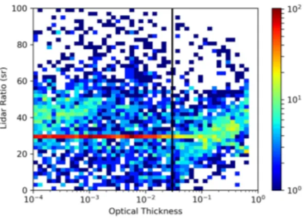
its variability range. The analysis of the LR adds another piece of information, as it is a parameter linked to the average size dimension of the particles: the lower the LR, the larger the particles. In figure 9 we report the occurrence of LR vs τ. For thin clouds LR stays around the value of 29 sr, often measured and reported in literature while for optical thickness typical of SVC,
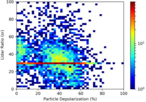
LR tends to get to higher values, suggesting the presence of smaller particles in the clouds. A similar lesson can be learned by looking at the histogram of occurrence of LR and depolarization, shown in figure 10. There, the LR values around 29 sr,
285
typical of thin cirrus, are associated with depolarization significantly higher than those associated with LR around 40 sr, which in the previous figure were linked to optical thickness typical of SVCs. A similar spread in LR has been reported elsewhere: for instance, from one year of cirrus obsservation in the Amazonian basin, Gouveia et al. (2017) report how the most frequent LR were between 18 and 28 sr, peaking at 25 sr for opaque cirrus and at about 21 sr for thin cirrus, and showing a bimodality for SVC with two peaks respectively at 15 sr and at 44 sr. Our observations of clouds with LR around 40 sr are found mainly in the
290
highest part of the TTL at colder temperatures, as shown in figure 11 where LR is reported in relation to the cloud temperature. So in the upper part of the TTL, two classes of clouds are present, namely thin cirrus with high depolarization and low LR, and SVC with medium to low depolarization and larger LR. The optical parameters that we used to discern these two cirrus classes are indicative of differences in the average shape and dimension of the particles that compose them.
3.4 Clouds close to the tropopause
295
It is worthwhile zooming in on what happens close to the Tropopause, therefore we move to a reference system centered at the altitude of the CPT, and we replot the statistics of the particle depolarization data with respect to the distance from the CPT in figure 12; again we are able to see the presence of two modes in the depolarization, paricularly evident from 2 to 1 km below the tropopause, and around the tropopause, one with high values and one with medium to low values of the depolarization. It is worth noting that clouds, especially those with medium to low depolarization values, do not extend significantly above
300
the CPT. In figure 13 for the same subset of observations depicted in figure 12, we report the statistics of the simultaneous occurrence of particle depolarization and local temperature anomalies, these latter calculated as deviations of the temperature profile measured by the concomitant radiosounding with respect to the average temperature profile during the campaign, as reported in the right panel of figure 2. It is evident that cloud occurrence is associated with cold temperature anomalies. It is noteworthy that clouds with high depolarization are present throughout the whole variability range of cold anomalies, while
305
those with medium to low depolarization occur only when the temperature drops 2 to 3 K below the average. It can be shown that such correlation between cloud occurrence and negative temperature anomaly is not present for clouds at lower levels. 4 Trajectory analysis
The trajectory analysis allows possible linking of the optical characteristics of the clouds with the thermal and convective history of the airmass. Clusters of 1000 trajectories were launched backward from the altitude and time of the clouds
obser-310
vations, and the averaged trajectory over each cluster, together with its dispersion, was used for further analysis. Along each of the averaged backtrajectories, the minimum temperature encountered Tminand the time elapsed since that, t(Tmin), was computed, together with the derivatives of temperature dT/dt, potential temperature dθ/dt and pressure dp/dt at the time of lidar measurements, computed as averages over the past 18 hours. Moreover, the following quantities were also computed: the time during which the air mass remained below the temperature attained at the lidar observation t(T (t) < T0); the minimum
potential temperature θminand the maximum pressure pmaxand the relative times elapsed from the lidar observation t(θmin) and t(pmin).
For each averaged backtrajectory, the ‘convective fraction’ - defined as the percentage of the trajectories in the cluster that had met convection - was also computed. The time elapsed since the most probable convection encounter was defined as the time from the maximum increase of the convective fraction in the cluster.
320
This information obtained from the analysis of the retro-trajectory was connected to the measured optical parameters: depo-larization, optical thickness and LR. We give here a brief resume of the main results; a more extensive analysis and supporting figures are available in the supplementary material.
Most of the clouds in the upper part of the TTL are stationary or experience a slight warming, while some of those in the lower part, especially among the thickest ones, are cooling (figures S4, S5 and S6 in Supplementary material).
325
Most of the cloud observations had max temperature differences along the backtrajectories which are below 5 K, with few exceptions for clouds in the mid TTL between 12 and 15 km, with medium to high optical thickness and medium to low depolarization, which experienced temperature differences as large as a few tens of Kelvin (figures S1, S2 and S3 in Supplementary material).
Most of the clouds encountered their minimum temperature Tmin less than 48 hrs before observations therefore relatively
330
recently, with few exceptions of clouds below 14 km, with high optical thickness and medium to low depolarization for which the temporal distance from the minimum of temperature along the backtrajectory was as large as 100-200 hours (figures S13, S14 and S15 in Supplementary material).
Generally, the clouds spent less than 48 hrs below the temperature T0, so indicative of relatively recent origin, with the exception of some clouds present both in the upper part of the TTL, and below 14 km, which spent several days below T0
335
(figures S16, S17 and S18 in Supplementary material).
A more interesting picture came from the analysis of the maximum potential temperature difference along the trajectory, indicative of the altitude jump: while for clouds below 16 km this difference is smaller than 10 K, above that level θmax−θmin is consistently greater, ranging from 15 to 25 K (figure S19, S20 and S21 in Supplementary material). In fact, above that altitude the potential temperature gradient begins to assume stratospheric characteristics. Moreover, the clouds in the TTL and
340
particularly in its upper part had met θminseveral days before the observation,while on the contrary, in the backtrajectories from clouds at lower levels θminwas temporally significantly closer to the observations, going back to some hours up to one or two days before (figures S22, S23 and S24 in Supplementary material).
The convective influence on the cloud airmass spans between 20 and 60 % , evenly spread across altitude, somewhat larger for the highest and optically thinnest clouds (figures S28, S29 and S30 in Supplementary material); the time elapsed from the
345
most likely convective encounter is very often below two days, except for very few cases, scattered throughout the altitude range, when it is greater (figure S31, S32 and S33 in Supplementary material).
It is worthwhile noting that, for the set of high level SVC with low optical thickness and depolarization and high LR which may be depicted on the left side of figures 9 and 10, they have the highest potential temperature difference along the backtrajectory (figures S19, S20 and S21 in Supplementary material), and the longest time interval from θmin(figures S22, S23
and S24 in Supplementary material) and below T0(figures S16, S17 and S18 in Supplementary material), possibly suggesting an origin other than the recent convection one.
5 Discussion
The analysis shows how clouds occurrence extends throughout the whole TTL, with two peaks, one at 10-13 km and the other at or slightly below the CPT; clouds do not extend significantly above it. It is noteworthy how only those upper TTL clouds are
355
largely affected by local atmospheric temperature anomalies.
Depolarization increases with height and generally decrease with temperature. In the upper part of the TTL, depolarization may vary over a wide range, with some of the highest and thinnest SVC clouds attaining medium to low depolarization and LR greater than those found in other SVC at the same altitude, and in thicker clouds below. In situ measurements, reviewed in Lawson et al. (2019), have shown that particle shapes in fresh anvil outflows are markedly different from those in in situ formed
360
cirrus, the latter showing a prevalence of bullet rosettes and polycrystals, virtually absent in the convective cirrus dominated by single crystals and aggregates of crystals: plates, double plates, columns, and irregulars, with some needles, stellars, and dendrites. This difference reflects different formation mechanisms, as ice may form in convective updrafts prior to reaching the homogeneous freezing level (-38◦C). Cirrus from aged outflows have intermediate characteristics. Moreover, in the upper part of the TTL where in situ formation is likely predominant, measurements show in SVC the prevalence of small quasi-spheroids
365
and plates, in concentrations of 1-10 cm−3, while in the lower part of TTL where cirrus can more likely be generated by convection, particles are bigger and attain lower concentrations.
Some of the observed SVC may have had rather long life times, and are associated with negligible lifting in the hours preceding the observation. The study of the convective influence is not conclusive, so we may speculate that this class of SVC may have originated by in situ formation, with nucleation processes that induce morphologies, sizes and concentration of ice
370
crystals that differs from those that we can observe at lower altitudes (11-14 km), where the depolarization and the optical thickness is higher and the LR is lower. Such in situ formation may be triggered by the activity of tropical waves that may induce temperature anomalies as large as 2-3 K close to the CPT, while the clouds in the lower part of the TTL, more likely originated by convective events, are dependent on local temperature conditions only for their subsistence and not for their formation.
375
6 Conclusions
Five weeks of night lidar observations of of equatorial cirrus clouds have been presented and their morphology and optical and geometrical characteristics have been discussed, also in the light of a trajectory analysis aiming at connecting their properties with the thermal and convective history. The lidar-derived depolarization shows a linear increase with altitude up to the top of the troposphere, where a full range of depolarization values is present. For a subset of these high altitude clouds, low
380
of recent significative uplifting in the histories of those airmass suggests a mechanism of formation by in situ condensation, triggered by temperature fluctuation. The fact that the presence of small particles in cirrus particle size distribution increase in percentage with decreasing temperature i.e increasing altitude, and with increasing time since convective influence, has been reported by Woods et al. (2018).
385
Conversely, the majority of cirrus in the TTL have thermal and convective histories compatible with formation from convec-tive outflows, bringing up moisture and ice. In the thickest of them, the negaconvec-tive difference between the optical and geometrical mid cloud altitude gives a hint that larger ice crystals are being removed from the TTL by sedimentation, leaving smaller particles on optically thinner cirrus that can survive for several hours. Compared to observations in other climatically impor-tant regions, observations of equatorial cirrus in the TWP are scarse so this work, albeit limited to lidar observations during a
390
relatively short time frame, contributes to enriching observations. The work would have benefitted from the simultaneous use of balloon hygrometers to better explore the effect of cirrus clouds on the distribution of water vapor in the TTL. An observa-tional campaign with balloon hygrometers and the deployment of the more performing lidar COMCAL by the Alfred Wegener Institute will help to better define the morphology and microphysical processes in TTL in this region.
Data availability. Lidar data are temporarily available at https://stratoclim.icg.kfa-juelich.de/AfcMain/CampaignDataBase/DataMicro, they
395
will migrate to a definitive database in the future. Contact the first author for further information.
Author contributions. FC, MDM, MS, LDL, set up and extensively tested the system and software; FC, MDM deployed and maintained the system in campaign; FC and AS performed the data analysis; SB, BL, AK, provided bactrajectories and convective analysis; SG did a preliminary study on backtrajectory during his master thesis; FC wrote the manuscript which was reviewed by everyone; the software for analysis was produced by FC, MS, LDL, AS, SB.
400
Competing interests. The authors declare that they have no conflict of interest.
Acknowledgements. This study is funded by the StratoClim project by the European Union Seventh Framework Programme under grant agreement no. 603557. The authors gratefully aknowledge the support of Justus Notholt, Institute of Environmental Physics, University of Bremen and Katrin Müller, Alfred Wegener Institute, Potsdam that organized and guided the activities of the Atmospheric Observatory in Palau; Sharon Patris, Coral Reef Research Foundation and Patrick Tellei, Palau Community College, Palau, and Ingo Beninga and Wilfried
405
Ruhe, Impres GmbH, Bremen, which very much assisted us remotely and on the field; finally Maurizio Viterbini, ISAC-CNR now retired without whose invaluable technical support this work would not have been possible.
References
Biavati, G., Di Donfrancesco, G., Cairo, F., and Feist, D. G.: Correction scheme for close-range lidar returns, Applied optics, 50, 5872–5882, 2011.
410
Bissonnette, L. R.: Lidar and multiple scattering, in: Lidar, pp. 43–103, Springer, 2005.
Boehm, M. T. and Verlinde, J.: Stratospheric influence on upper tropospheric tropical cirrus, Geophysical research letters, 27, 3209–3212, 2000.
Bucci, S., Cristofanelli, P., Decesari, S., Marinoni, A., Sandrini, S., Größ, J., Wiedensohler, A., Di Marco, C. F., Nemitz, E., Cairo, F., Di Liberto, L., and Fierli, F.: Vertical distribution of aerosol optical properties in the Po Valley during the 2012 summer campaigns,
415
Atmospheric Chemistry and Physics, 18, 5371–5389, https://doi.org/10.5194/acp-18-5371-2018, https://acp.copernicus.org/articles/18/ 5371/2018/, 2018.
Bucci, S., Legras, B., Sellitto, P., D’Amato, F., Viciani, S., Montori, A., Chiarugi, A., Ravegnani, F., Ulanovsky, A., Cairo, F., and Stroh, F.: Deep convective influence on the UTLS composition in the Asian Monsoon Anticyclone region: 2017 StratoClim campaign results, Atmo-spheric Chemistry and Physics Discussions, 2020, 1–29, https://doi.org/10.5194/acp-2019-1053, https://www.atmos-chem-phys-discuss.
420
net/acp-2019-1053/, 2020.
Cairo, F., Donfrancesco, G. D., Adriani, A., Pulvirenti, L., and Fierli, F.: Comparison of various linear depolarization parameters measured by lidar, Appl. Opt., 38, 4425–4432, https://doi.org/10.1364/AO.38.004425, http://ao.osa.org/abstract.cfm?URI=ao-38-21-4425, 1999. Cairo, F., Di Donfrancesco, G., Snels, M., Fierli, F., Viterbini, M., Borrmann, S., and Frey, W.: A comparison of light
backscat-tering and particle size distribution measurements in tropical cirrus clouds, Atmospheric Measurement Techniques, 4, 557–570,
425
https://doi.org/10.5194/amt-4-557-2011, https://www.atmos-meas-tech.net/4/557/2011/, 2011.
Cairo, F., Di Donfrancesco, G., Di Liberto, L., and Viterbini, M.: The RAMNI airborne lidar for cloud and aerosol research, Atmo-spheric Measurement Techniques, 5, 1779–1792, https://doi.org/10.5194/amt-5-1779-2012, https://amt.copernicus.org/articles/5/1779/ 2012/, 2012.
Cavalieri, O., Cairo, F., Fierli, F., Di Donfrancesco, G., Snels, M., Viterbini, M., Cardillo, F., Chatenet, B., Formenti, P., Marticorena, B.,
430
et al.: Variability of aerosol vertical distribution in the Sahel., Atmospheric Chemistry & Physics Discussions, 10, 2010.
Cavalieri, O., Di Donfrancesco, G., Cairo, F., Fierli, F., Snels, M., Viterbini, M., Cardillo, F., Chatenet, B., Formenti, P., Marticorena, B., et al.: The AMMA MULID network for aerosol characterization in West Africa, International journal of remote sensing, 32, 5485–5504, 2011.
Chen, W.-N., Chiang, C.-W., and Nee, J.-B.: Lidar ratio and depolarization ratio for cirrus clouds, Appl. Opt., 41, 6470–6476,
435
https://doi.org/10.1364/AO.41.006470, http://ao.osa.org/abstract.cfm?URI=ao-41-30-6470, 2002.
Collis, R. and Russell, P.: Lidar measurement of particles and gases by elastic backscattering and differential absorption, in: Laser monitoring of the atmosphere, pp. 71–151, Springer, 1976.
Comstock, J. M. and Jakob, C.: Evaluation of tropical cirrus cloud properties derived from ECMWF model output and ground based mea-surements over Nauru Island, Geophysical Research Letters, 31, https://doi.org/10.1029/2004GL019539, https://agupubs.onlinelibrary.
440
wiley.com/doi/abs/10.1029/2004GL019539, 2004.
Comstock, J. M., Ackerman, T. P., and Mace, G. G.: Ground-based lidar and radar remote sensing of tropical cirrus clouds at Nauru Island: Cloud statistics and radiative impacts, Journal of Geophysical Research: Atmospheres, 107, AAC–16, 2002.
Dawson, K., Meskhidze, N., Josset, D., and Gassó, S.: Spaceborne observations of the lidar ratio of marine aerosols., Atmospheric Chemistry & Physics, 15, 2015.
445
De Deckker, P.: The Indo-Pacific Warm Pool: critical to world oceanography and world climate, Geoscience Letters, 3, 1–12, 2016. Del Guasta, M.: Simulation of LIDAR returns from pristine and deformed hexagonal ice prisms in cold cirrus by means of “face
tracing”, Journal of Geophysical Research: Atmospheres, 106, 12 589–12 602, https://doi.org/10.1029/2000JD900724, https://agupubs. onlinelibrary.wiley.com/doi/abs/10.1029/2000JD900724, 2001.
Dessler, A. and Yang, P.: The distribution of tropical thin cirrus clouds inferred from Terra MODIS data, Journal of climate, 16, 1241–1247,
450
2003.
Di Liberto, L., Angelini, F., Pietroni, I., Cairo, F., Di Donfrancesco, G., Viola, A., Argentini, S., Fierli, F., Gobbi, G., Maturilli, M., et al.: Estimate of the arctic convective boundary layer height from lidar observations: a case study, Advances in Meteorology, 2012, 2012. Donovan, D., Whiteway, J., and Carswell, A. I.: Correction for nonlinear photon-counting effects in lidar systems, Applied optics, 32, 6742–
6753, 1993.
455
Flury, T., wu, D., and Read, W.: Correlation among cirrus ice content, water vapor and temperature in the TTL as observed by CALIPSO and Aura/MLS, Atmospheric Chemistry and Physics Discussions, 11, 25 037–25 061, https://doi.org/10.5194/acpd-11-25037-2011, 2011. Fu, Q., Smith, M., and Yang, Q.: The Impact of Cloud Radiative Effects on the Tropical Tropopause Layer Temperatures, Atmosphere, 9,
https://doi.org/10.3390/atmos9100377, https://www.mdpi.com/2073-4433/9/10/377, 2018.
Fueglistaler, S., Dessler, A., Dunkerton, T., Folkins, I., Fu, Q., and Mote, P. W.: Tropical tropopause layer, Reviews of Geophysics, 47, 2009.
460
Fujiwara, M., Iwasaki, S., Shimizu, A., Inai, Y., Shiotani, M., Hasebe, F., Matsui, I., Sugimoto, N., Okamoto, H., Nishi, N., Hamada, A., Sakazaki, T., and Yoneyama, K.: Cirrus observations in the tropical tropopause layer over the western Pacific, Journal of Geo-physical Research: Atmospheres, 114, https://doi.org/10.1029/2008JD011040, https://agupubs.onlinelibrary.wiley.com/doi/abs/10.1029/ 2008JD011040, 2009.
Garrett, T., Heymsfield, A., McGill, M. J., Ridley, B., Baumgardner, D., Bui, T., and Webster, C.: Convective generation of cirrus near the
465
tropopause, Journal of Geophysical Research: Atmospheres, 109, 2004.
Gouveia, D. A., Barja, B., Barbosa, H. M. J., Seifert, P., Baars, H., Pauliquevis, T., and Artaxo, P.: Optical and geometrical properties of cirrus clouds in Amazonia derived from 1 year of ground-based lidar measurements, Atmospheric Chemistry and Physics, 17, 3619–3636, https://doi.org/10.5194/acp-17-3619-2017, https://www.atmos-chem-phys.net/17/3619/2017/, 2017.
Heymsfield, A. J., McFarquhar, G. M., Collins, W. D., Goldstein, J. A., Valero, F., Spinhirne, J., Hart, W., and Pilewskie, P.: Cloud properties
470
leading to highly reflective tropical cirrus: Interpretations from CEPEX, TOGA COARE, and Kwajalein, Marshall Islands, Journal of Geophysical Research: Atmospheres, 103, 8805–8812, 1998.
Immler, F., Krüger, K., Fujiwara, M., Verver, G., Rex, M., and Schrems, O.: Correlation between equatorial Kelvin waves and the occurrence of extremely thin ice clouds at the tropical tropopause, Atmospheric Chemistry and Physics, 8, 4019–4026, https://doi.org/10.5194/acp-8-4019-2008, https://www.atmos-chem-phys.net/8/4019/2008/, 2008.
475
Jensen, E. J., Toon, O. B., Pfister, L., and Selkirk, H. B.: Dehydration of the upper troposphere and lower stratosphere by subvisible cirrus clouds near the tropical tropopause, Geophysical Research Letters, 23, 825–828, https://doi.org/10.1029/96GL00722, https://agupubs. onlinelibrary.wiley.com/doi/abs/10.1029/96GL00722, 1996.
Kar, J., Vaughan, M. A., Lee, K.-P., Tackett, J. L., Avery, M. A., Garnier, A., Getzewich, B. J., Hunt, W. H., Josset, D., Liu, Z., Lucker, P. L., Magill, B., Omar, A. H., Pelon, J., Rogers, R. R., Toth, T. D., Trepte, C. R., Vernier, J.-P., Winker, D. M., and Young, S. A.: CALIPSO lidar
calibration at 532 nm: version 4 nighttime algorithm, Atmospheric Measurement Techniques, 11, 1459–1479, https://doi.org/10.5194/amt-11-1459-2018, https://www.atmos-meas-tech.net/11/1459/2018/, 2018.
Klett, J. D.: Lidar inversion with variable backscatter/extinction ratios, Applied optics, 24, 1638–1643, 1985.
Knapp, K. R., Ansari, S., Bain, C. L., Bourassa, M. A., Dickinson, M. J., Funk, C., Helms, C. N., Hennon, C. C., Holmes, C. D., Huffman, G. J., et al.: Globally gridded satellite observations for climate studies, Bulletin of the American Meteorological Society, 92, 893–907,
485
2011.
Kremser, S., Wohltmann, I., Rex, M., Langematz, U., Dameris, M., and Kunze, M.: Water vapour transport in the tropical tropopause region in coupled Chemistry-Climate Models and ERA-40 reanalysis data., Atmospheric Chemistry & Physics, 9, 2009.
Krämer, M., Rolf, C., Luebke, A., Afchine, A., Spelten, N., Costa, A., Zoeger, M., Smith, J., Herman, R., Buchholz, B., Ebert, V., Baum-gardner, D., Borrmann, S., Klingebiel, M., and Avallone, L.: A microphysics guide to cirrus clouds – Part 1: Cirrus types, Atmospheric
490
Chemistry and Physics Discussions, 15, 31 537–31 586, https://doi.org/10.5194/acpd-15-31537-2015, 2015.
Kubota, H., Shirooka, R., Ushiyama, T., Chuda, T., Iwasaki, S., and Takeuchi, K.: Seasonal Variations of Precipitation Properties Associated with the Monsoon over Palau in the Western Pacific, Journal of Hydrometeorology, 6, 518–531, https://doi.org/10.1175/JHM432.1, https: //doi.org/10.1175/JHM432.1, 2005.
Lawson, R. P., Woods, S., Jensen, E., Erfani, E., Gurganus, C., Gallagher, M., Connolly, P., Whiteway, J., Baran, A. J., May, P., Heymsfield,
495
A., Schmitt, C. G., McFarquhar, G., Um, J., Protat, A., Bailey, M., Lance, S., Muehlbauer, A., Stith, J., Korolev, A., Toon, O. B., and Krämer, M.: A Review of Ice Particle Shapes in Cirrus formed In Situ and in Anvils, Journal of Geophysical Research: Atmospheres, 124, 10 049–10 090, https://doi.org/10.1029/2018JD030122, https://agupubs.onlinelibrary.wiley.com/doi/abs/10.1029/2018JD030122, 2019. Legras, B. and Bucci, S.: Confinement of air in the Asian monsoon anticyclone and pathways of convective air to the stratosphere
during summer season, Atmospheric Chemistry and Physics Discussions, 2019, 1–37, https://doi.org/10.5194/acp-2019-1075, https:
500
//www.atmos-chem-phys-discuss.net/acp-2019-1075/, 2019.
Nee, J., Lien, C., Chen, W., and Lin, C.: Lidar detection of cirrus cloud in Chung-Li (25 N, 121 E), J. Atmos. Sci, 55, 2249–2257, 1998. O’Connor, E. J., Illingworth, A. J., and Hogan, R. J.: A Technique for Autocalibration of Cloud Lidar, Journal of Atmospheric
and Oceanic Technology, 21, 777–786, https://doi.org/10.1175/1520-0426(2004)021<0777:ATFAOC>2.0.CO;2, https://doi.org/10.1175/ 1520-0426(2004)021<0777:ATFAOC>2.0.CO;2, 2004.
505
Pace, G., Cacciani, M., di Sarra, A., Fiocco, G., and Fuà, D.: Lidar observations of equatorial cirrus clouds at Mahé Seychelles, Journal of Geophysical Research: Atmospheres, 108, 2003.
Papagiannopoulos, N., Mona, L., Alados-Arboledas, L., Amiridis, V., Baars, H., Binietoglou, I., Bor-toli, D., D’Amico, G., Giunta, A., Guerrero-Rascado, J. L., Schwarz, A., Pereira, S., Spinelli, N., Wandinger, U., Wang, X., and Pappalardo, G.: CALIPSO climatological products: evaluation and suggestions
510
from EARLINET, Atmospheric Chemistry and Physics, 16, 2341–2357, https://doi.org/10.5194/acp-16-2341-2016, https: //acp.copernicus.org/articles/16/2341/2016/, 2016.
Pfister, L., Selkirk, H. B., Jensen, E. J., Schoeberl, M. R., Toon, O. B., Browell, E. V., Grant, W. B., Gary, B., Mahoney, M. J., Bui, T. V., and Hintsa, E.: Aircraft observations of thin cirrus clouds near the tropical tropopause, Journal of Geophysical Research: Atmospheres, 106, 9765–9786, https://doi.org/10.1029/2000JD900648, https://agupubs.onlinelibrary.wiley.com/doi/abs/10.1029/2000JD900648, 2001.
515
Pisso, I. and Legras, B.: Turbulent vertical diffusivity in the sub-tropical stratosphere, Atmospheric Chemistry and Physics, 8, 697–707, https://doi.org/10.5194/acp-8-697-2008, https://www.atmos-chem-phys.net/8/697/2008/, 2008.
Platt, C., Young, S., Manson, P., Patterson, G., Marsden, S., Austin, R., and Churnside, J.: The optical properties of equatorial cirrus from observations in the ARM pilot radiation observation experiment, Journal of the Atmospheric Sciences, 55, 1977–1996, 1998.
Platt, C., Young, S., Austin, R., Patterson, G., Mitchell, D., and Miller, S.: LIRAD observations of tropical cirrus clouds in MCTEX. Part I:
520
Optical properties and detection of small particles in cold cirrus, Journal of the atmospheric sciences, 59, 3145–3162, 2002.
Platt, C. M. R., Scott, S. C., and Dilley, A. C.: Remote Sounding of High Clouds. Part VI: Optical Properties of Midlatitude and Tropical Cirrus, Journal of the Atmospheric Sciences, 44, 729–747, https://doi.org/10.1175/1520-0469(1987)044<0729:RSOHCP>2.0.CO;2, https: //doi.org/10.1175/1520-0469(1987)044<0729:RSOHCP>2.0.CO;2, 1987.
Prabhakara, C., Kratz, D., Yoo, J.-M., Dalu, G., and Vernekar, A.: Optically thin cirrus clouds: Radiative impact on the warm pool, Journal
525
of Quantitative Spectroscopy and Radiative Transfer, 49, 467–483, 1993.
Ramanathan, V. and Collins, W.: Thermodynamic regulation of ocean warming by cirrus clouds deduced from observations of the 1987 El Nino, Nature, 351, 27–32, 1991.
Reichardt, J., Reichardt, S., Hess, M., and McGee, T. J.: Correlations among the optical properties of cirrus-cloud particles: Microphysical interpretation, Journal of Geophysical Research: Atmospheres, 107, AAC 8–1–AAC 8–12, https://doi.org/10.1029/2002JD002589, https:
530
//agupubs.onlinelibrary.wiley.com/doi/abs/10.1029/2002JD002589, 2002.
Rosati, B., Herrmann, E., Bucci, S., Fierli, F., Cairo, F., Gysel, M., Tillmann, R., Größ, J., Gobbi, G. P., Liberto, L. D., et al.: Studying the vertical aerosol extinction coefficient by comparing in situ airborne data and elastic backscatter lidar, 2016.
Rossow, W. B. and Schiffer, R. A.: Advances in understanding clouds from ISCCP, Bulletin of the American Meteorological Society, 80, 2261–2288, 1999.
535
Sassen, K. and Benson, S.: A midlatitude cirrus cloud climatology from the Facility for Atmospheric Remote Sensing. Part II: Microphysical properties derived from lidar depolarization, Journal of the Atmospheric Sciences, 58, 2103–2112, 2001.
Sassen, K. and Cho, B. S.: Subvisual-Thin Cirrus Lidar Dataset for Satellite Verification and Climatological Research, Journal of Applied Meteorology, 31, 1275–1285, https://doi.org/10.1175/1520-0450(1992)031<1275:STCLDF>2.0.CO;2, https://doi.org/10.1175/ 1520-0450(1992)031<1275:STCLDF>2.0.CO;2, 1992.
540
Sassen, K., Benson, R. P., and Spinhirne, J. D.: Tropical cirrus cloud properties derived from TOGA/COARE airborne polarization lidar, Geophysical research letters, 27, 673–676, 2000.
Snels, M., Cairo, F., Colao, F., and Di Donfrancesco, G.: Calibration method for depolarization lidar measurements, International Journal of Remote Sensing, 30, 5725–5736, 2009.
Spichtinger, P.: Shallow cirrus convection – a source for ice supersaturation, Tellus A: Dynamic Meteorology and Oceanography, 66, 19 937,
545
https://doi.org/10.3402/tellusa.v66.19937, https://doi.org/10.3402/tellusa.v66.19937, 2014.
Stohl, A., Forster, C., Frank, A., Seibert, P., and Wotawa, G.: Technical note: The Lagrangian particle dispersion model FLEXPART version 6.2, Atmospheric Chemistry and Physics, 5, 2461–2474, https://doi.org/10.5194/acp-5-2461-2005, https://www.atmos-chem-phys.net/5/ 2461/2005/, 2005.
Sunilkumar, S. V. and Parameswaran, K.: Temperature dependence of tropical cirrus properties and radiative effects, Journal of
Geo-550
physical Research: Atmospheres, 110, https://doi.org/10.1029/2004JD005426, https://agupubs.onlinelibrary.wiley.com/doi/abs/10.1029/ 2004JD005426, 2005.
Sunilkumar, S. V., Muhsin, M., Venkat Ratnam, M., Parameswaran, K., Krishna Murthy, B. V., and Emmanuel, M.: Boundaries of tropical tropopause layer (TTL): A new perspective based on thermal and stability profiles, Journal of Geophysical Research: Atmospheres, 122, 741–754, https://doi.org/10.1002/2016JD025217, https://agupubs.onlinelibrary.wiley.com/doi/abs/10.1002/2016JD025217, 2017.
Tissier, A.-S. and Legras, B.: Convective sources of trajectories traversing the tropical tropopause layer, Atmospheric Chemistry and Physics, 16, 3383–3398, https://doi.org/10.5194/acp-16-3383-2016, https://www.atmos-chem-phys.net/16/3383/2016/, 2016.
Tzella, A. and Legras, B.: A Lagrangian view of convective sources for transport of air across the Tropical Tropopause Layer: distribu-tion, times and the radiative influence of clouds, Atmospheric Chemistry and Physics, 11, 12 517–12 534, https://doi.org/10.5194/acp-11-12517-2011, https://www.atmos-chem-phys.net/11/12517/2011/, 2011.
560
Uthe, E., EE, U., and PB, R.: LIDAR OBSERVATIONS OF TROPICAL HIGH-ALTITUDE CIRRUS CLOUDS., 1977.
Wang, T. and Dessler, A. E.: Analysis of cirrus in the tropical tropopause layer from CALIPSO and MLS data: A water perspective, Journal of Geophysical Research: Atmospheres, 117, https://doi.org/10.1029/2011JD016442, https://agupubs.onlinelibrary.wiley.com/doi/abs/10. 1029/2011JD016442, 2012.
Wang, T., Wu, D. L., Gong, J., and Tsai, V.: Tropopause Laminar Cirrus and Its Role in the Lower Stratosphere Total Water Budget,
565
Journal of Geophysical Research: Atmospheres, 124, 7034–7052, https://doi.org/10.1029/2018JD029845, https://agupubs.onlinelibrary. wiley.com/doi/abs/10.1029/2018JD029845, 2019.
Weinzierl, B., Sauer, D., Esselborn, M., Petzold, A., Veira, A., Rose, M., Mund, S., Wirth, M., Ansmann, A., Tesche, M., et al.: Microphysical and optical properties of dust and tropical biomass burning aerosol layers in the Cape Verde region—an overview of the airborne in situ and lidar measurements during SAMUM-2, Tellus B: Chemical and Physical Meteorology, 63, 589–618, 2011.
570
Wheeler, M. C. and Hendon, H. H.: An all-season real-time multivariate MJO index: Development of an index for monitoring and prediction, Monthly weather review, 132, 1917–1932, 2004.
Woods, S., Lawson, R. P., Jensen, E., Bui, T. P., Thornberry, T., Rollins, A., Pfister, L., and Avery, M.: Microphysical Properties of Tropical Tropopause Layer Cirrus, Journal of Geophysical Research: Atmospheres, 123, 6053–6069, https://doi.org/10.1029/2017JD028068, https: //agupubs.onlinelibrary.wiley.com/doi/abs/10.1029/2017JD028068, 2018.
575
Young, S. A.: Analysis of lidar backscatter profiles in optically thin clouds, Appl. Opt., 34, 7019–7031, https://doi.org/10.1364/AO.34.007019, http://ao.osa.org/abstract.cfm?URI=ao-34-30-7019, 1995.
Figure 1. Upper panel: Madden-Julian Oscillation phase diagram for the campaign duration. Days of start and ending of the campaign are marked respectively with an S and an E. Data from the Australian Geovernment Bureau of Meteorology (http://www.bom.gov.au/climate/mjo/). Lower panel: Timeseries of observations of clouds Backscatter Ratio (BR) during the campaign. The colour codes the Particle Depolarization. Data points are averages over 300m of the lidar profile and over 3 hrs of observations. Observations with BR<1.15 have not been reported.
Figure 2. Left panel: Average temperature profile during the campaign timeframe. The green dot marks the Cold Point Tropopause (CPT) at 17400m, the red dot marks the Level of Neutral Buoyancy at 11600 m. The Tropical Tropopause Layer (TTL) can be considered to be withint these two limits. Right panel: Temperature anomaly with respect to the average temperature profile on the left. Data are from 12-hrs radiosoundings routinely launched by the Weather Service Office of Palau from Koror, Palau (station 91408) downloaded from: http://weather.uwyo.edu/upperair/sounding.html
Figure 3. Distribution of Backscatter Ratio observatons vs altitude. Data are 5 min averages of lidar vertical profiles, with 30 m vertical resolution. The colour codes the number of samples in each bin. Only data with BR>1.15 have bee reported.
Figure 4. Distribution of cloud optical thickness observations vs mid cloud altitude. The colour codes the number of samples in each bin. The thick black line reports the optical thickness threshold value for SVC.
Figure 5. Distribution of cloud optical vs geometrical thickness. The thick black line reports the optical thickness threshold value for SVC. The colour codes the number of samples in each bin.
Figure 6. Scatterplot of the relative difference between the optical and geometrical mdcloud altitude, vs the geometrical mid cloud altitude, colour coded with the cloud optical thickness.
Figure 8. Distribution of particle depolarization vs optical thickness. The thick black line reports the optical thickness threshold value for SVC.
Figure 9. Distribution of Lidar Ratio (LR) vs optical thickness. The thick black line reports the optical thickness threshold value for SVC. The observations that accumulate along the line at LR=29 sr are those for which the inversion according to Young (1995) did not produce convergence to a result for LR. For these observation, LR was set at 29 sr by default.
Figure 10. Distribution of Lidar Ratio (LR) vs Particle Depolarization. The observations that accumulate along the line at LR=29 sr are those for which the inversion according to Young (1995) did not produce convergence to a result for LR. For these observation, LR was set at 29 sr by default.
Figure 11. Distribution of Lidar Ratio (LR) vs mid cloud Temperature. The observations that accumulate along the line at LR=29 sr are those for which the inversion according to Young (1995) did not produce convergence to a result for LR. For these observation, LR was set at 29 sr by default.
Figure 13. Distribution of particle depolarization observations vs temperature anomaly with respect to the average temperature profile as reported in the left panel of figure 2. Only data from clouds within 2500 m from the CPT are reported.
Table 1. Lidar specifications
Technical specifications of the lidar system
Detected wavelengths 532 nm (two polarizations) Laser type Nd-YAG (SHG 532 nm) Pulse duration 1 ns
Laser repetition rate 1 kHz
Laser output energy 1 mJ at 532 nm Telescope diameter 20 cm
Telescope type F/1.5 Newtonian Telescope field of view 0.7 mrad
Beam divergence 0.4 mrad, full angle Filter bandwidth 2 nm
Vertical resolution From 3.75 to 150m in photoncounting mode From 1.875 to 15m in current mode Vertical range 1024×Vertical resolution
Time resolution down to 1s