DEVELOPMENT AND ANALYSIS OF AN EPIDEMIOLOGICAL INFLUENZA MODEL
by
CECILIA RUTH d'OLIVEIRA
S.B., Massachusetts Institute
(1977)
of Technology
SUBMITTED IN PARTIAL FULFILLMENT OF THE REQUIREMENTS FOR THE
DEGREE OF MASTER OF SCIENCE
at the
MASSACHUSETTS INSTITUTE OF TECHNOLOGY JUNE 1979
Signature of Author... %.. ..--- ,.. ... Alfred P. Sloan Schoo of Management, May 25, 1979
Certified by ... ... ...
Thesis Supervisor
Accepted by...
Archives
Chairman, Department CommitteeMASSACHUSETTS INSTITUTE OF TECHNOLOGY
JUN 2 5 1979
DEVELOPMENT AND ANALYSIS OF A EPIDEMIOLOGICAL INFLUENZA MODEL by
Cecilia Ruth d'Oliveira
Submitted to the Department of the Sloan School of Management on May 25, 1979 in partial fulfillment of the requirements
for the Degree of Master of Science
ABSTRACT
This thesis is an attempt to develop and analyze a computer-based influenza epidemic model that could be used in evaluating the
effects of alternative immunization strategies. The objectives of this
thesis are to present a general mathematical model, to analyze the
sensitivity of the model 's parameters through computer simulation and to indicate how the model might be applied to an anticipated influenza
epidemic. It is hoped that this thesis will present a structure that
will be useful to individuals interested in the control of influenza
epidemics.
The mathematical model that is used is the Kermack-McKendrik deterministic disease model. This model is adapted to influenza based
on epidemiological characteristics of this disease. The computer programs that perform the analysis are written in APL. The model is applied to
the 1957 epidemic of Asian influenza, One of the major limitations of
the model is the assumption of uniform exposure opportunities. THESIS SUPERVISOR: Stan N, Finkelstein
TITLE: Assistant Professor of Management 2
ACKNOWLEDGMENTS
I would like to thank my thesis supervisor, Professor Stan N. Finklestein, and Professor Robert S. Pindyck, for initially posing the problem that developed into this thesis topic, I would also like to
thank each of them for the insights they provided,
To my unofficial thesis partners - the dynamic duo of Andrew Gralla and Charles Smart - I present my thanks for making the hours spent in the computer room not just bearable but fun.
I would especially like to acknowledge my classmates who never failed to respond to my questions or my requests for assistance,
TABLE OF CONTENTS Abstract . . . .. . . . . . Acknowledgments . . . . Table of Contents . , List of Figures . . . . , , . List of Tables... ,, .. SECTIONS 1. Introduction . . .. . .. . .
2. The Epidemiology of Influenza 2.1 General Concepts of Epi 2.2 Epidemic Influenza . , 2.3 The Spread of Influenza 2.4 Immunity to Influenza
2.5 Age Group Differences i
2.6 Unanswered Questions
3. The Disease Model . . . .
3.1 General Epidemic Models
3.2 A Verbal Description , 3.3 The Basic Assumptions . 3.4 The Equations . . . . 3.5 The Parameters . . . , 3.5.1 The Removal Ra 3.5.2 The Initial Im 3,5.3 The Contact Ra demiolo , . , n Morbi nune Po te. . 9 , , , , ,9 ,ad , ,9 gy. , ,9 di ty 9 ,9 . .9 Morta i ty Page 2 3 4 7 9 10 13 13 16 18 20 22 25 27 27 28 30 31 32 32 33 34 pulation, . . , .t . .
3.6 Theoretical Analysis . , . . . . .. , . . . .
3.6.1 The Size of the Epidemic . ..0. . .. . 3.6.2 The Size of the Epidemic Depends on the
Size of the Initial Immune Population
3.6.3 The Size of the Epidemic Depends on the the Relative Contact Rate . . .
, . 41 . . . . . . 42 4. Resul 4.1 4.2 4.3 4.4 4.5 4.6 4.7 4.8 5. Appli 5.1 5.2 5.3 5.4
3.6.4 The Threshold Theorem . . . .
ts of the Computer Model . . . .
The Computer Model . . . .
Sensitivity Analysis . . . .
Sensitivity of the Model to the Contact Rate. . . . Sensitivity of the Model to the Initial Immunes Sensitivity of the Model to the Removal Rate .
Sensitivity of the Model to the Initial Infectives The Impact of a Constant Relative Contact Rate .
The Course of the Epidemic . , .
cation of the Model . . . ... ...--.-. Calibrating the Parameters
Calibration of the Removal Rate . . . . .
Calibration of the Initial Immunes . . , . . . . .
Calibration of the Contact Rate .
5.5 Fitting the Model to a Particular Epidemic . . . . . 5.6 Comparison with Traditional Methods of Analysis
6. Limitations and Suggestions for Future Work . . . .
6.1 Effects of Misspecification of Parameters . .
6.2 Allowing for Multiple Groups in the Population
42 44 44 46 47 51 54 61 63 66 73 73 75 76 77 80 86 88 88 94 - -. -. . . . V
APPENDIX A . .. . . . .. . . . . . 96
APPENDIX B
. .
, .. .. . .. , , , , , , , . , , . . , . 99APPENDIX C . . . ,F , . . .. . . ... ... 118 REFERENCES . .. . . . . . , , , ,t ,t , ,, 130
LIST OF FIGURES
Page The Stages of Infection . . . . . . . . ,. . . .
Figure 2. Frequency of Isolation of Influenza A virus From Patients (in %) According to Day of the Disease Figure 3. Cases Reported (% of the Population) Using the
Equation with Removal Rate of .5 and Variable Contact Rates and Initial Immunes . , . . . . Figure
Figure
Cases Reported (% of the Population) Using the Equation with Removal Rate of .33 and Variable Contact Rates and Initial Immunes . . . . A Three Dimensional View of Sensitivity Analysis
Figure 6. Cases Reported (% of the Population) Using the Computer Model with Removal Rate of .5 and Variable Contact Rates and Initial Immunes Figure 7. New Cases Reported (% of the Population) By Day
of the Epidemic Using the Computer Model with Removal Rate of .5, Initial Immunes of 40% and Variable Contact Rates . . . ,. . .. .
Figure 8.
Figure 9.
Figure 10.
Figure 11.
New Cases Reported (% of the Population) By Day of the Epidemic Using the Computer Model with Removal Rate of .5, Initial Immunes of 30% and Variable Contact Rates . . , , , , , , , , , ,
New Cases Reported (% of the Population) By Day of the Epidemic Using the Computer Model with Removal Rate of .5, Contact Rate of 1 and
Variable Initial Immunes . . . ,
New Cases Reported (% of the Population) By Day of the Epidemic Using the Computer Model with Removal Rate of .5, Contact Rate of 1.25 and Variable Initial Immunes . . . . , , . . . . .
Cases Reported (% of the Population) Using the Computer Model with Contact Rate of .85 and Variable Removal Rates and Initial Immunes .
Figure
Figure 12. Figure 13. Figure 14. Figure 15, Figure 16. Figure 17.
New Cases Reported (% of the Population) By Day of the Epidemic Using the Computer Model with Removal Rate of .5, Contact Rate of .85 and
Initial Immunes of 25% . . . .
Weekly Incidence of Influenza From Week Ending October 5, 1957 to Week Ending November 30, 1957
(as a % of the Total Incidence of the Period) , ,
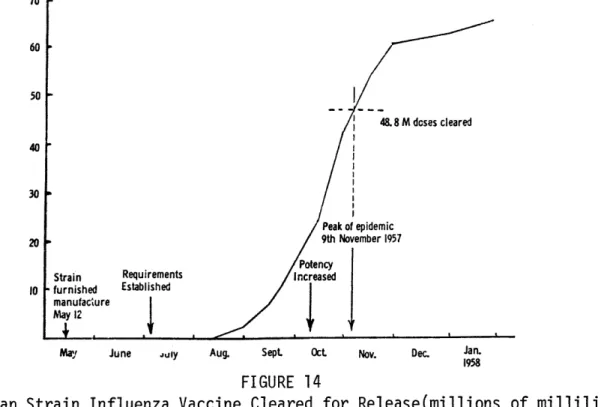
Asian Strain Influenza Vaccine Cleared for Release (Millions of Milliliters) . . . . ... . . .
New Cases Reported (% of the Population) By Day of the Epidemic Using the Computer Model with
Removal Rate of .5, for Three Combinations of Contact Rate and Initial Immunes That Produce Epidemics Resembling the 1957 Asian Epidemic Several Combi-nations of the Contact Rate and Initial Immunes Will Result in a Particular Attack Rate, with the Removal Rate at .5 ,
New Cases Reported (% of the Population) By Day of the Epidemic Using the Computer Model with Removal Rate of .5 for Epidemics with Similar
LIST OF TABLES
Page Table 1. Attack Rates (Per 100) By Age From the
Practice of a London Doctor . . , , , , , , Table 2. Excess Mortality From Influenza and Pneumonia During Sected Influenza Epidemic Years . . ,
Table 3. Distribution
(%)
of Influenza Deaths By Age In England and Wales For Selected Years . , , .Table 4. Attack Rate Calculated with Removal Rate of
.5 and Variable Contact Rates and Initial
Immunes (Calculated from the Equation) . .. .
Table 5. Solution of the Model for Removal Rate of .5, with Varying Contact Rates and Initial Immunes Table 6, Solution of the Model for Contact Rate of ,85,
with Varying Removal Rates and Initial Immunes Table 7. Solution of the Model for Contact Rate of 1,
with Varying Initial Immunes and Infective
Periods of Constant Length , , . , Table 8. Comparison of the Model Results for Contact
Rate of .8, Using Two Different Types of
Infective Period ., .. . . .. .. , ,
Table 9. Solution of the Model as the Initial Infective Population is Varied . . . . . 23 , 24 25 . 38 , 49 , 57 . . Table 10. Table 11. Table 12. Table 13. Table 14. Table 15.
Solution of the Model for Constant Relative Contact Rate of 1,7 and Varying Initial Immunes The Course of the Epidemic for Contact Rate of
.85, Removal Rate of .5, Initial Immunes of 25% and Initial Infectives of .00001% . . .. ..
The Spread of the 1957 Asian Influenza . . . .
Attack Rates Resulting From Various Vaccination Programs with Removal Rate of .5, Contact Rate of .75, Initial Immunes of 10% and Efficacy of 70% Change in Attack Rate for Change in Initial Immunes at an Attack Rate of 36%, for Various Contact
Rate and Initial Immunes Combinations , . , , * . Effects of the Misspecification of Parameters . , ,
INTRODUCTION
This thesis is an attempt to develop and analyze a computer-based influenza epidemic model that could be used in evaluating the effects of alternative immunization strategies. The objectives of this thesis are to present a general mathematical model, to analyze the sensitivity of the model's parameters through computer simulation and to indicate how the model might be applied to an anticipated
influenza epidemic. It is hoped that this thesis will present a structure that will be useful to individuals interested in the control of influenza epidemics.
Mathematical disease models were first developed in the 1920's, prior to the discovery and isolation of the influenza virus in 1933. The
literature abounds with treatises on these and subsequent mathematical disease models.
This thesis extends work done in these models in two ways.
First, there is little written regarding the calibration of the parameters present in these models. This calibration is necessary to apply the models to real world situations. This thesis cannot present a set of parameter values that will apply to all influenza epidemics, Influenza epidemics vary in intensity and other characteristics due to the strain of the virus, the susceptibility of the population and the timing of the epidemic in terms of season. Therefore the model that is presented must be
specified by the decision maker based on information available at the time an epidemic threatens. There is an attempt in this thesis however
to discuss proper ranges for the parameters, as well as how the actual values might be determined given the appropriate information.
The second way that this thesis extends work that has previously been done is in applying the model to influenza rather than to another disease. The few applications of disease models that exist in the literature are primarily concerned with measles, This is probably due to the relatively good understanding we have of measles, Most states and countries require that all cases of measles be reported to local health authorities. Immunity to measles is straightforward in that once an individual is infected he experiences lifetime immunity.
In contrast, influenza suffers from a lack of consistent and reliable information. This is partly due to the imprecision of
the clinical diagnosis of influenza, In fact the best indicator of the presence of the influenza virus is the characteristic epidemic proportions that accompany it. In addition, notification of influenza cases is not usually mandatory by either doctors or individuals.
There is little consensus about how influenza epidemics arise or the nature and duration of the immunity that is acquired after infection.
These aspects of the influenza problem as well as others including the variability of the influenza virus and the periodic antigenic shifts that viruses undergo make influenza very difficult to model.
One of the major advantages that this thesis offers to those interested in evaluating immunization control strategies is the
recognition within the model of the concept of "herd immunity," This refers to the protection that the entire community gains from the vaccination of one of its members. The vaccination of the one member
protects not only that one individual but also the other individuals with whom he might associate.
This thesis will first present the epidemiological factors that must be considered in modeling the spread of a disease, This will include a discussion of general concepts as well as the special
characteristics of influenza.
This background will allow us to present a general epidemic model which is built upon many of the epidemiological concepts. This
presentation will include the assumptions of the model as well as a discussion of the model's parameters. This model will first be analyzed mathematically.
Computer simulation of the epidemic model will allow us to determine the sensitivity of the model to various parameters,
We can then apply the model to a particular epidemic. This will include an intital specification of a "base case" (no vaccination
program in effect) epidemic, which we will define as the 1957 Asian influenza epidemic. After the parameters are specified for this base case we then indicate how alternative strategies may be analyzed.
Finally, we look at particular problems in application and limitations of the model,
THE EPIDEMIOLOGY OF INFLUENZA
In The Mathematical Theory of Epidemics, Bailey states
In many fields of biological science it is possible to pursue the statistical theory of macroscopic processes more or less independently of the "fine structure" involved. To a great extent this is also true of the mathematical theory of epidemics, but itmay well be that as the subject developes, especially where features like incubation periods and the occurrence of clinical symptoms are concerned, more attention will have to be paid to the biological details than is envisaged here.
We find that in order to build a general, non-specific disease model we must understand certain general principles of
epidem-iology, These principles provide a framework for the design. At the point where we want to apply a general disease model to a specific disease we must understand the biological details of the disease,
This section will attempt to present both the general principles of epidemiology which are the backbone of the model, as well as the specific characteristics of influenza that will influence
the calibration of the model's parameters and certain specifics of the model itself.
2.1 General Concepts of Epidemiology
Epidemiology means either (1) the study of the behavior and distribution of infectious diseases in a population or (2) the study of the determinants of the incidence of the disease.2 For the most part we are only concerned with the first meaning ,
An analysis of the various stages of the process of infection as it affects an individual is helpful, This process is composed of a number of stages beginning with the exposure of an indi-vidual to infection, A susceptible is an individual who may become
infected if he is exposed to infectious material, If the exposed indi-vidual is susceptible the infection may take hold and if it does the process is initiated. (see Figure 1)
In the first stage of infection the infection developes internally and no infectious material is discharged, The individual is referred to as infected during this period but is not infective, that is he cannot spread the infection to others, This period is called the latent period.
At the end of the latent period, the individual is infective and may start to communicate the infection to others, This is called the infectious period. The generation time refers to the time from the receipt of infection to the point of maximum infectiveness.
The individual will develop clinical symptoms at some point after the receipt of infection. This may happen either prior to, during or after the infectious period, The time interval between receipt of infection and the appearance of clinical symptoms is called the incubation period, It is only after this period of time that it is possible to take preventative measures including isolation of the infective to prevent fur-ther spread of the disease, It should be noted that the relation of one time period to another affects the potential for preventing an epidemic through isolation measures alone. For example, if the infectious period
begins after the incubation period has ended, then isolation of infectives will prevent the epidemic, It is more common however that the infectious
period precedes the appearance of clinical symptoms requiring the use of preventative measures such as vaccination in order to prevent the
epidemic spread.
Individual B
Susceptibility Period Latent Period Infectious Period Incubation Period Moment of Infection of B Individual A Momeit of Infection of A First Appearance of Clinical Symptoms FIGURE 1
An important consideration in modeling the spread of disease is the chance that an infective individual infects nearby susceptible
individuals. This chance is a function of the amount of infectious
material which is discharged, the closeness of the contact, the resistance of the susceptibles and the virulence of the disease organism, These characteristics will differ among diseases, age groups and communities,
An individual may develop immunity to a disease in a number of ways and as a result will not develop infection in any contact with an
infective individual, First, previous exposure to the particular disease organism will provide some degree of biological immunity. This degree and duration of the immunity depend upon the magnitude of the previous exposure, the length of time elapsed since the exposure and the type of disease, Measles for example, provides lifetime immunity after the
first encounter.
Second, it is possible that the individual has some natural resistance based on health, age or diet. For example, we often speak of how a bad diet and lack of sleep can lower resistance to colds.
Third, immunity may also be conferred by vaccination, This will provide varying degrees of immunity depending on the actual type
of vaccine, the dosage and the disease organism. This is really a subset of the first way of developing immunity because vaccination is a controlled exposure to the infective agent.
2.2 Epidemic Influenza
Epidemic influenza is well known for its abrupt appearance, rapid spread through a population and its rapid disappearance, Epidemics have been observed to spread through an entire country in one month,3
Influenza epidemics historically occur from September through March in the Northern Hemisphere, This may be due more to the change in life styles that occur with a change in season than anything
inherently associated with the weather, It has been observed for example that September is the month that schools open, bringing together many susceptibles in close contact, During the summer months in the Northern Hemisphere crowds are less likely to gather indoors,
Epidemic influenza usually results in many illnesses (morbidity) and relatively few deaths (mortality), Deaths are usually limited to the elderly or chronically ill individuals, Deaths of persons over 55 have accounted for over three quarters of the total deaths from epidemics in the last thirty years,4 The major exception to the observa-tion that most deaths occur among the elderly was the 1918-1919 pandemic, Many of those who died then were healthy young adults,
Modern knowledge of the virus agents which cause influenza in humans dates back to the 1930's, It has since been discovered that virus agents seem to fall into three groups, These groups are referred to as virus types and the types are A, B and C, Within each type a multi-tude of strains of virus exist, These strains and types differ in the severity of the epidemics that they produce, their chemical makeup and therefore the antibodies that can neutralize the infection, Within a type and among the different strains of a type there is some degree of similarity, Epidemics have tended to develop from the A or B type virus. Type B tends to cause local outbreaks and is rarely responsible for a world-wide epidemic.5
There is a tendency for one strain to dominate for a period of time that may be as long as a decade. A major problem in epidemic
in-fluenza control has been the ability of the virus strain to shift in structure. This shift makes it difficult to anticipate what virus strain will circulate in a given year and therefore how best to counteract it,
In addition, this ability to change patterns allows a virus to survive in a population that has developed immunity to the virus through exposure.
One theory is that a family of virus creates such immunity in ten years that it is no longer able to spread, Under the pressure of population immunity the virus undergoes "'antigenic shift,"6
2.3 The Spread of Influenza
The rapidness of the spread of influenza is a function of the relatively short incubation period of about one day, For example,
while in measles most secondary cases occur within ten or fourteen days of the original case, in influenza most occur within five days,7
Another factor in the rapid spread is the ease with which the virus is shed from the infected surface membranes of the
respira-tory tract of an infective individual. This virus is transmitted to others
by direct contact either through droplet infection (coughing) or through
contact with objects which have been in contact with the nose or throat discharges of an infective individual.8
Shedding of virus begins about one day after exposure
to infection (the latent period). This shedding may continue for up to seven days.9 A study done by the Commission on Acute Respiratory Diseases
(1948) found that virus was detectable from day one to day seven of the disease. The following figure was developed from that study and indicates
the frequency of isolation of virus from patients by the day of the disease. 70 -Frequency 60 -of 50 -Isolation 40 -30 -20 10 0 -1 2 3 4 5 6 7 8 Day of the Disease
FIGURE 2
Frequency of Isolation of Influenza A Virus from Patients (in %) According to Day of the Disease
(From Zhdanov, 1958, p, 711)
It is wrong however to assume that the period during which an individual is infective is the same as the period during which virus is found in the tissues. Experiments with mice have shown that influenza transmission was highest during the first 24 hours of the disease. After this point infected animals did not infect others although high amounts of virus were found in the lungs and throat smears were positive,10
It is possible that some infective individuals are more infective than others. This theory was based on a study involving the isolation of influenza virus in infective individuals, Some individuals definitely shed mode infectious material than others,11
2.4 Immunity to Influenza
Susceptibility to influenza appears to be universal, Immunity to influenza results from previous exposure and infection by a virus,
This immunity is thought to be specific to the virus type although some cross-immunity exists among the strains within a type,
There is little consensus on the duration of immunity. This is due in part to the tendency of new strains to replace old ones and also to the complexity of the antibody response in humans.
Studies have shown a strong relation between the antibody level of the body and the ability to resist infection,12 One author states,
It has long been accepted that resistance to influenza virus infection manifested during epidemics or induced
by deliberate innoculation is in some way related to the presence of serum antibodies capable of neutral- 13
izing the virus.
There appears to be a threshold effect in influenza immunity. It was observed that individuals with antibodies in excess of a designated level were less likely to become infected than those with levels falling below that level, 14
Antibodies usually occur in people on the seventh day of the disease. One author notes that the level of antibodies usually drops to its pre-infection level after a period of eight to twelve months,15
Other experimental studies in man have shown that four months after induced infection with a B type virus, about one-third of the subjects became ill again when sprayed with the same virus.16 Yet other studies have isolated antibodies in individuals to a virus that was not thought to have circul-ated for sixty years,17
The doctrine of "original antigenic sin" seems to account for the difference in antibody levels and resistance to infection by particular viruses among different age groups. This doctrine states that the dominant antibody which characterizes a particular age group is the antibody to the family of virus which was first encountered in childhood, This remains the dominant antibody through the age group's lifetime
because this antibody appears to build up with any subsequent exposures to the original or related strains,18
The result of the existence of "original antigenic sin" is the development of gaps in antibody coverage among the various age groups. It is possible that this is what allows the recycling of epidemic viruses that has been observed, The 1957 Asian epidemic virus was thought by many to reflect an example of virus resurgence, Most experts believe that this virus was responsible for a pandemic in the 1890's, This conclusion was reached after high antibody levels to the 1957 Asian virus were found in persons 75 to 85 years of age, 9
An additional complexity in immunity comes in that immunity on the community level is thought to differ from immunity on the individual
level. It has been observed that stable (therefore non-urban) communities often acquire immunity to a particular virus for a period of three or
of influenza within a community in one epidemic usually seems to have a protective effect upon prevelance in an epidemic a year later,2 1
This observation could be empirical support for the theory that there is a threshold level of susceptible individuals that must exist if an
epidemic is to start.
2.5 Age Group Differences in Morbidity and Mortality
Most of the data that is available on previous influenza epidemics shows great variation in attack rate (or morbidity or incidence) in different epidemics. Influenza epidemics differ greatly in severity but these differences may usually be traced to either (1) differences in the population in terms of susceptibility, (2) differences in the primary virus agent or (3) differences in environmental conditions or a combination of the above. 22 As one author states
The development of influenza epidemics, the morbidity rate and the mortality rate in considerable measure are determined by the character of contact between people, the
living and working conditions and the 23 condition of immunity in the population.
It is also observed that great variation occurs between age groups in the same epidemic, This variation can be attributed to differences in immunity and opportunity for exposure.
Althought it is dangerous to generalize, individuals above 40 years of age seem to show greater resistance to epidemic viruses.24 Children to the age of 15, primarily those between the ages of five and
15, show attack rates that are usually three to four times as great as
to 25 and then rises from age 25 to 34, From the age of 40 on there is usually a steady decline in incidence,26
The greater resistance of the older age group is in part related to experience with virus strains, This experience provides a broader based antibody level. 27
There is no doubt however that opportunity for exposure differs between age groups, The best example is that of the school, The crowding in this environment results in very high attack rates when
infection is introduced into a group of school children, During epidemics with a general attack rate of 5% to 10%, British boarding schools regularly experience rates of over 60%.28 Another author notes
that there is a consistently sharp increase in common respiratory disease rates after schools open,29
The following table details data that was collected from the practice of a family doctor in London.30 This data is not useful for determining actual attack rates among the population because it only
records cases that were seen by for analyzing age variations in
---Year
Virus Agent
0 10
1957 A/Asian 27 36 1959 A/Asian 25 18 1961 A/Asian 1 2 1966 B + A/Asian 14 5 1967- A/Asian 16 6 1968 1969 1970 A/Hong Kong A/Hong Kong
a doctor, The data is useful various epidemics, --- Age---20 30 40 50 60 70 18 13 12 10 9 4 14 14 11 11 8 4 4 4 4 6 3 2 6 8 5 6 4 3 4 3 5 9 14 10 1.2 1,4 1,1 3 4 3 2,2 8 1,6 ,3 8 4
Attack Rates (Per 100)
TABLE 1.
By Age From the Practice
(From Fry, J,, 1958) 23 of a London Doctor however Total 17 14 3 7 8 1.3 5
It is apparent that in later episodes of the same virus agent that the age distribution of incidence changes. If we refer to Table 1 and compare the first appearance of A/Asian which occurred in
1957 with the A/Asian at the end of the decade (1967-1968) we note the
much higher incidence among elderly in 1967-1968. Incidence for the
ten to 40 age group has definitely fallen. A more general observation is that the incidence becomes much more distributed in later episodes of the same virus.31
Most influenza epidemics are accompanied by a significant increase not only in excess deaths due specifically to influenza and
pneumonia but excess deaths due to all other causes as well, in particular cardiovascular-related causes. Actually deaths which are directly attri-butable to influenza constitute only a fraction (20% to 25%) of the
mortality in an influenza epidemic.
Mortality rates in influenza epidemics have greatly decreased in the last sixty years due to advances in chemotherapy,32 The following table presents the excess death rates for particular years.
Year Excess Mortality (per 100,000 population)
1918-1919 600 1928-1929 44,4 1936-1937 18,4 1943-1944 14,4 1953 6.9 TABLE 2.
Excess Mortality From Influenza and Pneumonia During Selected Influenza Epidemic Years
We find a strikingly different age distribution pattern for influenza mortality than for morbidity, In epidemics over the last thirty years, over three-fourths of the deaths have been in persons over 55 years
of age. The only exception to this pattern in recent history was in the pandemic of 1918-1919 when young adults were the most affected.
The following table details the age distribution of influenza deaths in England and Wales for certain years,
Age Group 1918 1919 1929 1933 1943 1951 1957 1960 1969
55 and over 14 25 63 60 76 89 73 80 84
under 55 86 75 37 40 24 11 27 20 16
TABLE 3,
Distribution
(%)
of Influenza Deaths By Age In England and Wales for Selected Years(From Stuart-Harris, 1976, p. 117)
2.6 Unanswered Questions
Some of the major unanswered questions about influenza include how the virus maintains itself between epidemic and how or why an epidemic actually starts. These questions arise from observations that in some cases influenza spreads geographically from city to city or from country to country. In other cases however influenza suddenly appears over a large area simultaneously. The observation of a sudden appearance simultaneously in different locations has resulted in a theory that the virus is seeded in a population and remains latent until something sparks its activation.33 This "something" might be a rise in the contact between individuals or a rise in the susceptibility of the population. Many other theories exist
however, One of the more striking is the theory proposed by a Russian named Chizhevskiy in 1927 which attributes periodic influenza epidemics
to sunspots! 34
Another perplexing epidemiological question has to do with the widely observed phenomenon of an epidemic dying out before all
susceptible individuals have become infected, Some individuals have proposed that this suggests the presence of some non-specific blocking factor which interferes with the transmission of the virus by preventing reproduction of the virus.35
THE DISEASE MODEL
3.1 General Epidemic Models
Mathematical epidemiology consists of two branches: the study of large-scale phenomena and the study of smallescale phenomena, The first is concerned with what happens in a large population and the second is concerned with what happens in households or within small communities, This thesis is concerned with the first because the individual who
makes decisions about epidemic control programs is dealing with a large-scale phenomena,
Mathematical epidemiological models may be deterministic or stochastic, The deterministric models are composed of differential equations to describe the size of various groups within the population as a function of time, These groups which contain all individuals in the society are the susceptibles, the infectives and the immunes, Deterministic models focus on the expected values of the parameters in the model,
Stochastic models on the other hand deal with probability distributions for the size of these groups as a function of time and use probability distributions for the parameters in the model rather than expected values. Stochastic models tend to be important when we are interested in studying small-scale phenomena, As Bailey states,
In spite of the mathematical difficulties of stochastic treatments one can hardly avoid them for dealing with small groups, where large statistical fluctuations are likely to occur. When groups are sufficiently large
however, we can try to make use of deterministic approx-36 imations, but some caution is needed in doing this,
Stochastic models may be superior to deterministic models even in large scale situations because they allow for the possibility of the extinction of a group of infectives,37 Deterministic models assume that an epidemic will occur if a virus is present and if certain initial
cond-itions are satisfied with regard to the size of the susceptible population.
A stochastic model however allows for extinction even when these initial
conditions are met.
In spite of the advantages offered by a stochastic model, the model that is presented in this thesis is a deterministic model, This is largely due to the lower level of complexity that is present in deterministic models. We also assume that a deterministic model can adequately model a large population,
For a good synopsis of the historical development of epidemiological models see The Mathematical Theory of Epidemics by Bailey (1957).
3.2 A Verbal Description
The model presented and anlyzed here is a Kermack-McKendrik disease model that was first developed in 1927,38 This model is deterministic, as opposed to stochastic or probabilistic, and defines
the spread of an epidemic in a closed population, A closed population implies that there are no newcomers to the population during the course of the epidemic and that there is no death except from the epidemic.
The model consists of a set of differential equations which de-fine the change in specific subgroups of the population over time, The subgroups of the population which the model recognizes are (1) the
susceptibles, those who may be infected by the disease, (2) the infected/ infectives, those who have the disease and (3) the immunes, The immune subgroup consists of individuals who have been infected/infective and are now dead, recovered or isolated, individuals who have been successfully immunized and individuals who have some natural immunity for some reason.
The model assumes that at some initial time a small group of infectives is introduced into a population which formerly consisted of susceptibles and immunes. Those who are susceptible to the disease may come into contact with the infectives and thereby become a member of the
infected/infective subgroup themselves, The latent period is assumed to be one day, so newly infected individuals will begin infecting others the day after they are infected. The susceptibles will become infective at a rate that is proportional to the fraction of susceptibles and
the fraction of infectives in the population,
At the same time, those who are infective will die, recover or be isolated and will cease to be infective thereby becoming a member of the immune population. They will become immune at a rate that is proportional to the number of infectives in the population,
The dynamics of the epidemic that results from this simple model are dependent upon four parameters. These parameters are the initial size of the infective population, the initial size of the immune population, the contact rate parameter and the removal rate parameter.
The contact rate parameter measures the number of close contacts an average individual has per day that would result in the passing of the disease if one of the individuals were susceptible and one of the individuals were infective. This parameter specifies how quickly people move from the
susceptible population to the infective population, In this model we consider the contact rate to be constant throughout the course of the epidemic, It seems clear however, and this will be discussed later, that this parameter could be better modeled as a function of time or as a function of the size of the epidemic, This model also uses one contact rate that is an average of the contact rates specific to all groups in the population.
3.3 The Basic Assumptions
In this model we assume that the population is closed with no newcomers (either births or immigrants), and no migrations or non-epidemic deaths. This assumption is not an unrealistic one when we consider the short time-horizon of an epidemic,
We also assume that individuals within the population may be classified as either susceptibles, infectives or immunes, We do not allow for different levels of susceptibility among individuals, We do not allow for different levels of infectiveness among individuals or groups.
We also assume the uniform mixing of susceptibles and infectives in the population, Uniform mixing is unlikely however in reality, There are obviously different levels of mixing from the family to the school to the community level, In this model we are forced however to find a contact rate parameter that is a complicated average value of all the
contact rates associated with different levels of mixing in the population, One argument for assuming uniform exposure for all groups is that during an epidemic the virus is so widespread that everyone has been adequately exposed, It should be pointed out that by making this assumption we are ascribing the differences in attack rates among age groups to differing
levels of
immunity resulting from past experience
with related strains of the virus.We assume that the contact rate and the removal rate are constants throughout the epidemic period, They are assumed not to vary over time or with the size of the epidemic,
We assume that the latent period (the period before an infected individual becomes infective) is one day, An individual will become in-fective with probability one the day after he is infected,
The period over which an infective is spreading infection is modeled as a negative exponential distribution, If the removal rate is
y then the mean length of this infective period is 1/y,
An individual who recovers, is isolated or is initially immune remains immune for the duration of the epidemic,
Most of the above assumptions will be discussed further, 3.4 The Equations
The model is composed of three equations which describe the change in the susceptible population, the change in the infective pop-ulation and the change in the immune population respectively as a function of time. (1) dS dt (2) d. dt (3) dR dt
S represents the susceptible population as a fraction of the total population, I represents the infectives population as a fraction of the total population and R represents the immune population as a
fraction of the total population, We use to refer to the contact rate, and y to refer to the removal rate. We define y/ as the relative removal rate, and S/y as the relative contact rate, It is important to note that in this formulation of the model we refer to fractions of the population and not actual numbers.
The initial conditions for this model are:
S = 1 - I0 - R0
I = I0
R = R
We constrain the populations to be greater than zero and less than one.
0 s S s 1 0 I 1 0 R 1
3.5 The Parameters 3.5.1 The Removal Rate
The removal rate parameter is y and this parameter measures the
length of time an infective individual remains a part of the infective population in the model, This model assumes that a proportion (y) of the
infective population is removed to the immune population per day,
This constant proportion removal assumes that the infective period is distributed as a negative exponential, The mean of this function (the mean length of time an individual remains infective) is 1/y. (The proof
of this statement is found in Appendix A,)
The length of time an individual remains "infective" in this model is related to the actual, medical clinical period of infectiveness
and any isolation measures an infective might be subject to including quarantine and bed disability,
This model uses one removal rate for the entire population. In reality different individuals and different groups within the population will have different removal rates, For example, older individuals may be
be isolated earlier than younger individuals because they are at more risk of complications from infection,
The removal rate used here is also constant over time. In reality this may not be true. As Dietz noted, the removal rate will probably increase over time (the mean time an individual is infective will become shorter)
because over the course of an epidemic the isolation measures of public health authorities become more effecient,39
3.5.2 The Initial Immune Population
The initial size of the immune population reflects the fraction of the population that will not become infected by the virus with probability of one. This immunity may be the result of previous exposure to the virus, or a closely related strain. Immunity may also be conferred as the result of successful vaccination,
The relationship between the size of the epidemic (the attack rate) and the initial level of immunes is described by the following:
d AR 1 e( /y).(-AR)
d RO0 (R/y). (1-RO0),e (S/y)9-(-AR)
We use AR to refer to the attack rate or the size of the epidemic as
a percentage of the total population, The initial immune population
is represented by R0. This relationship is partly derived in the section
3,6.1, A full derivation is found in Appendix A.
This equation indicates that we can change the size of the
epidemic if we change the size of the initial immune population. As we
see later however, depending on the size of the initial population of
immunes and the relationship between the contact rate and the removal rate,
we can lower the size of the epidemic by more than the increase in the
size of the initial immunes. This is referred to as "herd immunity."
When we immunize one individual we not only prevent that individual
from becoming infected but we lower the chances that people he has contact with will become infected.
3.5.3 The Contact Rate Parameter
The contact rate parameter
(.)
specifies the average number of contacts an individual has per day in close enough proximity to pass the disease if he were infective and the other individuals were susceptible. There are many concepts embedded in the contact rate parameter, There is clearly an element of chance involved in the communication of a virus from an infective to a susceptible individual, Bailey states,The magnitude of this chance may depend on the virulence of the organisms, the extent to which they are discharged, the natural resistance of the susceptibles, the degree of the latter's proximity40 to the infective and so on,
Clearly the "adequate contact rate" varies from group. Certain environments as schools, military barracks and families are conducive to the spread of influenza,
In addition there is some evidence that there are different degrees of infectiveness.
Some persons with influenza yield virus in higher titres from the throat than the average. This
might suggest that some infected persons are more 41 infectious than others.
This model however, uses a single contact rate that represents a weighted average of all contact rates.
It is likely that the average contact rate changes over time in response to environmental conditions, This change could be prompted by the season. It seems likely that there is more chance of adequate contact for spread of infection in the winter months when most contacts are in closed areas than in the summer months when many contacts are in the outdoors.
In addition the average contact rate may change as an epidemic progresses and individuals are more cautious about being in contact with an infective. This model however, uses a contact rate that is constant over time.
3.6 Theoretical Analysis
3.6.1 The Size of the Epidemic
To solve the equations and obtain the size of the epidemic as a percentage of the population (the attack rate) we proceed as follows:
P
qsI
Y.I
- - s y (divide equation 1 by equation 3 ) dR y t =- d R0
in St - In S0 = (5) Rt = R0 +Y
L
4-(Rt
R
0)
Y inS Y Continuting on we obtain: (/y) - (RtRO (- /y).- (R t-RO0 e6n(S t /S0) (6) St = S 0*eTo determine the value of S at t = c, S0 we note that at the end of the epidemic, So + Ro = 1 because there are no infectives left at
that time. Using equation (6) we then write:
(-/y)-(R - RO) (g/y)%(S + R
1
So = S 0#e 0 e-0 (4) dS dR dS S
t
0 dS S in StIf we know S, R0, f and y, we can determine S, as the root of the
following equation:
(7) S0 e(/y).(S + R0 SO = 0
We can determine the root of this equation by using the approximation:
Sn+1
S
n nf(Snf'(S )
After determining So, by solving for the root of equation (7) we can determine the size of the epidemic (the attack rate) as:
Attack Rate = S0 ~ So
That is, the attack rate is simply the fraction of susceptibles at the beginning minus the fraction of susceptibles at the end of the epidemic.
Table 4 lists the results that were obtained from using the method outlined above with the removal rate (y) equal to .5, with
the initial infectives (IO) equal to ,00001% of the population and with varying levels of the contact rate (g) and the initial immune population
(R0 = 1 - S0 - 10). The table lists the attack rate for the various
combinations of the parameters.
A graph of the attack rates found using this method plotted
against the initial immunes with a removal rate of ,5 and with various contact rates is found in Figure 3. The same graph with a removal rate of
(CONTACT RATE) 87.2551 76.204 82.4031 76.8081 70.288 63.750 65.9191 51.358 42.236 25.096 12.996 64.748 57.545 49.88 35.771 6.559 52.716 43.946 34.969 18.22 0 39.840 29.141 18.569 .032 0 25.679 12.548 .028 0 4 I 4 4 4 10 20 50 60
INITIAL IMMUNES (% of population)
TABLE 4
Attack Rate Calculated with Removal Rate of .5, With Varying Contact Rates and Initial Immunes
(Calculated from equation) 2.00 1.50 1.25 1.00 .75 .60 98.017 94.048 89.26 79.681 58.28 31.369 0 9.410 0 0 0 0 0 0 80 0 0 0 0 90 i
100. 0 80.0
60.0
CASES REPORTED AS PERCENT OF POPULATIONINITIAL IMMUNES AS A PERCENT OF THE POPULATION
0.00 20.00 40.00 60.00 80.00 100.00 }
t'-I
I
I
I
I
I
40.0}|
0 *. . . . 0 S ". *. s o o 0 0 . 0-4
%0 46~ 0 a ". '. *. ".. e 0 . 0 .0 . e. 0 e. 04 0 * -. 0 0 .w .9 0 o 0a2.0 0 a 0 0 '. *. * . * 0 ,0 0. 1.5 -. " *. . *. *0. .1.25'. '. '-.. - - * * * 0 0 if 0 U 0 0 1.0 0. U*. *< . 0 0 00 0 0 0 a .75 0 S 20.0f
I
I
-011 L I 0.00 Contact Rates * 0 ~ 0 * ~ 0 ~ 0 ~6
*-
* ' * * . 0 0 0 0 0 S 0 0 0 0 0 U 0 I I 20.00 40.00 60.00 80.00 100.00 20.00 40.00 60.00 80.00 100.00INITIAL IMMUNES AS A PERCENT OF THE POPULATION FIGURE 3
Cases Reported (% of the Population) Using the Equation with Removal Rate of .5 and Variable Contact Rates and Initial Immunes
.75 - *
INITIAL IMMUNES AS A PERCENT OF THE POPULATION 0.00 20.00 40.00 60.00 80.00 100. 100. 0j-80.t. . 06 000 00 0 600 00 - '.*-.'.:-- '.*0 ENT . . ', -*.. L TION 40 Ot e'- *. -. '.6 4060.1 20.0+1 60tat *. -. 's.e. * ats, .6 -7 ' . . *. Cotc Rates .60 .6 .5,10 '12.'5*. . L | 0.00 I I I I 20.00 40.00 60.00 80.00 100.00
INITIAL IMMUNES AS A PERCENT OF THE POPULATION FIGURE 4
Cases Reported (% of the Population) Using the Equation with Removal Rate of .33 and Variable Contact Rates and Initial Immunes
00
CASES
REPORTE AS PERC OF POPU
3.6.2 The Size of the Epidemic Depends on the
Size of the Initial Immune Population
The change in the attack rate for a change in the initial immune population is the slope of the lines in Figures 3 and 4, In order to determine this relationship we first determine how the size of the susceptible population at the end of the epidemic (S.) changes as the size of the initial immune population (R0) changes, This will give us
dAR
dRO , the value in terms of lowered attack rate of one more initially immune individuals.
We determine that (see Appendix A for the full derivation):
p(SM+
R
01)
(8) dS (p-p 0-1) epi (So+ R0 - 1)
dR0 (p-p-R0)-e -1
In this equation we use p to represent the relative contact rate S/y. To calculate we observe that AR = S -S and that
dR 0 0
S + RO ~ 1. This means that S = 0 - AR. We then conclude that
p (-AR)
(9) dAR 1 - e'
p (-AR) dR0 (1-RO e1
Although we cannot prove so analytically, if we observe Figure 3, we see that dAR is approximately the same for different values of the contact rate
0
3.6.3 The Size of the Epidemic Depends on the
the Relative Contact Rate
We have definedthe relative contact rate (p) as /y, By referring to equation (7) we see that the attack rate is a function of this relative contact rate, We also see from equation (9) that the change in the attack rate with respect to initial immunes is also a function of the relative contact rate.
These observations imply that (1) the size of the epidemic (the attack rate) is dependent only on the relative contact rate and is independent of the values of either the contact rate ( ) or the removal rate (y); and (2) given two different combinations of and
y that result in epidemics with similar attack rates and where
y y2
the value of an additional immune in terms of reduced attack rate will be the same in both cases,
3.6.4 The Threshold Theorem
Equation (2) states the change in infectives as:
dI y
dt
From this equation we can show that in order for the change in infectives to be positive the following relationship must hold:
.S-I > y-I
From this we can conclude that if the initial susceptible population is less than y/ then the epidemic will fadeout because the change in the infective population will be negative. Therefore, a necessary condition for an epidemic to occur is that the initial suscep-tible population be greater than the relative removal rate (y/ ),
We can also conclude from the above analysis that the maximum level of infectives during the epidemic will occur at the point where the susceptible population is equal to this removal rate, This is because at this point the change in infectives will become negative.
RESULTS OF THE COMPUTER MODEL
4.1 The Computer Model
The mathematical model presented in the previous section was developed into a package of interactive computer programs written in APL. This allowed the model to be run many times using different values for the basic parameters. For specified values of the basic parameters, the computer model produces (1) the size of the epidemic (the attack rate) as a percentage of the population as a whole and as a percentage of the susceptible population, (2) the maximum infective population for a one day period, (3) the duration of the epidemic in days and (4) a detailed account of the course of the epidemic day by day, in terms of the size of the different populations and the change in the size of the populations.
The computer model also includes programs that enable sensi-tivity analysis to be performed on any of the following parameters: initial infectives, initial immunes, the contact rate and the removal rate. In addition, the computer-based system provides a plotting capabil-ity.
Although the analysis of the disease model that is presented here excludes the concept of groups of the population such as high-risk or low-risk, or various age categories, computer programs were written to allow the capability to partially extend the analysis in this way. Although these programs still allow only one contact rate (that is a weighted average of the group contact rates) the age-specific analysis
is possible by assuming varying levels of immunity between groups, We assume therefore that any difference in the attack rate among groups is
due to differing immunity levels, This ignores the issue of different exposure opportunities but this would require the use of a model with multiple contact rates. This type of model, while it may be preferable, was not attempted because of the added complexity this would involve,
Section 6.2 elaborates on the issue of multi-group analysis,
The results that were obtained from the computer model are approximately equal to the results obtained analytically in Section 3, Any differences are attributable to the stopping conditions which are
built into the computer programs.
The computer program stopping conditions state that the
epidemic is to be considered over if the size of the infective population is decreasing and the size of the infective population is less than the size of the initial infective population. If the threshold limit is not initially exceeded (S > y/ ) then the model stops after one day. In
addition, if the epidemic runs over 360 days the epidemic is considered over.
If the size of the initial infective population is relatively small, the ending conditions described above should not distort the results. In general this ending condition will provide a downward bias on "small epidemic," those that have epidemic curves that are fairly flat and that tend to occur when the initial susceptible population is near the threshold, If the initial infective population is assigned a value that is significantly large the results will include the epidemic being stopped with a
signi-ficantly large infective population still existing,
The decision to stop all epidemics at the 360 day point was arbi-trary but is usually only a constraint in a situation that is very close to the threshold.
Appendix B contains the APL computer programs that provided the significant portion of the analysis that follows, This appendix also contains examples of how these programs are run.
4.2 Sensitivity Analysis
The sensitivity analysis that was performed on the basic parameters of the model is best illustrated by the three-dimensional diagram in Figure 5, The Initial Immunes
(%)
The Contact Rate 2.0 1.5 1.25 1.10 1.0 .9 ,85 .80 .75 .60 .25 33 .4 .5 .6 ,75The Removal Rate
FIGURE 5
Three Dimensional View of Sensitivity Analysis 46
A solution of the model in terms of the attack rate, for a removal rate of .5 and with varying contact rates and initial immunes is presented in Figure 6. This is a comparable figure to the one that was generated in Section 3 from the equations (Figure 3),
4,3 Sensitivity of the Model to the Contact Rate
The complete results of the sensitivity analysis on the contact rate parameter are presented in Table 5, This table shows the results of the computer model for various values of the contact rate and by the level of initial immunes. The removal rate was held constant at ,5,
Included in the results in this table are (1) the attack rate as a percentage of the total population, (2) the maximum infectives in one day as a percentage of the total population and (3) the duration of the simulated epidemic in days,
Analysis of the table reveals the following, As we raise the contact rate and hold the initial immunes constant the attack rate increases, the maximum daily infectives increases and the duration of the epidemic decreases, By raising the contact rate, holding everything else constant we are creating a more explosive epidemic.
It is also interesting to note that as we raise the contact rate the threshold level for initial immunes rises (or the threshold level for susceptibles drops), For example for a contact rate of 1,0, the
threshold is 50%. This means that the initial immune level must rise to 50% to prevent an epidemic, For a contact rate of .85, the initial immune
threshold level is 41%, that is, the epidemic is avoided if the initial immune level can be raised to 41% through vaccination,
INITIAL IMMUNES AS A PERCENT OF 0.00 20.00 40.o0 60.00 r1
10o0. O4
THE POPULATION 80.00 100.00 80.of Contact Rates 60.0+(4I
CASES REPORTED AS PERCENT OF POPULATION 410.0f1 20.0+ 20.00 40.00 INITIAL IMMUNES AS A 60.00 PERCENT OF 80.00 100.00 THE POPULATION FIGURE 6Cases Reported (% of the Population) Using the Computer Model with Removal Rate of .5 and Variable Contact Rates and Initial Immunes
2.0