Evaluation of a new lightning-produced NO_x parameterization for cloud resolving models and its associated uncertainties

HAL Id: hal-00304075

https://hal.archives-ouvertes.fr/hal-00304075

HAL is a multi-disciplinary open access

archive for the deposit and dissemination of sci-entific research documents, whether they are pub-lished or not. The documents may come from teaching and research institutions in France or abroad, or from public or private research centers.

L’archive ouverte pluridisciplinaire HAL, est destinée au dépôt et à la diffusion de documents scientifiques de niveau recherche, publiés ou non, émanant des établissements d’enseignement et de recherche français ou étrangers, des laboratoires publics ou privés.

Evaluation of a new lightning-produced NOx

parameterization for cloud resolving models and its

associated uncertainties

Christelle Barthe, M. C. Barth

To cite this version:

Christelle Barthe, M. C. Barth. Evaluation of a new lightning-produced NOx parameterization for cloud resolving models and its associated uncertainties. Atmospheric Chemistry and Physics Discus-sions, European Geosciences Union, 2008, 8 (2), pp.6603-6651. �hal-00304075�

ACPD

Full Screen / Esc

Printer-friendly Version Interactive Discussion Atmos. Chem. Phys. Discuss., 8, 6603–6651, 2008

www.atmos-chem-phys-discuss.net/8/6603/2008/ © Author(s) 2008. This work is distributed under the Creative Commons Attribution 3.0 License.

Atmospheric Chemistry and Physics Discussions

Evaluation of a new lightning-produced

NO

_x

parameterization for cloud resolving

models and its associated uncertainties

C. Barthe1,*and M. C. Barth1

1

National Center for Atmospheric Research, Boulder, CO, USA

*

now at: Laboratoire d’A ´erologie, CNRS/Universit ´e Paul Sabatier, Toulouse, France Received: 18 February 2008 – Accepted: 10 March 2008 – Published: 4 April 2008 Correspondence to: C. Barthe (christelle.barthe@aero.obs-mip.fr)

ACPD

Full Screen / Esc

Printer-friendly Version Interactive Discussion

Abstract

A new parameterization of the lightning-produced NOx has been developed for cloud-resolving models. This parameterization is based on three unique characteristics. First, the cells that can produce lightning are identified using a vertical velocity threshold. Second, the flash rate in each cell is estimated from the non-precipitation and

pre-5

cipitation ice mass flux product. Third, the source location is filamentary instead of volumetric as in previous parameterizations.

This parameterization has been tested on the 10 July 1996 Stratospheric-Tropospheric Experiment: Radiation, Aerosols and Ozone (STERAO) storm. Com-parisons of the simulated flash rate and NO mixing ratio with observations at

differ-10

ent locations and stages of the storm show a good agreement. An individual flash produces on average 121±41 moles of NO (7.3±2.5×1025molecules NO) for the sim-ulated high cloud base, high shear storm. Sensitivity tests have been performed to study the impact of the flash rate, the cloud-to-ground flash ratio, the flash length, the spatial distribution of the NO molecules, and the production rate per flash on the NO

15

concentration and distribution. Results show a strong impact from the flash rate, the spatial placement of the lightning-NO_xsource and the number of moles produced per flash.

1 Introduction

Lightning flashes are considered to be a major source for nitrogen oxides

20

(NOx=NO+NO2) in the upper troposphere. However, large uncertainties remain for their production rate both at the local and global scales. A recent review of the global lightning-produced NO_x(LNO_x) source (Schumann and Huntrieser,2007) states that a typical storm produces 2–40×1025 NO molecules per flash. In their review,Schumann

and Huntrieser (2007) suggest that the global production estimate from observations

25

ACPD

Full Screen / Esc

Printer-friendly Version Interactive Discussion Results of cloud-resolving models (CRM) can be used to derive the production rate

of NO per flash, the relative contribution of intra-cloud and cloud-to-ground flashes (

De-Caria et al.,2005;Ott et al.,2007), the vertical profile of LNOx (Pickering et al.,1998;

DeCaria et al.,2005), and the geographical flash rate for use in CTMs. Two approaches for diagnosing LNOx production in CRMs can be distinguished. First, the LNOx

pro-5

duction can be deduced from an explicit electrical scheme (Zhang et al.,2003;Barthe

et al.,2007b) in which the lightning flash path is explicitly computed. This approach al-lows distributing the NO at the exact location of the simulated flash path, but complete explicit electrical schemes (cloud electrification and electric charge neutralization by lightning discharges) are only available in a few models (Helsdon et al.,1992;Mansell

10

et al.,2002;Barthe et al.,2005). Second, a parameterization of the LNO_x production can be used. In the last decade, several LNOx parameterizations have been devel-oped for CRMs. One of the first parameterizations was develdevel-oped byPickering et al.

(1998) using the Goddard Cumulus Ensemble cloud model with further improvements by DeCaria et al. (2000, 2005) and Ott et al. (2007). Other parameterizations have

15

been implemented in MM5 (Fehr et al.,2004) or in theWang and Chang(1993) model (Wang and Prinn, 2000). For each step of the LNO_x production (flash rate, spatial distribution of the NO molecules, amount of NO produced per flash), different parame-terizations are available.

A flash discharge can either reach the ground (cloud-to-ground discharge or CG)

20

or not (intra-cloud discharge or IC). As these two types of discharges have different behavior, they should be considered separately. The total flash rate can be determined from an empirically derived formula based on the maximum vertical velocity (Price and

Rind,1992), which has been used byPickering et al.(1998) andFehr et al.(2004). In the disk model of Wang and Prinn (2000), the flash rate is derived from the collision

25

rate between ice crystals and graupel. Another option is to use the observed total flash rate when it is available as done byDeCaria et al.(2000,2005) andOtt et al.(2007). The advantage of using observations is that they can be used to identify whether the flash is cloud-to-ground or intra-cloud (DeCaria et al.,2000,2005;Ott et al.,2007). In

ACPD

Full Screen / Esc

Printer-friendly Version Interactive Discussion other studies, the CG flash rate is derived either from the depth of the layer from the

freezing level to the cloud top height (Price and Rind,1992;Pickering et al.,1998;Fehr

et al.,2004) or deduced from global observations (Wang and Prinn,2000).

The spatial distribution of the NO molecules in the cloud is of primary importance as it will influence how and where the NO is transported and reacts chemically. The

5

vertical distribution of the NO molecules is either uniform (Pickering et al.,1998;Fehr

et al., 2004) or follows a bimodal and Gaussian distribution for IC and CG flashes, respectively (DeCaria et al.,2000, 2005; Ott et al., 2007). If the vertical distribution is uniform, the NO produced by cloud-to-ground discharges is distributed below the −15◦C isotherm. NO is deposited above the −15◦C isotherm when produced by

intra-10

cloud flashes. The way the LNO_x is horizontally distributed also differs from one pa-rameterization to another. The simplest way consists of distributing the NO molecules horizontally in the whole cloud or within the 20 dBZ contour (Pickering et al.,1998;

De-Caria et al.,2000,2005). Fehr et al. (2004) chose randomly one column in the cloud with mixing ratio higher than a threshold where NO would be deposited. The most

15

sophisticated horizontal distribution is the one of Ott et al. (2007) who attempted to mimic the tortuous aspect of the lightning channel. For each vertical level, the number of points where the NO is deposited follows the bimodal distribution, and the points where the NO molecules are distributed is chosen randomly among possible points located in a predetermined area downwind of the convective core. With this approach,

20

the NO is no longer instantly diluted in a large volume of the cloud, but it is distributed in a region where lightning flashes are expected to propagate.

The last step of a LNO_x parameterization is prescribing the magnitude of NO pro-duced by lightning flashes.Pickering et al.(1998) adopted thePrice et al.(1997) values (6.7×1026 molecules NO per CG=1113 moles NO per CG and 6.7×1025molecules per

25

IC=111 moles NO per CG) assuming that a cloud-to-ground flash produces ten times more NO molecules than an intra-cloud flash. Wang and Prinn (2000) tested both the Price et al. (1997) values and the Franzblau and Popp (1989) values (3.0×1027 molecules of NO per CG=4982 moles NO per CG and 3.0×1026molecules of NO per

ACPD

Full Screen / Esc

Printer-friendly Version Interactive Discussion IC=498 moles NO per IC).DeCaria et al.(2005) used the method ofPrice et al.(1997)

to deduce the production rate per CG in the 12 July 1996 STERAO storm. To de-duce the production rate per IC, they performed several simulations with different ratios between the production rate per IC and the production rate per CG. They concluded that taking a production rate of NO per IC that is 75 to 100% of the production rate

5

of NO per CG best matches with observations. Using the same method, Ott et al.

(2007) deduced that a production rate of 360 moles of NO per IC and CG compares favorably with observations for the 21 July 1998 European Lightning Nitrogen Oxides Project (EULINOX) storm. For this same storm, Fehr et al. (2004) concluded that the flash production rates suggested by Price et al. (1997) are not supported by the

anal-10

ysis. They estimated the CG and IC production rates to be 2.1×1026molecules NO (349 moles NO) and 2.9×1026molecules NO (482 moles NO), respectively. The recent results ofDeCaria et al. (2000,2005), Fehr et al.(2004) and Ott et al. (2007) are in agreement withRidley et al.(2005) who suggested that CG and IC flash may produce approximately the same amount of NO per flash. Drawing a general conclusion from

15

these previous studies is further complicated because of the use of different models in which other model parameters can affect the results and by simulations of different storms. Sensitivities of the results to individual parts of the LNOx parameterization is best accomplished within the same model framework, while variations among models can be assessed via intercomparison studies.

20

Barth et al.(2007b) reported the results of an intercomparison exercise partly ded-icated to the production of NO by lightning flashes. The storm of 10 July 1996 during the STERAO campaign was simulated by eight models. Two of the models used an explicit electrical scheme (Helsdon et al.,1992;Barthe et al.,2005) coupled to a NO production by lightning flashes (Zhang et al.,2003;Barthe et al.,2007b). The four other

25

models used the parameterizations ofPickering et al.(1998),DeCaria et al.(2005) and

Wang and Prinn(2000). For the same storm, estimated values of the NO production by lightning flashes range from 36 moles fl−1 to 465 moles fl−1, and even 1113 moles fl−1 for some cloud-to-ground discharges. The models that predicted the lower LNO_x

pro-ACPD

Full Screen / Esc

Printer-friendly Version Interactive Discussion duction rates are the ones using explicit electrical schemes, which placed the

lightning-produced NO source in a small volume along the simulated lightning flash and repro-duced the observed peaks and flux quite well for this storm. Since the other models distribute the NO in a large volume, these results tend to suggest that the position of the flash and its spatial distribution (vertical and horizontal) is fundamental in modeling

5

LNOxat the cloud scale.

Despite some studies that investigated the impact of the relative contribution of intra-cloud and intra-cloud-to-ground discharges to the LNO_x production (DeCaria et al.,2000,

2005;Ott et al.,2007), few have been made to understand the relative impact of dif-ferent choices for the difdif-ferent steps of the LNOxparameterizations. The objectives of

10

this paper are to introduce a new LNO_xparameterization and to evaluate the sensitivity of the LNOx parameterization to lightning parameters (flash rate, flash length, spatial distribution of the NO molecules, presence of short duration flashes) through a series of sensitivity studies. A new parameterization for the LNO_x production is presented in Sect.2. The model framework and configuration and the studied storm are described

15

in Sect.3. In Sect.4, the reference simulation is studied, and the sensitivity tests are presented in Sect.5.

2 Description of the lightning-produced NO_x parameterization

The goal of this new parameterization is to predict the temporal and spatial distribution of individual lightning flashes without using a computationally explicit electrical scheme.

20

Except for the explicit electrical schemes (Zhang et al.,2003; Barthe et al., 2007b), LNOxparameterizations distribute the NO molecules either where the radar reflectivity exceeds 20 dBZ or within cloudy regions where the temperature is colder than −15◦C (Pickering et al.,1998;DeCaria et al.,2000). A first approach has been made byOtt

et al. (2007) to simulate the filamentary aspect of a lightning flash. The

parameteriza-25

tion presented here builds on this approach by estimating the lightning activity in each individual convective cell rather than the entire storm. This LNOx parameterization is

ACPD

Full Screen / Esc

Printer-friendly Version Interactive Discussion then intermediate between the explicit treatment of the lightning and the more global

approach of previous parameterizations.

When several convective cells are present, they may not all produce lightning flashes despite having radar reflectivity greater than 20 dBZ or cloud top colder than −15◦C. An algorithm has been developed to detect potentially electrified cells. In order for

5

lightning flashes to occur, the updraft speed must exceed 15 m s−1 which is similar to the 10–12 m s−1 threshold estimated by Zipser and Lutz (1994) for three different environmental regimes in Australia.

Unique to this parameterization is the prediction of lightning flash rate based on the fluxes of non-precipitating and precipitating ice. Through theoretical and

obser-10

vational investigations,Blyth et al. (2001), Deierling (2006) andLatham et al. (2007) have shown a strong correlation between the total flash rate and the precipitation and non-precipitation ice mass flux product which is called the flux hypothesis.Barthe et al.

(2007a) (hereinafter referred to as BDB07) show that simulated ice mass flux product for the entire storm is quite similar to the ice mass flux product derived from radar

15

observations. In this study, the parameterization is improved by calculating the non-precipitation and non-precipitation ice mass flux product for each individual convective cell and is associated to a total flash rate per cell. Thus, the initial equation of BDB07 has been slightly modified to take into account the computation of the total flash rate per individual cell.

20

F_{MF = 1.13 × 10}−15

× fnp× fp (1)

where FMF is the total flash rate (fl. min−1) computed from the precipitation and

non-precipitation ice mass fluxes, fp (kg m s−1) and fnp (kg s−1), respectively. The

1.13×10−15coefficient has been determined from comparisons between model results and lightning and radar data. BDB07 used this coefficient for calculating the flash rate

25

of two STERAO storms. For both storms the calculated flash rate agreed well with the observed lightning flash rates.

ACPD

Full Screen / Esc

Printer-friendly Version Interactive Discussion be triggered in the region downwind of the maximum vertical velocity (Proctor,1981;

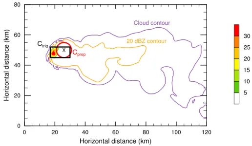
Christian et al., 1999;Ushio et al., 2003;Ott et al., 2007). This region is defined by the convective core and by the region extending 10 km downwind of the maximum vertical velocity (Ctrig) (Fig. 1). The downwind direction is assumed to be the mean wind direction at the altitude where both non-precipitation and precipitation ice particles

5

are encountered. The center of the region where an individual flash can propagate is chosen randomly among all the points of the cylinder that are in the glaciated part of the cloud. Another cylinder C_prop where a lightning flash can propagate (radius 4 km but could depend on the flash length) is centered on the randomly chosen point. The points of the cylinder where the discharge can propagate are restricted to the region of

10

the cloud where ice particles can be found since the hydrometeors that carry most of the electric charges are the ice particles (Barthe and Pinty,2007a).

The vertical distribution of the flash channel follows a bimodal distribution (DeCaria

et al.,2000,2005;Ott et al.,2007). This kind of structure is the most commonly ob-served (Shao and Krehbiel, 1996;Krehbiel et al., 2000; Rison et al., 1999; Thomas

15

et al.,2001;Wiens et al.,2005;Bruning et al.,2007) and simulated by explicit electrical schemes (Mansell et al.,2002;Barthe and Pinty,2007b). For each altitude level, the grid points reached by the lightning channel are chosen randomly among the possible points in the cylinder Cpropto mimic the filamentary and tortuous aspect of a lightning flash (Ott et al., 2007). The flash length of the lightning flash is prescribed either to

20

be constant or to have a lognormal distribution (Defer et al.,2003;Pinty and Barthe,

2008).

The amount of NO produced per flash is assumed to depend on the flash length and on the altitude (Wang et al.,1998):

n_{NO(P ) = a + bP} (2)

25

with n_NO the number of NO molecules produced per flash length (molecules m−1_), P the pressure (Pa). Wang et al. (1998) set the coefficients to a=0.34×1021 and b=1.30×1016. However, a wide range (1–13×1021molecules NO m−1 of flash)

ACPD

Full Screen / Esc

Printer-friendly Version Interactive Discussion has been determined from observations, laboratory experiments or modeling studies

(H ¨oller et al.,1999;Stith et al.,1999;Huntrieser et al.,2002;Skamarock et al.,2003;

Ott et al.,2007).

The aim of this new parameterization is to reproduce the global morphology of a lightning flash in terms of spatial distribution and length in order to avoid the

instan-5

taneous dilution of the NO in the storm. This is important for the redistribution of the chemical species and for the comparison between model results and observations.

3 Experimental and model design

The lightning-produced NOxparameterization described above has been placed in the Weather Research and Forecasting (WRF) model. Simulations of the 10 July 1996

10

STERAO storm have been conducted to evaluate and assess its sensitivities. 3.1 The WRF model

The WRF model solves the conservative (flux-form), non-hydrostatic compressible equations using a split-explicit time-integration method based on a 3rd order Runge-Kutta scheme (Skamarock et al.,2005;Wicker and Skamarock,2002). Scalar transport

15

is integrated with the Runge-Kutta scheme using 5th order (horizontal) and 3rd order (vertical) upwind-biased advection operators. Transported scalars include water vapor, the different hydrometeor categories and the chemical species. The cloud microphysics is described by the single moment (bulk water) approach (Lin et al.,1983). Mass mix-ing ratios of cloud water, rain, ice, snow, and graupel/hail are predicted. Cloud water

20

and ice are monodispersed and rain, snow, and hail have prescribed inverse expo-nential size distributions. For the graupel/hail category, the intercept parameter of the exponential distribution is 4×104m−4and the density is 917 kg m−3which corresponds to characteristics of hail particles.

The model predicts the mixing ratios of methane (CH4), carbon monoxide (CO),

ACPD

Full Screen / Esc

Printer-friendly Version Interactive Discussion ozone (O₃), hydroxyl radical (OH), hydroperoxy radical (HO₂), methyl hydroperoxy

rad-ical, nitrogen dioxide (NO2), nitric oxide (NO), nitric acid, hydrogen peroxide (H2O2), methyl hydrogen peroxide, formaldehyde (CH2O), formic acid, sulfur dioxide, ammo-nia, and aerosol sulfate (Barth et al., 2007a). The gas-phase chemistry represents O3-NOx-CH4 chemistry, but not non-methane hydrocarbon chemistry which likely has

5

a negligible effect on NOxmixing ratios in the anvil. Species are partitioned between the gas and aqueous phases via Henry’s law equilibrium for low solubility species (e.g. CO) or via diffusion-limited mass transfer for high solubility species (Barth et al.,2001). The aqueous chemistry occurring in the cloud water and rain represents OH and HO2 oxi-dation of dissolved species plus the oxioxi-dation of S(IV) by O₃and H₂O₂. The pH of the

10

drops is iteratively calculated via a charge balance assuming CO2 is 360 µmol mol−1. The chemical mechanism is solved with an Euler backward iterative approximation us-ing a Gauss-Seidel method with variable iterations. A convergence criterion of 0.01% is used for all the species. The dissolved species are transferred to other cloud hy-drometeors via microphysics processes (Barth et al.,2001). When cloud or rain drops

15

freeze, it is assumed that all of the dissolved species is retained in the frozen hydrom-eteor. In addition, adsorption of gas-phase nitric acid, sulfur dioxide, formaldehyde, and hydrogen peroxide is represented using the Langmuir equilibrium model approach (Tabazadeh et al.,1999;Popp et al.,2004).

In addition to the chemically active species, a tracer of NOx from lightning (LNOx)

20

is included in WRF. The LNOx tracer corresponds to the NO mixing ratio produced by lightning flashes. LNOx is transported only and does not undergo any chemical reactions.

3.2 The 10 July 1996 STERAO storm

The LNOx production in the 10 July 1996 STERAO storm has been widely studied

25

(Stith et al.,1999;Skamarock et al.,2003;Barthe et al.,2007b;Barth et al.,2007a,b). Different parameterizations and different models have been used to simulate this storm leading to a wide range of values for the production rate estimate. Large differences

ACPD

Full Screen / Esc

Printer-friendly Version Interactive Discussion are found in LNO_xestimates that range from 36 moles per flash to 465 moles per flash

(Barth et al.,2007b). Thus, it is interesting to investigate the origin of such discrepan-cies and to evaluate the uncertainties associated with each step of the LNOx param-eterization. The 10 July 1996 storm has also been chosen because there is a unique set of data for this storm: storm structure and kinematics from radar data, lightning

5

flash characteristics and in-situ chemical species measurements from two aircraft (Dye

et al.,2000).

During the STERAO-A experiment the ONERA VHF interferometeric mapper (ITF) measured the total (IC+CG) lightning activity while the National Lightning Detection Network (NLDN) documented the CG activity (Dye et al.,2000). NLDN provided

lo-10

cations of the ground connections from the measurements of the electric and mag-netic field due to the high current of return strokes (Cummins et al.,1998). ITF was designed to detect and locate VHF radiation emitted during both IC and CG flashes (Defer et al.,2001). VHF radiation is recorded during stepped leaders, dart leaders, recoil streamers and return strokes of negative CGs (Defer et al.,2001). Comparison

15

between optical radiation detected by NASA Optical Transcient Detector (OTD) and VHF radiaton recorded by ITF for one passage over the STERAO-A domain (9 July 1996) showed consistent observations between OTD and ITF (Defer et al.,2006), sug-gesting that a flash sensed by OTD corresponds to a flash sensed by ITF. However,

Boccippio et al.(2002) estimated the flash detection efficiencies to be 93% (nighttime)

20

and 73% (local noon) for LIS and 56% (nighttime) and 44% (local noon) for OTD. Thus, extrapolations of the results reported here must be done cautiously as the detection of flashes by satellite instruments is less than that by the ITF system. Further, the 10 July 1996 STERAO storm is likely not a typical thunderstorm whose flash, physical structure, and dynamics characteristics are necessarily meaningful for extrapolation of

25

ACPD

Full Screen / Esc

Printer-friendly Version Interactive Discussion

4 Control experiment

4.1 Initialization

The simulation performed is similar to those described by Skamarock et al. (2000,

2003) andBarth et al.(2001,2007a). The environment was assumed to be homoge-neous, thus a single profile was used for initialization. The initial profiles of the

mete-5

orological data were obtained from sonde and aircraft data (Skamarock et al.,2000). The convection was initiated with three warm (3◦C perturbation) bubbles oriented in a NW to SE line. WRF is configured to a 160×160×20 km3domain with 161 grid points in each horizontal direction (1 km resolution) and 51 grid points in the vertical direction with a variable resolution beginning at 50 m at the surface and stretching to 1200 m at

10

the top of the domain. The simulation was integrated at a 10 s time step. To keep the convection near the center of the model domain, the grid is moved at 1.5 m s−1 east-ward and 5.5 m s−1 southward. The simulation was integrated for a 3-h period. While the observed storm lasted from 21:30 to 03:00, only the multicell and supercell stages are simulated. These stages correspond to 23:15–02:15 UTC in the observations.

15

Initial mixing ratios of the chemical species are the same as those in Barth et al.

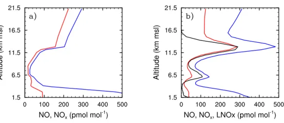
(2007a). Of interest to this study are NO, NO2 and O3 mixing ratios. NO and NOx initial mixing ratios are relatively high near the surface, low in the mid-troposphere, and moderately high in the UTLS region (Fig.2). O3 mixing ratios are 60 ppbv near the surface and are fairly constant with height to 12 km m.s.l. where mixing ratios increase

20

into the stratosphere. Because of the short integration time and small domain, there is very little effect of lightning-produced NO on O3mixing ratios in these simulations. The initiation process is the same in all the simulations.

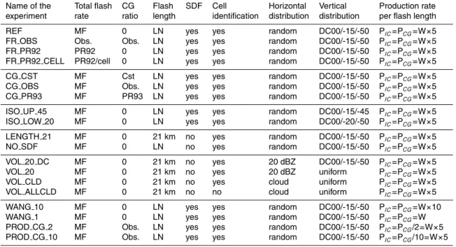
The details of the control experiment (REF) are summarized in Table1. The total flash rate is computed from the non-precipitation and precipitation ice mass flux

prod-25

uct. The cloud-to-ground flash rate is considered null all along the simulation since very few CG flashes were observed in this storm (83 CG flashes of both polarities and 5428 total flashes between 21:52 and 03:00 UTC). The lower and upper modes of the

ACPD

Full Screen / Esc

Printer-friendly Version Interactive Discussion bimodal distribution correspond to the −15◦_{C and the −50}◦_{C isotherms, respectively.}

The flash length of an individual storm is assumed to be lognormal in the range 1 to 400 km. As in the observations (Defer et al.,2001,2003), the percentage of the short flashes (<1 km) is set to 47%. Among these short flashes, 36% are considered as short duration flashes (<1 ms). In this simulation, it is assumed that the short duration

5

flashes produce as much NO molecules per flash length as a normal short flash. The production rate of NO per flash depends on the flash length and on the pressure. The original a and b parameters of Wang et al.(1998) have been multiplied by 5 to best match with observations (aREF=1.7×10

21 and bREF=6.5×10 16 ). 4.2 Results 10

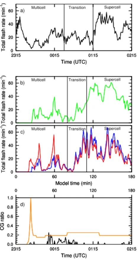
The dynamics and the microphysics structure of this storm has been studied previously (Skamarock et al., 2000, BDB07). These studies showed that the WRF simulations compare well to the radar data. Based on the storm structure and dynamics, three dif-ferent stages have been identified in this storm: a multicell (0–80 min corresponding to 23:15–00:30 UTC), a transition (80–110 min corresponding to 00:30–01:05 UTC) and a

15

supercell (110–180 min corresponding to 01:05–02:30 UTC). For comparison of obser-vations to the model results, the number of observed lightning flashes are reported for the period 23:40 to 02:15.

First, the flash rate computed from the ice mass fluxes is compared to observations. The simulated and observed total flash rates are shown in Fig.3a and b. The number

20

of flashes observed between 23:40 and 02:15 UTC was 3728, while that simulated was 4253 flashes for the 3-h simulation. The first simulated flash occurs after 25 min of simulation. In the multicell stage, several cells are at different evolution stages, so the extreme values and the average values of the flash rate are compared. The minimum and maximum values in the REF simulation are 2 and 39 fl. min−1, respectively, which

25

is similar to the minimum and maximum observed values (3 and 34 fl. min−1_{; Table3).} The mean flash rate during the multicell stage is 9.2 fl. min−1for the simulated flash rate, which is similar to the 10.5 fl. min−1observed. During the transition stage, the ice mass

ACPD

Full Screen / Esc

Printer-friendly Version Interactive Discussion flux parameterization underestimates the mean flash rate (15.7 vs. 20.4 fl. min−1) and

overestimates it in the supercellular stage (43.8 vs. 33.8 fl. min−1). BDB07 have shown that the supercellular stage begins earlier in the simulation compared to observations and the simulated mass flux is larger than observed in this stage of the storm. The differences in the simulated and observed microphysics and dynamics features cause

5

the differences in the observed and simulated flash rate.

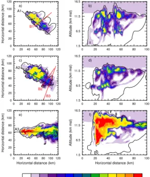
Figure4 shows horizontal and vertical cross sections of the NO mixing ratio during the different stages of the storm. During the multicell stage, NO production by lightning occurs mainly in the convective cores. At 3600 s, five different cells are present in the domain: three of them are located along a NW-SE axis as initialized and the two others

10

are on the eastern side of the NW and middle cells. Peaks of NO up to 3000 pmol mol−1 are colocated with the cells (Fig.4a). NO mixing ratios higher than 1000 pmol mol−1 are related to fresh production of NO by lightning flashes. Downwind of the convective cores (SE of the storm cores), NO values lower than 1000 pmol mol−1 are due to the transport and dilution of NO produced by lightning earlier in the simulation. Figure4b

15

shows that high values of the NO mixing ratio are mainly located in the range 6–7.5 km altitude and 11–14 km altitude due to the bimodal distribution of the flash segments.

At 5400 s, the flash rate is lower than in the multicell stage (see Fig. 3) which can explain why peak NO values decrease (Fig.4c). NO starts to spread over a large region in the anvil. The vertical cross section during the transition stage (Fig.4d) confirms that

20

less LNO_xis produced at this time of the simulation.

In the supercell stage (t=7200 s), the flash rate is higher than in the two other stages with values in the range 19–61 fl. min−1 leading to high values of the NO mixing ratio. In the anvil, values higher than 4000 pmol mol−1 _{extend horizontally for 25 km from} the convective core. NO mixing ratios up to 1000 pmol mol−1 can be found 100 km

25

downwind of the updraft maximum. Even though the LNOx parameterization produces LNO_xonly in a small region in and downwind of the convective core, NO molecules are transported and diluted in the whole cloud. Lightning flashes are then responsible for a large amount of NO in the whole system during the supercell stage (Fig.4f).

ACPD

Full Screen / Esc

Printer-friendly Version Interactive Discussion The NO mixing ratios from the model are next compared to the University of North

Dakota’s (UND) Citation aircraft measurements. The observed NO vertical cross-section (Fig. 5) is a result of projecting the NO aircraft measurements collected be-tween 23:16 and 00:36 UTC onto the across-anvil plane, which is ∼60 km downwind of the convective core. Several regions of NO mixing ratio higher than 540 pmol mol−1

5

can be seen at the altitude of 11.5 km and up to 13 km which is in agreement with observations (Fig.5).

NO transects across the anvil during the multicell and the transition stage of the storm have been plotted in Fig.6. After 1 h of simulation, the transect is 10 km down-wind of the southeastern cell. The simulated transect compares well with observations.

10

A peak of 1800 pmol mol−1 _{is simulated and NO>500 pmol mol}−1 _{extends over a} dis-tance of 20 km in the simulation. The disdis-tance over which the observed NO mixing ratio is higher than 500 pmol mol−1 is 30 km. Thus, WRF with its new LNOx parameteriza-tion is able to simulate peaks of NO higher than 1000 pmol mol−1 _{in the region where} lightning flashes are mostly triggered and propagate. After 1 h 30 min of simulation,

15

the transect is located 50 km downwind of the main convective core. The trends of the simulated and observed transects are the same, however the simulated values are lower in magnitude compared to the observations. The lightning activity in this storm started at 21:52 UTC, i.e. 108 min before the first flash was triggered in the simulation (25 min after the beginning of the simulation or 23:40 UTC). NO may have accumulated

20

in the environment of the storm leading to larger values than simulated. In summary, the WRF model coupled with the new LNOx scheme gives results in good agreement with observations both near the convective cores and in the anvil.

The effect of the transport and lightning production of NO can be seen by comparing NO and NOxfinal mixing ratios with their initial values. Figure2shows the NO, NOxand

25

LNO_x (a tracer of NO produced from lightning) vertical profiles horizontally-averaged over the model domain after 3 h of simulation. The NO and NOx vertical profiles are impacted by transport, chemistry processes and lightning flashes. The NOx in the boundary layer is efficiently transported in the mid- and upper troposphere by the

up-ACPD

Full Screen / Esc

Printer-friendly Version Interactive Discussion draft. The NOx mixing ratio at the ground is reduced from 600 pmol mol−1 (Fig.2a) to

350 pmol mol−1 (Fig. 2b). When comparing the NO and LNOx curves, it can be seen that the two peaks at 13.0 km m.s.l. and 6.5 km m.s.l. are caused by NO production by lightning flashes. The intense vertical motions and the high electrical activity in the 10 July 1996 STERAO storm causes the modeled NO mixing ratio to increase by 120% at

5

13 km m.s.l. and by 400% at 6.5 km m.s.l.

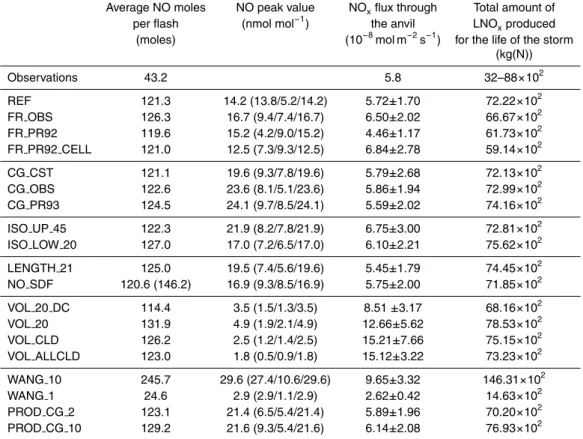
The simulated NOx flux through the anvil is 5.72×10−8moles m−2s−1, which is sim-ilar to the value derived from observations reported by Skamarock et al. (2003) of 5.8×10−8_{moles m}−2_s−1 _{(Table 2). In this simulation, a typical flash is 21.7 km long.} The mean production rate per flash calculated by dividing the total production of NO

10

by the total number of flashes is 121.3 moles of NO (7.3×1025 molecules NO). This production rate is in the lower range of the estimates from the last 5 years as reported bySchumann and Huntrieser(2007). Furthermore, our estimate is lower than most of the 3-D CRM studies.

5 Sensitivity analyses

15

To examine the key processes in the LNOx parameterization for CRMs, the sensitivity of the NO mixing ratio to several parameters is investigated. In particular, the impact of the total flash rate, the CG rate, the flash length, the short duration flashes, the spatial distribution of the NO molecules, and the NO production rate per flash are studied. A summary of the name and conditions of the experiments is given in Table1.

20

5.1 Total flash rate

When simulating the production of LNO_xin thunderstorms, the total flash rate is funda-mental. Two different parameterizations for the total flash rate have been tested in this section and compared to observations from the ONERA interferometer (Defer et al.,

2001). First, the total flash rate can be deduced from the non-precipitation and

ACPD

Full Screen / Esc

Printer-friendly Version Interactive Discussion cipitation ice mass flux product as described in Sect. 2 (Eq. 1) and used in the REF

simulation. Secondly, a sensitivity simulation is performed using the flash data from the ONERA interferometer (FR OBS, Table1). To determine the flash rate in each convec-tive cell i , the cell flash rate (F(i )) is assumed to be in proportion to the cell ice mass flux product (f(i )). That is,

5 F(i ) _{= F ×} f (i ) P (i )f(i ) (3)

where F is the total flash rate. Thirdly, the total flash rate can be determined from the maximum vertical velocity w_max(m s−1_{) followingPrice and Rind(1992):}

F_{P R = 5.7 × 10}−6

× wmax4.5 (4)

Two different simulations use thePrice and Rind (1992) approach for the flash rate.

10

In the first simulation, wmaxis the maximum vertical velocity in the whole domain: the total flash rate is then computed for the whole domain (FR PR92). The distribution of the flash rate in each cell is in proportion to the cell ice mass flux product (Eq.3). Because thePrice and Rind(1992) parameterization has been used several times in CRMs (Pickering et al., 1998; Fehr et al., 2004; Barth et al., 2007b) where several

15

cells can be identified, a second simulation in which the total flash rate per cell is computed from the maximum vertical velocity in each individual cell (FR PR92 CELL) is performed. That is, Eq. (4) is applied for each cell. Equation (4) has been rescaled for the FR PR92 and FR PR92 CELL simulations in order to best match with observations. For FR PR92 and FR PR92 CELL, Eq. (4) is multiplied by 0.19 and 0.16, respectively,

20

to have approximately the same total number of flashes as observed.

Results of the total flash rate in each simulation is compared to that predicted by the ice mass flux product and to the observed flash rate. In the REF and FR PR92 simulations, the first flash is triggered at 25 min while the lightning activity starts at 19 min in FR PR92 CELL, i.e. only 3 min after ice particles start to form in this simulated

25

ACPD

Full Screen / Esc

Printer-friendly Version Interactive Discussion collision between more or less rimed ice particles (Takahashi,1978;Jayaratne et al.,

1983;Saunders et al.,1991, e.g.). Using an explicit electrical scheme in a CRM,Barthe

and Pinty (2007b) showed that the first flash was triggered 20 min after ice particles appeared in the cloud. Since the maximum vertical velocity in their simulated storm did not exceed 20 m s−1_{, a shorter delay can be expected in the 10 July storm which is}

5

more intense. The simulated 10 July STERAO storm starts to produce ice particles at 16 min and the flux hypothesis allows the first flash to be triggered at 25 min, i.e. 9 min later. In the FR OBS simulation, the observed flash rate is available since 21:52 UTC, but it is only taken into account starting at 25 min (23:40 UTC) to allow the cloud to develop, to electrify and to trigger lightning.

10

As some differences exist between the time of the observed and simulated stages of this storm, the lightning activity is compared in each stage. Table3 shows highly variable results for FR PR92 and FR PR92 CELL. An important point is that the flash rate in FR PR92 and FR PR92 CELL is in advance compared to REF and to observa-tions (Fig.3). For example, at the end of the transition stage the total flash rates in the

15

FR PR92 and FR PR92 CELL simulations increase 10 min before the REF simulation and the observed flash rate increase. In thePrice and Rind(1992) parameterization for the total flash rate, only the maximum vertical velocity is considered. There is no information about the ice content or about conditions favorable for the non-inductive separation mechanism which can lead to this lag. Thus, contrary to the total flash rate

20

deduced from the flux hypothesis, the total flash rate fromPrice and Rind(1992) seems to be not as suitable for use in CRM as it does not take into account the microphysical development of the storm which is of primary importance for the cloud electrification. Using an explicit electrical scheme to simulate a STEPS supercellular storm,Kuhlman

et al. (2005) concluded that there is no correlation between the maximum vertical

ve-25

locity and the total flash rate. Deierling (2006) confirmed this conclusion using radar and lightning data.

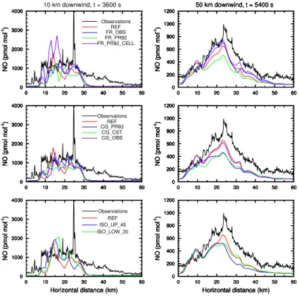
To examine the effect of using different flash rate parameterizations, the NO mixing ratio downwind of the convective core is analyzed. Figure5 shows the vertical cross

ACPD

Full Screen / Esc

Printer-friendly Version Interactive Discussion sections of the NO mixing ratio across the anvil at 6000 s. The REF, FR OBS and

FR PR92 CELL simulations display similar results having several spots in the anvil with NO mixing ratio >500 pmol mol−1. The lower values of the NO mixing ratio in the anvil for the FR PR92 simulation are not due to the lower flash rate during the transition stage (Fig.3) since 1193 flashes are produced in FR PR92 and 1184 in REF,

5

but instead are attributed to the lower flash rate during the multicell stage (487 flashes in FR PR92 and 728 flashes in REF). Indeed, NO molecules are produced mostly near the convective core and it takes ∼40 min to be transported in the anvil to 50 km downwind. Because the number of flashes in the multicell stage is higher for FR OBS and FR PR92 CELL than for the REF simulation, the NO mixing ratios for FR OBS

10

and FR PR92 CELL are also higher than those for REF in the vertical cross section at 6000 s. Along the transects across the convective core during the multicell stage (Fig.6), all the simulations exhibit peaks higher than 1000 pmol mol−1 characteristic of local production of LNO_x. The peak of NO reaches 2700 pmol mol−1_{in FR PR92 CELL,} which is the simulation with the most flashes in the first hour, and 1200 pmol mol−1 in

15

FR PR92, the simulation with the fewest flashes before 1 h. The simulations producing more LNO_xnear the convective core (transect 10 km downwind at 3600 s) are the ones that have more NO transported in the anvil (transect 50 km downwind at 5400 s).

The NOx flux through the anvil varies from 4.46×10−8mol m−2s−1 for FR PR92 to 6.84×10−8mol m−2s−1 for FR PR92 CELL. As with the NO mixing ratios 50 km

down-20

wind of the convective cells, the NO_x flux depends on the lightning flash rate during the multicell stage of the storm because of the >40 min of transport time from the con-vective cells to the location of the flux calculation. An increase of 79% in the flash rate is related to an increase of 53% in the NO_x flux through the anvil. The non-linear change between changes in flash rate and NOxflux from these two simulations is due

25

to the placement of the flashes and therefore the placement of the NO source. The FR PR92 CELL simulation distributes the NO source according to w_maxin the individ-ual cells, while the FR PR92 simulation distributes the NO source according to the ice mass flux product (Eq.3). These locations may be similar but not necessarily exactly

ACPD

Full Screen / Esc

Printer-friendly Version Interactive Discussion the same.

5.2 Cloud-to-ground flash rate

Boccippio et al. (2001) analyzed four years of OTD and NLDN flash rate data over the United States and found that the CG to IC ratio may be dominated by storm type, morphology and level of organization instead of environmental parameters. Here, we

5

examine the influence of the CG to IC ratio on the NO mixing ratios. In this study, the cloud-to-ground ratio α is defined by:

α = NCG

N_{IC+ NCG} (5)

Price and Rind(1993) estimated the cloud-to-ground ratio α_{P R} from the depth Z of the layer from the freezing layer to the cloud top (simulation CG PR93).

10 α_{P R =} 1 1 + β (6) with: β = NIC N_CG = 0.021Z4− 0.648Z3+ 7.493Z2− 36.54Z + 63.09 (7)

N_ICand N_CG are the number of IC and CG flashes, respectively. The cloud top height

15

is computed taking the average altitude where the total hydrometeor mixing ratio de-creases to 10−5kg kg−1. Two other simulations (Table1) have been performed with the observed α_OBS ratio (CG OBS), and with a constant value (CG CST). The constant value is αCST=0.02 which corresponds to αOBS averaged during the simulated storm. These simulations are compared to REF in which CG flashes are not considered.

20

Figure 3 displays the observed and simulated N_CG/(N_IC+NCG) ratio. The αP R ratio

ACPD

Full Screen / Esc

Printer-friendly Version Interactive Discussion equals 4850 m. Then, as the storm is developing and extending vertically, the αP R ratio

decreases rapidly to values ∼0.2. This value is 10 times larger than the mean α (0.018) deduced from observations between 23:15 and 02:15 UTC. Even when the observed convection started, αOBSdid not reach such high values.Lang et al.(2000) studied this anomalously low CG rate in two STERAO storms and concluded that it could originate

5

from an elevated charge region (MacGorman et al.,1989). MacGorman et al.(1989) hypothesized that strong updrafts can suspend the negative charge center to higher altitudes than in ordinary storms. This elevated charge would favor IC flashes over CG flashes. Here, we can investigate the impact of the high α ratio on the LNOxproduction compared to the other simulations.

10

Pickering et al.(1998) used Eq. (7) to estimate the CG ratio in seven different storms. In the two mid-latitude continental events in which CG flash data were available, the simulated CG rate was in reasonable agreement with observations. For the total flash rate in the simulated 21 July 1998 EULINOX storm,Fehr et al.(2004) rescaled Eq. (7) by a factor of 1.10. As for the total flash rate estimated by thePrice and Rind (1992)

15

parameterization, it is not clear if Eq. (7) needs to be rescaled depending on the storm or on the model. More tests should be done on several convective cases with the same model and with available observations.

When comparing the NO mixing ratios along the transects and in the vertical cross section across the anvil (Figs.5 and 6), the CG OBS results are in better agreement

20

with the REF simulation and with observations than CG PR93 and CG CST results. The CG PR93 and CG CST results have NO mixing ratios lower than the observations both in the convective region and in the anvil. Consequently, it is important to have the right number and temporal distribution for the CG flashes. Because the α_{P R}ratio is ∼10 times greater than αOBS, more NO is produced in the mid troposphere at the expense of

25

the upper troposphere resulting in a 33% increase of NO in the mid-troposphere and a 20% decrease in the upper troposphere (Fig.8). However, even if the NO mixing ratio is low compared to the reference run and to the observations, it reaches 1000 pmol mol−1 in the transects 10 km downwind.

ACPD

Full Screen / Esc

Printer-friendly Version Interactive Discussion Despite an increase in the CG rate by a factor 10 between CG CST and CG PR93

(the total number of flashes being constant), NO produced by lightning is not signif-icantly impacted. It causes a decrease of 3.5% in the flux through the anvil and an increase of 2.8% in the total amount of nitrogen produced during the storm lifetime. The flux through the anvil is decreased when there are more CG flashes because even

5

if more NO molecules are produced, they are produced at lower altitudes and it takes more time to be transported in the anvil.

5.3 Altitude of the upper and lower modes for the bimodal distribution

Typically the IC discharge has a bilevel structure (Shao and Krehbiel,1996), which is correlated with the main negative and upper positive charge regions of the storm.Rison

10

et al. (1999),Thomas et al.(2001) andKrehbiel et al.(2000) deduced from the use of the Lightning Mapping Array in New Mexico and Oklahoma that the main negative charge is located in the middle level at 5–6 km m.s.l. while the upper positive charge is centered at about 10–12 km altitude. By examining electric field soundings in different thunderstorms,Stolzenburg et al.(1998) found that the temperature at the center of the

15

main negative charge region varies from −4◦C to −32◦C with a mean value of −15.7◦C. Thus, the production of NO_xand its subsequent distribution by updrafts and downdrafts may be sensitive to the altitudes chosen for the bimodal distribution.

Two sensitivity tests have been performed to investigate the impact of a change in the altitude of the two levels where flash segments are preferentially distributed on the

20

LNO_x mixing ratio and budget. First, the upper isotherm is set to −45◦_{C (simulation} ISO UP 45) instead of −50◦C in the REF simulation. Second, the lower isotherm is set to −20◦C (ISO LOW 20) instead of −15◦C in REF to account for the hypothesized elevated charge mechanism in this storm (Lang et al.,2000).

Using the −45◦C isotherm as the upper level for the flash segments

distribu-25

tion mainly shifts the LNOx production in the upper troposphere to the altitude of 11.5 km m.s.l. instead of the 12 km m.s.l. In the convective core and slightly downwind, the NO mixing ratio is fairly similar in the REF, ISO UP 45 and ISO LOW 20

simula-ACPD

Full Screen / Esc

Printer-friendly Version Interactive Discussion tions (Fig. 6). However, it is slightly higher in ISO UP 45 and ISO LOW 20 than in

REF. The LNOx produced in the lower mode for ISO LOW 20 is more readily available at high altitude than in the REF simulation.

The impact of moving the altitude of the upper and lower modes in the vertical dis-tribution of the flash segments has an impact on the flux of NOx through the anvil

5

(Table 2). Lowering the upper mode and raising the lower mode both result in an increase of the NO_x flux through the anvil. DeCaria et al.(2000) tested different tem-peratures (−40◦C and −30◦C) for the upper isotherm of their bimodal distribution in the 12 July 1996 STERAO storm. They found that by lowering the upper mode of the flash distribution the maximum of the NO plume occurs at a lower altitude.

10

5.4 Flash length

Previous studies have estimated the flash length to be in the range 20–50 km (Th ´ery

et al.,2000). For the 10 July 1996 STERAO storm analysis, Defer et al. (2001) have shown that the flash length in this storm is not constant and varies from 0.02 and 474 km. They have concluded that the average value of the flash length is 19 km but

15

is 34 km if short duration flashes (flashes <1 ms) are not considered.Pinty and Barthe

(2008) conducted an ensemble of simulations of two idealized electrified storms with a cloud-resolving model coupled to an explicit electrical scheme. They showed that the number of segments in an individual flash is highly variable from flash to flash but looks like a lognormal distribution.

20

To explore the importance of the flash length to the production of NO from lightning, a simulation is performed using a constant flash length of 21 km (LENGTH 21, Table1). The value of 21 km corresponds to the mean flash length simulated when a lognor-mal distribution for the flash length is used and when short duration flashes are taken into account. The aim of these sensitivity tests is to investigate the impact of using a

25

constant or a varying flash length.

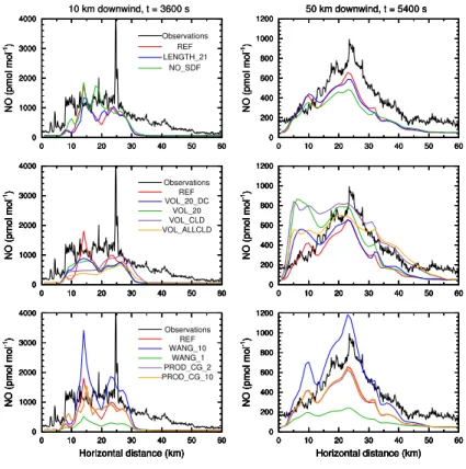
Using the more realistic lognormal distribution for the flash length (REF) leads to re-sults fairly similar to a constant value (LENGTH 21) in the convective core and

down-ACPD

Full Screen / Esc

Printer-friendly Version Interactive Discussion wind. The main difference arises in Fig.8where the LENGTH 21 and REF profiles

dif-fer between 5.5 and 10.5 km m.s.l. These mean profiles show that LENGTH 21 tends to produce more NO molecules in the lower part of the cloud. This difference can be due to the treatment of the short flashes <1 km since they are made up of only one point. Due to the bimodal vertical distribution that is used, the short flashes tend to be

5

produced in the upper part of the cloud (∼12 km m.s.l.). This is slightly higher than the analysis ofDefer et al.(2001) who showed that the VHF sources with strong radiation were mostly located in altitude between 7.5 and 10.5 km m.s.l. The increase of sources at lower altitude increases the NO production per flash from 121.3 moles fl.−1in REF to 125.0 moles fl.−1 in LENGTH 21 (=3.1%) because of the pressure dependence in the

10

NO production (Eq.2). 5.5 Short duration flashes

In the 10 July 1996 STERAO storm, Defer et al. (2001) defined the short duration flashes as discharges lasting less than 1 ms while the mean flash duration is 240 ms in this storm. They reported that between 22:50 and 23:30 UTC up to 45% of the

15

recorded flashes were short duration flashes.

Analyzing data from the lightning mapping array,Harlin et al.(2003) identified three different types of short duration flashes lasting less than 80 ms: the isolated events, the precursor events, and the high source power events. Several studies have shown that taking into account or not the short duration flashes does not modify the flash rate

20

trend but can significantly change its magnitude (Lang et al.,2000;Wiens et al.,2005). Whether these short duration flashes should be considered or not as part of the total lightning flash rate and as a source of nitrogen oxides is a matter of debate.

To investigate the possible impact of short duration flashes in the LNO_xproduction, a sensitivity simulation (NO SDF) has been performed. In this simulation, the lognormal

25

distribution is used but it is hypothesized that the short duration flashes do not produce NO molecules. It is worth recalling that the reference run (REF) assumes that short duration flashes produce as many NO molecules per meter of flash as “normal” flashes.

ACPD

Full Screen / Esc

Printer-friendly Version Interactive Discussion It is assumed that the flash length of a short duration flash is 1 km, and that 36% of the

flashes that are 1 km in length are short duration flashes.

In the NO SDF simulation 4253 flashes have been triggered among which 699 were short duration flashes. If short duration flashes are not considered in the total flash rate, 146.2 moles of NO are produced per flash on average. If the total amount of NO

5

produced by lightning is divided by the total flash rate (4253), one flash produces on average 120.6 moles of NO.

If short duration flashes are assumed to produce as many molecules per meter of flash as a normal flash, their impact on the NO mixing ratio is not significant. In Figs.5,

7and8, the NO SDF and REF simulations give similar results. As noted in the previous

10

section, the simulated short flashes are mostly produced at altitudes between 11 and 12 km m.s.l., which is higher than in the observations.

Even though this sensitivity test concludes that short duration flashes are not very important for the LNO_x production, it must be kept in mind that little is known about the physics of these discharges. Thus the impact of the short duration flashes on the NO

15

budget should be studied further when more measurements of short duration flashes are available in conjunction with chemistry data.

5.6 Spatial distribution of the NO molecules

Previous parameterizations (Pickering et al., 1998; DeCaria et al., 2000, 2005) as-sumed that the NO molecules produced by the lightning flashes are instantly diluted

20

over the whole volume of the cloud or in the 20 dBZ contour. This instant dilution does not produce the NO peaks observed by instruments onboard airplanes (Barth et al.,

2007b;Ott et al.,2007). The goal of these sensitivity tests is to investigate how the NO mixing ratio is affected by an instantaneous dilution of the LNOxsource.

Four sensitivity tests are compared to the REF simulation. As in the REF simulation,

25

only IC flashes are considered. First, the approach ofDeCaria et al.(2005) is followed (VOL 20 DC, Table1). The NO molecules are distributed vertically following two modes in the volume where the radar reflectivity exceeds 20 dBZ. Second, the NO molecules

ACPD

Full Screen / Esc

Printer-friendly Version Interactive Discussion are distributed uniformly in the 20 dBZ volume above the −15◦_{C isotherm (VOL 20).}

Third, the simulation VOL CLD followsPickering et al. (1998) where the LNOx is dis-tributed over the entire cloud above the −15◦C isotherm. In these first three simulations the LNO_x source is only distributed in the detected electrified cell in proportion to the flash rate of each cell. Finally, the last simulation (VOL ALLCLD) followsPickering et al.

5

(1998) like VOL CLD but there is no cell identification. In these four simulations, the flash length is held constant (21 km) since the sensitivity test in Sect.5.4has shown no significant impact of the flash length distribution. In the VOL 20 DC, VOL 20, VOL CLD and VOL ALLCLD, the NO molecules produced by a single flash are distributed over 9400, 4300, 17 700 and 23 400 grid points on average, respectively. In contrast, the

10

REF simulation places NO by a single flash on ∼20 grid points.

To identify the impact of the bimodal distribution on the NO mixing ratio, the re-sults of the VOL 20 DC and VOL 20 simulations are compared. In Fig.5, the cross section of NO mixing ratio across the anvil for VOL 20 DC is fairly similar to REF. The region of high NO mixing ratio is much larger in VOL 20 than in VOL 20 DC. The

15

study of VOL CLD and VOL ALLCLD results gives some insight on the impact of the cell identification. Figure5 shows that three different spots of NO mixing ratio higher than 540 pmol mol−1 are visible for VOL CLD. In VOL ALLCLD there is only one large region where the NO mixing ratio exceeds 540 pmol mol−1_{. When the vertical} distri-bution of the NO molecules is uniform (VOL 20, VOL CLD, VOL ALLCLD), the region

20

with high NO mixing ratio across the anvil (Fig.5) increases with the volume in which NO molecules are instantly diluted. Moreover this volumetric distribution of the NO molecules over a large area does not allow the peaks in the transects to be reproduced near the convective core where an enhancement in the NO mixing ratio is observed (Fig.7). In these transects (Fig.7), the NO mixing ratios near the convective core for

25

VOL 20, VOL 20 DC, VOL CLD and VOL ALLCLD are lower than observations, but are similar in magnitude to the observations 50 km downwind of the convective core.

The NO_x flux in all these simulations is larger than that determined from the obser-vations and in the REF simulation (Table2) because the NO lightning sources for the

ACPD

Full Screen / Esc

Printer-friendly Version Interactive Discussion VOL 20 DC, VOL 20, VOL CLD, VOL ALLCLD simulations are placed at thousands of

grid points, many of which are near and within the anvil (see 20 dBZ contour in Fig. 1). The VOL 20 DC NOx flux is similar to that predicted by other models simulating this storm (Barth et al.,2007b) indicating that their overprediction of the NO_x flux may be due to the larger region of the NO lightning source compared to the filamentary

re-5

gion in the REF simulation. Despite the significant differences in the NOx flux, the total amount of NO produced from lightning is fairly similar among these 4 sensitivity simulations and the REF simulation.

5.7 Production of NO per flash

A recent review of lightning production of NO reported that the LNOxproduction rate per

10

flash length varies from 1×1021to 13×1021molecules m−1(Schumann and Huntrieser,

2007). This large range of values has been obtained in different storms by different ways: laboratory experiments, modeling studies with different models and different parameterizations or airborne measurements. Barth et al.(2007b) have also reported a large range of NO moles produced per flash (between 36 and 465 moles of NO per

15

IC flash) for the same storm simulated here but using different models and different parameterizations.

The impact of the number of NO molecules produced per flash length unit is inves-tigated in this section. All the simulations use theWang et al. (1998) equation giving the number of molecules produced per meter of flash (Eq.2). The WANG 1 simulation

20

uses the original a and b parameters (see Sect.2), whereas the REF and WANG 10 simulations use 5 and 10 times the parameters, respectively.

This sensitivity analysis is the one that impacts most the NO mixing ratio both in the convective core and in the anvil. Figure5shows that the NO mixing ratio in the anvil in the WANG 10 simulation is far too high compared to observations. In WANG 10,

25

there is a large region with NO mixing ratio higher than 540 pmol mol−1 that extends over 50 km horizontally. Conversely, the WANG 1 simulation exhibits NO mixing ratio in the anvil less than 300 pmol mol−1_.

ACPD

Full Screen / Esc

Printer-friendly Version Interactive Discussion The large difference in the NO mixing ratio between the WANG 1, REF and

WANG 10 simulations can be also seen in Fig. 7. The NO moles per flash, the NO peak value, and the total amount of LNOx produced during the storm increase quasi-linearly as the a and b parameters increase (Table2). The NO mixing ratio increase is not exactly linear since it is impacted by the NOx chemistry. The values of the LNOx

5

average profiles are affected by changing the a and b parameters, but the trends are the same for the three simulations.

Two additional simulations are performed to study the impact of a larger NO produc-tion rate by CG flashes. Pickering et al. (1998) used the values given byPrice et al.

(1997) (111 mol(NO) IC−1 and 1113 mol(NO) CG−1) to simulate seven case studies

10

representing different environments. Following the method of Price et al. (1997) to determine the amount of NO produced per flash in the 21 July EULINOX storm,Fehr

et al. (2004) used the value of 350 mol(NO) CG−1. The 480 moles of NO produced per IC were obtained by a fit to observations. DeCaria et al.(2005) who simulated the 12 July 1996 STERAO storm using the GCE model with thePrice et al. (1997) method

15

determined that the IC mean production rate is 460 moles of NO per IC flash. They also concluded from their sensitivity tests that IC and CG flashes produce the same amount of NO per flash. However, they assumed an instantaneous dilution of the NO molecules and only compared with the column NOxmass from observations. Ott et al. (2007) deduced from their study that 360 moles of NO per flash matches best with

ob-20

servations. Thus, the value of 121 moles of NO produced per flash derived here for the 10 July 1996 STERAO storm is in the lower range of values used or deduced from previous CRM studies except when an explicit electrical scheme is used. In previous parameterizations, the number of NO moles per flash was mostly deduced fromPrice

et al. (1997) who suggested a ratio of 10 between the production rate per CG and IC,

25

or it was deduced from observations, but only in one part of the storm. Few of the previous studies have used a geometric approach for the flash segments distribution or compared the NO mixing ratio to observations in different regions of the storm.