HAL Id: hal-01108891
https://hal.archives-ouvertes.fr/hal-01108891
Submitted on 23 Jan 2015
HAL is a multi-disciplinary open access
archive for the deposit and dissemination of
sci-entific research documents, whether they are
pub-lished or not. The documents may come from
teaching and research institutions in France or
abroad, or from public or private research centers.
L’archive ouverte pluridisciplinaire HAL, est
destinée au dépôt et à la diffusion de documents
scientifiques de niveau recherche, publiés ou non,
émanant des établissements d’enseignement et de
recherche français ou étrangers, des laboratoires
publics ou privés.
Estimating length scales for tropospheric turbulence
from MU radar and balloon data
Hubert Luce, Richard Wilson, Francis Dalaudier, Fanny Truchi, Hiroyuki
Hashiguchi, Masayuki K. Yamamoto, Mamoru Yamamoto, Kantha Lakshmi
To cite this version:
Hubert Luce, Richard Wilson, Francis Dalaudier, Fanny Truchi, Hiroyuki Hashiguchi, et al..
Esti-mating length scales for tropospheric turbulence from MU radar and balloon data. 14th International
Workshop on Technical and Scientific Aspects of MST14/IMST1, May 2014, Sao José dos Campos,
Brazil. �hal-01108891�
Estimating length scales for tropospheric turbulence from MU rad
Estimating length scales for tropospheric turbulence from MU rad
ar and balloon data
ar and balloon data
Hubert Luce,Hubert Luce, Université
Universitéde Toulon, La de Toulon, La GardeGarde, France, France
Richard Wilson, F. Dalaudier, F. Richard Wilson, F. Dalaudier, F. TruchiTruchi LATMOS
LATMOS--IPSL, UPMC IPSL, UPMC UnivUnivParis 06, Univ. Versailles StParis 06, Univ. Versailles St--Quentin, CNRS/INSU, UMR 8190, Paris, FranceQuentin, CNRS/INSU, UMR 8190, Paris, France Hiroyuki Hashiguchi, Masayuki K. Yamamoto, Mamoru Yamamoto
Research Institute for Sustainable Humanosphere, Kyoto Universit
Research Institute for Sustainable Humanosphere, Kyoto University, y, UjiUji, Japan., Japan.
Lakshmi LakshmiKanthaKantha
Aerospace Engineering Sciences, University of Colorado, Boulder,
Aerospace Engineering Sciences, University of Colorado, Boulder,USAUSA This work is dedicated to the memory of Prof. Shoichiro Fukao,
Thorpe analysis Introduction
Instrumental set-up
The Middle and Upper Atmosphere radar (MUR) was operated in range imaging (FII) mode (5 frequencies) from 01 November 2013 16:00 LT to 09 November 2013 08:00 LT at a time resolution of 6.14 s (e.g. Luce et al. 2006). The radar beam was steered into 3 directions (vertical, and 10°off
zenith toward North and East). The range sampling was performed from 1.32 km to 20.37 km. The FII mode was used for imaging the turbulent and stable layers. The Doppler spectra and moments were estimated at the range resolution of 150 m.
MUR observations
Figures 1(a)-1(b): Height-time cross-section of vertical MUR echo power in range imaging mode for all the campaign. The passage of frontal zones are clearly visible. The smoothed appearance of the radar echoes in clouds and precipitations strongly differ with the appearance of the thin stratified layers in dry air. The detailed analysis of the synoptic conditions will be performed in a subsequent work.
Conclusions
ε
Estimating atmospheric turbulence parameters from ST radar measurements is an important issue. The methods used in the literature are based on the hypothesis that radar echoes at oblique incidence result from isotropic turbulence within the inertial subrange (e.g. Naström and Eaton, 2005). In such a case, the width of Doppler spectrum can be related to the turbulent energy dissipation rate . When the outer scale of turbulence is smaller than the dimensions of the radar volume, depends on the background stability N2(e.g., Hocking, EPS, 1999). The latter parameter is usually estimated from standard balloon measurements.
Our studies aim at estimating turbulence parameters by taking advantage of the high time resolution of radiosondes (1 sec) and concurrent radar observations. Wilson et al. (JAOT, 2011) showed that detecting turbulence from PTU measurements is possible by using Thorpe analysis (Thorpe, DSR, 1977) despite the instrumental measurement noise. The method was applied by Clayson and Kantha (JAOT, 2008) but without considering the noise effects. Turbulent layers can be directly identified through the detection of overturns produced by mixing and billows in dry or moist potential temperature profiles. The instrumental noise can lead to the detection of spurious layers especially in weakly stratified regions. Wilson et al. (JAOT, 2010) proposed objective selection criteria and procedures for minimizing noise effects. Wilson et al. (AMT, 2013) considered the air saturation effects.
The Thorpe analysis also provides an important length-scale, the so-called Thorpe length LTdefined as the root mean square of the Thorpe
displacements in a turbulent layer. This parameter is very frequently used for characterizing turbulence in oceans: most studies revealed equivalence between LTand outer scales of turbulence (Ozmidov or buoyancy scales), for fully developed turbulence with an inertial domain (e.g.
Smyth and Moum, JPO, 2000).
From an intensive MU radar-balloon campaign at Shigaraki MU observatory performed in 2011, Luce et al. (RS, 2014) showed that the deepest turbulent layers identified in the potential temperature profiles (typically 50-1000 m in depth) are generally associated with nearly isotropic radar echoes, consistent with the detection of turbulence by the radar. This result gives credence to the fact that it is relevant to combine radar and balloon observations for estimating turbulence parameters, at least in a statistical sense. Wilson et al. (JASTP, 2014) estimated energetic parameters (turbulent kinetic and potential energy, energy dissipation rates, eddy diffusion coefficients and heat fluxes) for a few cases of turbulent layers detected by both instruments. They also provided the first comparisons between the buoyancy and Thorpe scales for atmospheric turbulent layers. The energetic parameters and buoyancy scale can be estimated from the Doppler spectral width after carefully removing the non-turbulent contributions (e.g. Hocking, EPS, 1999).
In the present work, we show some new results obtained from a multi-instrumental observation campaign carried out on 01-09 November 2013 at Shigaraki MU observatory and from previous campaigns. The mathematical derivation and calculation procedures can be found in Wilson et al. (JASTP, 2014, http://dx.doi.org/10.1016/j.jastp.2014.01.005i) only the most important information is recalled here.
Meisei RS-06 GPS radiosonde
Vaisala RS92G radiosonde MU radar
Among the other instruments operated at the same time, two types of radiosondes (Vaisala RS92G and Meisei RS-06 GPS) were used. The specification of the Meisei radiosondes are given at http://www.meisei.co.jp/english/products/meteo/rs06g_gps_radiosonde.html. Both radiosondes provide PTU (and wind) profiles at a vertical sampling of 1 sec. A total of 36 radiosondes were launched during night periods every ~01 hour 30 min (except on 01-02 Nov during which Meisei and Vaisala radiosondes were launched simultaneously three times). Launching times are indicated by the red dots in Figures 1a and b. The PTU profiles collected from both radiosondes were processed for applying the Thorpe analysis
1b 1a cloud Frontal surface (see Figure 3) rain storm dry air dry air cloud cloud dry air dry air
Figure 2: Close up of Figure (1a) between 01-NOV 20:00 LT and 02-NOV 05:20 LT . The nearly straight lines show the balloon altitude vs time (red: Vaisala, Black: Meisei). V02/M03, V04/M05 and V06/M07 were launched almost simultaneously but separately. The profiles are the moist potential temperature profiles used for Thorpe sorting. They were estimated from the numerical integration of dry N2when relative humidity was below the saturation thresholds defined by Zhang et al. (2010) for Vaisala sondes (and also used for Meisei sondes here) or moist N (Lalas and Einaudi, JAS, 1974) when above. Also shown are the vertical profiles of at a vertical resolution of 50 m. (The vertical dashed line correspond to
N*2=0). The Meisei and Vaisala profiles are very similar. The N*2maxima generally coincide with radar echo enhancements.
θ∗¿ ¿ dz d g N*2= /θ*θ*/ M01 M03 V02 V04 M05 V05 M06 01 *
θ
03 / 02 ∗ θ 05 / 04 ∗ θ 07 / 06 ∗ θ 2 −1 e−4 1 e−3 *2 NFigure 3: Close up of Figure (1a) between 02-NOV 20:00 LT and 03-NOV 05:05 LT. The black curves show the moist N*2and the vertical dashed lines show N*2=0. Deep regions of weak stability can be seen in the height range 6.0-11.5 km and coincide with a smooth appearance of the radar echoes. These echoes are not aspect sensitive (see Figure 5). Their structure contrasts with the thin layering below 6.0 km and above 11.5 km where profiles of N*2show a succession of narrow peaks. A frontal surface (strong temperature and humidity increases) and the cloud base are indicated by the dotted blue line (and coincide with the strong peak of N*2. Deep (up to ~1 km) turbulent layers can be seen on both sides of the cloud base and within the clouds. The nearly vertical striations of the echoes underneath cloud can be the signature of KH billows or convective rolls as already reported from MUR observations in FII mode for such atmospheric conditions (e.g. Luce et al, MWR, 2010).
θ∗¿ ¿ θ∗¿ ¿ θ∗¿ ¿ θ∗¿ ¿ θ∗¿ ¿ θ∗¿ ¿ V10 M09 M11 V12 M13 V14 N∗ 2¿ ¿
Thorpe length LT – buoyancy scale LBcomparisons
Turbulence parameters
3
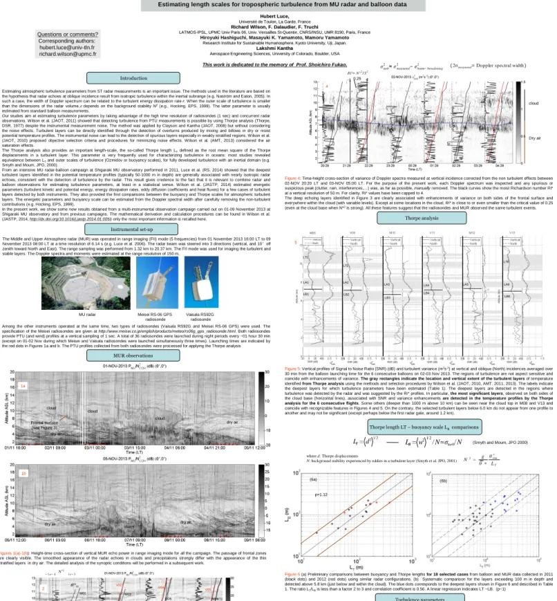
Figure 4: Time-height cross-section of variance of Doppler spectra measured at vertical incidence corrected from the non turbulent effects between 02-NOV 20:20 LT and 03-NOV 05:00 LT. For the purpose of the present work, each Doppler spectrum was inspected and any spurious or suspicious peak (clutter, rain, interferences,…) was, as far as possible, manually removed. The black curves show the moist Richardson number Ri* at a vertical resolution of 50 m. For clarity, Ri* values have been capped to 4.
The deep echoing layers identified in Figure 3 are clearly associated with enhancements of variance on both sides of the frontal surface and everywhere within the cloud (with variable levels). Except at some locations in the cloud, Ri* is close to or even smaller than the critical value of 0.25 (even at the cloud base when N*2is strong). All these features suggest that the radiosondes and MUR observed the same turbulent events.
cloud Dry air
σ
turb2≈ σ
measured 2−
σ
beam−broadening 2 4 Ri¿=N¿2/S2 -10.25 4 cloud Dry air(2σmeasured=Doppler spectral width)
Figure 5: Vertical profiles of Signal to Noise Ratio (SNR) (dB) and turbulent variance (m2s-2) at vertical and oblique (North) incidences averaged over 30 min from the balloon launching time for the 6 consecutive balloons on 02-03 Nov 2013. The regions of turbulence are not aspect sensitive and coincide with enhancements of variance. The gray rectangles indicate the location and vertical extent of the turbulent layers of temperature identified from Thorpe analysis using the methods and selection procedures by Wilson et al. (JAOT, 2010, AMT, 2011, 2013). The labels indicate the deepest layers for which turbulence parameters have been estimated (Table 1). The deepest layers are detected in the regions where turbulence was detected by the radar and was suggested by the Ri* profiles. In particular, the most significant layers, observed on both sides of the cloud base (horizontal lines), associated with SNR and variance enhancements are detected in the temperature profiles by the Thorpe
analysis for the 6 consecutive flights. Some others (deeper than 1000 m above 10 km) can be seen near the cloud top in M08 and V13 and
coincide with recognizable features in Figures 4 and 5. On the contrary, the selected turbulent layers below 6.0 km do not appear from one profile to another and may not be significant (except perhaps below the first radar gate, around 1.2 km).
5 2 / 1 2
d
=
L
T where d: Thorpe displacementsN: background stability experienced by eddies in a turbulent layer (Smyth et al. JPO, 2001)
N
σ
N
w
=
L
B/
turb/
2 / 1 2≈
T rmsL
θ
θ
g
=
N
*' 2∗
(6a) (6b)Figure 6(a) Preliminary comparisons between buoyancy and Thorpe lengths for 18 selected cases from balloon and MUR data collected in 2011 (black dots) and 2012 (red dots) using similar radar configurations. (b) Systematic comparison for the layers exceeding 100 m in depth and detected above 5.8 km (just below and within the cloud). The blue dots corresponds to the deepest layers shown in Figure 6 and described in Table 1. The ratio LT/LBis less than a factor 2 to 3 and correlation coefficient is 0.56. A linear regression indicates LT ~LB. (p~1)
p=1.12
ε
k R≈
(
4π
α
)
3/2σ
T 3I
3/22b
or
2a
dimensions
me
radar volu
>>
outL
L
out<<
radar volu
me
dimensions
(e.g. Fukao et al. JGR, 1994) (see e.g. Labbitt (1981), Gossard et al. (1998), Hocking, (1999).
LB1
The purpose of our investigations is to infer key parameters of atmospheric turbulence from the combination of (MU) radar and balloon data. Our approach is first based on the direct identification of turbulent layers in potential temperature profiles from Thorpe analysis with careful selection procedures. Results from two types of radiosondes (Vaisala and Meisei) were obtained with similar performances.
The present studies extend the results described by Wilson et al. (JASTP 2014) obtained for a few cases only.
-For the first time, a statistical comparison between the Thorpe length and the buoyancy scale is presented for turbulent events observed from six consecutive balloons near an upper level front and within cloud could be made and for selected cases from previous campaigns. A clear relationship between LTand LBwas found (i.e. LB~LTdespite an important dispersion to be more thoroughly interpreted, see Figure 6b). It is consistent with studies conducted for oceanic turbulence. This fundamental result may have dramatic impacts on the characterization of turbulence in the troposphere and may justify the estimation of energetic parameters from standard balloon data alone (Clayson and Kantha, JAOT 2008). -Estimation of energy dissipation rates in clear air and upper level clouds could also be obtained. Preliminary results show an overall consistency of the inferred turbulence parameters.
(Smyth and Moum, JPO 2000)
Questions or comments?
Corresponding authors:
hubert.luce@univ-tln.fr
richard.wilson@upmc.fr
ε Where I is an integral Expression depending on radar Volume resolutionsN
aσ
=
L
σ
ε
2 turb B turn k 3∝
TPE: Turbulent potential energy, TKE: Turbulent Kinetic Energy, Lo: Ozmidov scale εp: potential energy dissipiation rates
LA1 LT1 LB2 LB3 LA3 LB4 LA4 LA5 LB6 LA6 LT6 LT2 LA2 LB1 LA1 LT1 LB2 LA2 LT2 LB3 LA3 LB4 LA4 LA5 LB6 LA6 LT6 Layer (m)z
Table 1:Energetic parameters estimated for the deepest layers (labeled in Figure 6) below cloud (LB), above cloud (LA) and inside cloud or near cloud top (LT). The values for cloudy air are emphasized by gray rectangles. Note that kinetic energy dissipation rates inside clouds are always smaller than values underneath clouds.
3