HAL Id: hal-01635432
https://hal.archives-ouvertes.fr/hal-01635432
Submitted on 15 Nov 2017
HAL is a multi-disciplinary open access
archive for the deposit and dissemination of
sci-entific research documents, whether they are
pub-lished or not. The documents may come from
teaching and research institutions in France or
abroad, or from public or private research centers.
L’archive ouverte pluridisciplinaire HAL, est
destinée au dépôt et à la diffusion de documents
scientifiques de niveau recherche, publiés ou non,
émanant des établissements d’enseignement et de
recherche français ou étrangers, des laboratoires
publics ou privés.
Incremental Solid Modeling from Sparse
Structure-from-Motion Data with Improved Visual
Artifacts Removal
Vadim Litvinov, Maxime Lhuillier
To cite this version:
Vadim Litvinov, Maxime Lhuillier. Incremental Solid Modeling from Sparse Structure-from-Motion
Data with Improved Visual Artifacts Removal. IAPR International Conference on Pattern
Recogni-tion, Aug 2014, Stockholm, Sweden. �hal-01635432�
Incremental Solid Modeling from Sparse
Structure-from-Motion Data with Improved Visual
Artifacts Removal
Vadim Litvinov and Maxime Lhuillier
Institut Pascal, UMR 6602, CNRS/UBP/IFMA, Aubi`ere, France http://maxime.lhuillier.free.fr
Abstract—In the recent years, a family of 2-manifold surface reconstruction methods from a sparse Structure-from-Motion points cloud based on 3D Delaunay triangulation was developed. This family consists of batch and incremental variations which include a step that remove visual artifacts. Although been necessary in the term of surface quality, this step is slow compared to the other parts of the algorithm and is not well suited to be used in an incremental manner. In this paper, we present two other methods for removing visual artifacts. They are evaluated and compared to the previous one in the incremental context where the need of new methods is the highest. Taken separately, they provide medium results, but used together they are as good as the old method in the terms of surface quality, and at the same time, processing time is almost three times smaller.
Keywords—3D shape recovery, Stereo and multiple view geom-etry, Reconstruction and camera motion estimation
I. INTRODUCTION
Despite being around for quite a long time, surface recon-struction is still an active research topic. In the last few years, several methods were developed to perform solid modeling from a sparse Structure-from-Motion (SfM) point cloud, both in batch [1] and incremental [2] frameworks. The main interest of this family of methods is their time and space complexities due to the fact that a dense stereo step is unnecessary. Further-more, this series of algorithms produces a 2-manifold output which is useful to initialize a more precise, but heavy, dense reconstructions or simply allow to perform efficient surface smoothing. Other surface reconstruction methods [3]–[5] work in a similar (sparse) context but produce non manifold surfaces. For memory, a surface has the 2-manifold property if and only if every point of it has a neighborhood which is topologically a disk, i.e. each triangle of the surface is exactly connected by its three edges to three other triangles, the surface has neither holes nor self-intersections and it divides the space into separate regions. If the surface is 2-manifold, its genus is defined as the number of its handles. For example, the genus of a sphere is 0, that of a torus is 1, etc.
The incremental method [2] considered in this paper is a sculpting method in a 3D Delaunay triangulation. It takes a sparse cloud of 3D points sampled on an unknown surface along with their visibility information produced by SfM. The 3D Delaunay triangulation T of P is a partition of the convex hull of P such as the circumscribing sphere of every tetrahe-dron does not contain a vertex in its interior. All the tetrahedra of T are labeled free-space or matter using the visibility
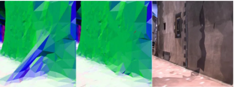
Fig. 1. A visual artifact (left) and its removal (middle and right). The triangle orientations are colored (white: ground, red-green-blue: vertical, black: sky).
constraints. A ray is defined as a line segment between a camera and a point observed by this camera. A tetrahedron is free-space if it is intersected by at last one ray.
The list of triangles separating free-space and matter can, at first glance, be directly considered as the output surface, but the resulting surface is not guaranteed to be a manifold. To enforce the topology constraint, a region growing approach as in [6] can be used, but alone it is limited to genus 0 surfaces. So methods [1], [2] expand it by a topology extension step.
However, the region growing and topology extension steps alone suffer from a visual artifacts problem as illustrated on Fig. 1. The artifact that connects the wall of the building to the ground on the left part of the figure does not exist in reality and should be removed as shown on the central part. This is only one example of situations when the problem arise. It can also occur in other contexts [7].
There were several previous attempts to solve this problem. First of all, computational geometry only approaches [8], [9] that use scanner data consider that spurious handles (a particular, but very usual kind of artifact) are usually small by contrast to the real world handles that would be large. Unfortunately this is not always true in our case. Another idea [1] is to use the visibility information provided by SfM.
The artifact removal method in Sec. 4 of [1] is efficient in terms of resulting surface quality, but, unfortunately, it is the slowest part of the calculation if the input is large enough. Another limitation is the fact that this algorithm has an artificial (Steiner) points addition step that breaks Delaunay property of the triangulation. Although this is not really a problem in the batch case [1], this is not recommended in the incremental framework [2] where the triangulation is updated by vertex additions after every artifact removal step.
Indeed, the Delaunay triangulation has theoretical warranties for surface reconstruction in both geometric [10] and topolog-ical [11] senses. We also benefit by the fast and incremental 3D Delaunay triangulation in the CGAL library [12].
The main contribution of this paper is two other visual artifacts removal methods that are faster than the previous one and don’t require Steiner points addition. Another contribution is a comparison between these methods applied in the incre-mental [2] framework.
Sec. II summarizes the batch and incremental surface reconstruction methods. We remind previous visual artifacts removal method in Sec. III-A and then explain in detail the two new methods proposed by this paper in the remaining of Sec. III. Finally, we compare these methods in Sec. IV.
II. SUMMARY OF SOLID MODELING METHODS
In this section, we summarize the batch and incremental solid modeling methods. The first and common step of the two algorithms is Harris points extraction and their 3D reconstruc-tion by a Structure-from-Moreconstruc-tion algorithm. Let P be a set of 3D points reconstructed by SfM, C a list of camera locations. Let R be the list of rays defined as follow: ∀ci∈ C, ∀pj ∈ P ,
segment cipj∈ R if and only if ci has observed pj.
A. Batch surface reconstruction method
Here is a brief overview of the batch method in [1]. First of all, a 3D Delaunay triangulation T of P is constructed (T is a list of tetrahedra). For all ∆ ∈ T , we define I(∆) as the number of intersections between ∆ and the segments of R. Each tetrahedron ∆ ∈ T is labeled free-space or matter: ∆ is free-space if and only if I(∆) 6= 0. We compute the list F ⊆ T of the free-space tetrahedra.
As the next step, we define another partition of T . Let O ⊆ F such as the border ∂O of O is 2-manifold (∂O is the list of triangles which are faces of exactly one tetrahedron in O). The tetrahedra in O are outside and the others are inside. Initially O = ∅. We begin by the region growing step: for each ∆ ∈ F , we add ∆ to O if ∂O remains manifold. This property is checked using a very fast test. We begin by adding tetrahedra with highest I(∆). This way, we begin by adding tetrahedra with a highest chance of being free-space.
Then, we use the topology extension step to allow the genus of the resulting surface be higher than zero. We add the tetrahedra ∆ ∈ F by packs of tetrahedra incident to a common vertex v ∈ P . To ensure the manifold property, in this configuration, a slower but more general test is used.
We repeat these two steps until no more tetrahedra can be added to O. The resulting surface is the border ∂O of O. Some post-processing steps are then applied to achieve better surface quality (more details in [1]), including the artifact removal method which is summarized in Sec. III-A for paper clarity.
B. Incremental surface reconstruction method
To experiment our artifacts removal methods in an incre-mental context, we use the algorithm described in [2].
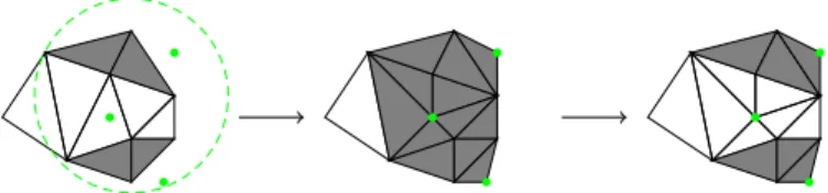
Fig. 2. Incremental reconstruction method overview. White tetrahedra are free-space, gray tetrahedra are matter, green dots are newly added points and green dashed circle is B.
Let Ptbe the set of points computed at time t that will not
be modified by SfM after t (p ∈ Ptand cip ∈ R imply i ≤ t;
i = t exists). At the keyframe/time t + 1, the algorithm has the following input: Ttis a 3D Delaunay triangulation of Pt,
Ft⊆ Tt is a list of free-space tetrahedra of Tt and Ot ⊆ Ft
is a list of outside tetrahedra such that ∂Otis a 2-manifold.
The goal of the algorithm is to update the surface with a set of new SfM points Pt+1. They can not directly be added into
the triangulation Tt because this can modify Ot and break
the manifold property of its border. So we compute a ball B centered on ct+1 with the radius big enough to enclose
Pt+1and neighboring tetrahedra (see Fig. 2). Then we remove
tetrahedra from Ot one-by-one and by packs in the similar
manner than Sec. II-A until ∂Otis still a manifold and we get
as close as possible to Ot∩ B = ∅. This is the shrinking step.
As the next step, we safely add Pt+1 into Tt without
modifying Ot. We obtain Tt+1. Then, we update the
free-space/matter status of tetrahedra and obtain Ft+1⊆ Tt+1.
Finally, to compute the new surface, we initialize Ot+1=
Ot and we apply the region growing and topology extension
algorithms described in Sec. II-A. To enhance the resulting surface quality, some post-processing steps are applied locally to the updated region (see [2] for details).
III. VISUAL ARTIFACTS REMOVAL METHODS
Before we begin the discussion about different artifacts removal methods, we should precisely define what we seek to remove. Using the definitions in Sec. II, the 3D Delaunay triangulation T is encoded by an adjacency graph ΓT in which
the nodes are the tetrahedra of T and the edges are the triangles between two tetrahedra. In the same manner, for any set S ⊆ T of tetrahedra, ΓS ⊆ ΓT is the corresponding adjacency graph.
We define a visual artifact A by A ⊆ F \ O and ΓA is
connected, i.e. a set of tetrahedra that is included in the inside volume (A ∩ O = ∅), but not in the scene matter (A ⊆ F ). Unfortunately, detecting all the artifacts in the resulting model using this definition alone would be too slow to be useful in practice. So we define a visually critical edge [1] as a segment ab such as a ∈ P, b ∈ P and ∃c ∈ C such as cacb > α where α is a user defined threshold (α = 5 deg in this paper). Then, we define a visually critical artifact as a visual artifact which has (at least) a tetrahedron containing a visually critical edge. The artifacts removal methods discussed in this section seek to remove as many visually critical artifacts as they can. We do not use the term spurious handle as in [1], because it is too restrictive. Our algorithms deal with more than just “handles”.
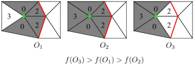
3 0 2 2 0 O1 3 0 2 2 0 O2 3 0 2 2 0 O3 f (O3) > f (O1) > f (O2)
Fig. 3. Escape from local extremum thanks to our new artifacts removal (2D case). White tetrahedra are outside, gray tetrahedra are inside. The number in tetrahedron ∆ is I(∆). The green dot is the vertex considered by the algorithm and thick red lines are critical edges. Left: O before removal. Middle: force neighboring tetrahedra out of O. Right: local growing of O.
A. Summary of previous method
In this section, we briefly discuss the visual artifacts removal method described in [1]. As its entry, this algorithm takes the list Eαof the visually critical edges.
First of all, the method splits each edge of Eαin its middle
by adding a Steiner point (i.e. artificial point which wasn’t seen by any camera). Each edge is split into two parts and the resulting edges are stored in a list Esplit. Each tetrahedron
including the edge is also split in two and the two resulting tetrahedra are assigned the same number of intersections and status as the initial one.
This way, we reduce the size of tetrahedra and hope to locally unlock region growing in the neighborhood of this edge. Furthermore, ∂O is still manifold. The drawback is that the triangulation is not guaranteed to be Delaunay anymore.
After this first step, we create a list Veof the end vertices
of the edges of Esplit. For each vertex v ∈ Ve, we apply a
force/repair cycle as following.
We begin by the force step. Let Lv be the list of the
tetrahedra incident to v. We define G = (Lv ∩ F ) \ O. So
G is a set of tetrahedra forming a visual artifact. We force them into outside: O ← O ∪ G. If the border of O remains manifold, we get what we wanted. If it doesn’t, it contains some vertices whose neighborhood is not topologically a disk. These vertices are called singular vertices in the remaining of this paper. We call n the number of these singular vertices. So, we try to repair O using the next step.
Then, we execute the repair step. We seek to add a bunch of free-space tetrahedra to O such that ∂O become manifold once again. To achieve this goal, we apply a local region growing algorithm to O in F starting in the neighborhood of G and which decreases n. The algorithm stops if a number of iterations g0 (fixed by the user) has been reached or no
more tetrahedra can be added to O. If the repair step succeeds (i.e. n = 0: ∂O is manifold), we was able to remove a visual artifactand proceed to the next vertex. Otherwise, we restore O to the previous state.
B. New visual artifacts removal method
As was previously noted, the method in Sec. III-A is good to improve the surface quality, but unfortunately it has two problems. The first is the need of Steiner points for good results, which break the Delaunay property of the triangulation.
The second problem is that artifacts removal method is slow (48%-72% of the total processing time according to Tab. 2 of [1]). So, we propose a faster visual artifacts removal method that doesn’t require these Steiner points.
The region growing described in Sec. II is a greedy optimization algorithm that maximizes
f (O) = X
∆∈O
I(∆) (1)
in the discrete search space of tetrahedra lists O such that O ⊆ F and ∂O is a 2-manifold. In [1], we have a steepest descent heuristic for function −f (O) (by region growing of O) which can get stuck to a local maximizer of f (O). A visual artifact(e.g. spurious handle) can be seen in this situation. The basic idea of our new method is to remove some tetrahedra from O (and so to decrease f (O)) to kick the algorithm out of its local extrema.
As in the previous section, we call Eα the list of visually
critical edges. Let Gα ⊆ F such that every ∆ ∈ Gα has an
edge in Eα. Then, for every vertex v of both ∂O and Gα, we
force neighboring tetrahedra out of O and we try local region growing beginning from neighboring tetrahedra included in Gα. If the final value of f (O) is greater than the initial one, we
are able to escape from a local maximum, otherwise we revert everything to the initial state and try another vertex v. See Fig. 3 for an example and the algorithm below. Once we tried all ∂O vertices, we complete the result using region growing and topology extension (Sec. II-A) restricted to the tetrahedra included in B (Sec. II-B).
The algorithm in pseudo-code is as follow:
1: function REGION GROWING(∆0)
. Local region growing in Gα
2: Let Q be a priority queue of tetrahedra based on I(∆)
3: PUSH(Q, ∆0)
4: Ladd← ∅
5: while Q 6= ∅ do 6: ∆ ←POP(Q)
7: if ∆ /∈ O and ∂(O ∪ {∆}) is manifold then
8: O ← O ∪ {∆}
9: Ladd← Ladd∪ {∆}
10: for all ∆0 neighbor of ∆ do
11: if ∆0∈ Gα and ∆0∈ O then/ 12: PUSH(Q, ∆0) 13: end if 14: end for 15: end if 16: end while 17: return Ladd 18: end function
19: procedure ARTIFACTS REMOVING
. The main artifacts suppression algorithm
20: sold, s ← 0
21: repeat
22: sold← s
23: for all vertex v of both ∂O and Gα do
24: Nv← all the tetrahedra incident to v
25: Lsub← O ∩ Nv
26: Lseed← (Gα∩ Nv) \ O
1 2 3
Fig. 4. An example of application of spurious handle removal (in the 2D case). White tetrahedra are outside, gray tetrahedra are inside, light gray tetrahedra are freespace inside. The thick blue line is a visually critical edge, the dashed red line is plane π and red dashed triangles are selected tetrahedra.
28: O ← O \ Lsub . Local shrinking
29: if ∂O is manifold then
30: for all ∆ ∈ Lseed do . Local growing
31: Ladd← Ladd∪ REGION GROWING(∆)
32: end for
33: Rsub←P∆∈LsubI(∆) 34: Radd←P∆∈LaddI(∆) 35: if Rsub> Radd then
36: O ← O \ Ladd 37: O ← O ∪ Lsub 38: else 39: s ← s + Radd− Rsub 40: end if 41: else 42: O ← O ∪ Lsub 43: end if 44: end for 45: until sold6= s 46: end procedure
C. New spurious handle removal method
We also propose a visual artifacts removal algorithm that is a specialization of Sec. III-A method. The latter is slow mainly because it consists in many attempts to remove a small pack of tetrahedra and the majority of these attempts are unsuccessful. So, the idea is to remove bigger packs of tetrahedra by placing ourselves in a less general context.
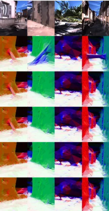
Instead of trying to remove all the visually critical artifacts, we seek to remove a particular kind of artifact: the handle. The fourth column of Fig. 6 shows an example. This is the most visible kind of artifact for the human eye.
The basic idea of the algorithm is to remove the handle (by contrast to Sec. III-A where we remove all the tetrahedra including a vertex) and then try to restore the manifold property of O by a local region growing. To do that, we begin as usual, by computing the list Eα of visually critical edges.
For each edge ab ∈ Eα, we check if it is contained in a handle.
We define a plane π perpendicular to ab and intersecting segment ab in some point. In practice we try several planes intersecting ab in 2a+b3 , a+b2 and a+2b3 . Let Lπ be the list
of the tetrahedra intersected by π. Let Nab be the list of the
tetrahedra including edge ab. A handle H is a set of tetrahedra forming a visual artifact, so H ⊆ F \ O. With this definition, we begin to form our handle by H ← (Nab∩ Lπ∩ F ) \ O.
Let NHbe the list of the tetrahedra directly adjacent to the
set H (i.e. ∀∆ ∈ NH, ∆ has a 4-neighbor in H). We iteratively
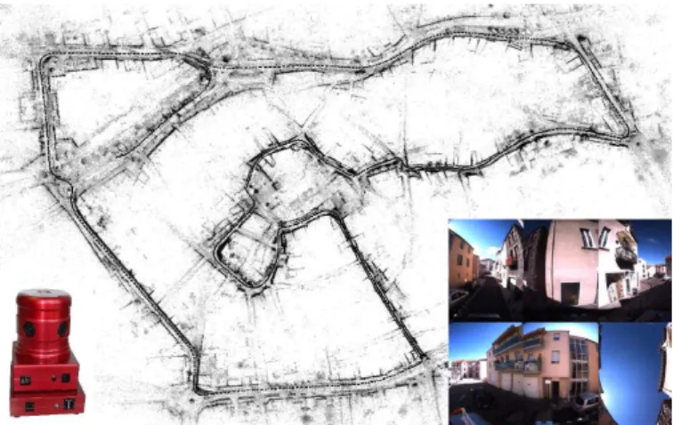
Fig. 5. Global overview of the SfM points cloud of our test trajectory as well as an example of the Ladybug camera image.
grow H by performing H ← H ∪ ((NH ∩ Lπ ∩ F ) \ O)
until no more tetrahedra can be added. Then we check that the final H is surrounded by O in plane π (see Fig. 4), i.e. ∀∆ ∈ (NH∩ Lπ) \ H, ∆ ∈ O.
Once we have detected a handle H, we try to remove it as in Sec. III-A. First we force H in O (i.e O ← O ∪H), then we try to restore the 2-manifold property of ∂O using the repair step initialized by the tetrahedra in (NH∩F )\O. If we succeed,
we remove an artifact, otherwise we undo everything and try another edge in Eα.
IV. EXPERIMENTS
A. Dataset
To perform a quantitative evaluation of the visual artifacts removal methods discussed in this paper, we use the SfM dataset in [2]. The video is a 2.5 km. long trajectory taken in a general urban environment by a PointGrey Ladybug omnidirectional camera. Our SfM is based on local bundle adjustment [13] and is refined by a global bundle adjustment to close the large loop (2.3 km). The SfM selects 1306 keyframes out of 7735 frames and detects 2.64M Harris interest points. 483k 3D points are reconstructed and shown in Fig. 5. Thus, we only have 193 points per meter to reconstruct the surface.
B. How to compare the artifact removal methods ?
Every removal method is integrated in the surface post-processing step of the incremental surface reconstruction method [2] (before smoothing). To compare the methods in terms of output surface quality, we manually count the visually critical artifacts (Sec. III) remaining on the final surface. Because we seek to remove in priority the artifacts that are visually critical (and so are easily noticed by a human eye), we consider this number as a good quantitative metric. Fig. 6 shows examples of artifacts that are manually counted. Moreover, we also estimate the final number of freespace inside tetrahedra (i.e. the union of the visual artifacts) and the final value of the objective function f (Eq. 1). The latter quantifies the ability of every method to unlock region growing and topology extension steps (Sec. II-A), or in other words, the ability to escape from local extremum of f .
Fig. 6. Results of artifacts removal methods at four locations (one location per column). Lines from top to bottom: textured scene, no artifacts removal, method III.A, method III.B, method III.C, method III.B&C.
C. Comparisons
We evaluate five visual artifacts removal methods: None (no removal method), III.A (the method in [2] summarized in Sec. III-A), III.B (escape from local extremum using the method in Sec. III-B), III.C (handle removal using the method in Sec. III-C), III.B&C (use III.C after III.B). The results are summarized in Tab. I. The removal methods III.A, III.B, III.C and III.B&C provide similar improvements (increases) of the objective function f . The differences between them are small (less than 0.034%), but we see that III.A is slightly better than III.B and III.C taken separately. Furthermore, we see that the combination of III.B and III.C is slightly better than III.A,
TABLE I. ARTIFACTS REMOVAL RESULTS
Removal Mean Max. Num. Size of f= P
∆∈O
I(∆) Num.
method time time artif. F \ O (M = 106) tests None 0 0 20 139448 29.822M 0 III.A 1.1 s. 3.87 s 16 93259 30.012M 468M III.B 0.33 s. 0.94 s 18 92604 30.009M 186M III.C 0.27 s. 0.99 s 15 94469 30.002M 136M III.B&C 0.43 s. 1.2 s 13 92280 30.013M 323M 0 0.5 1 1.5 2 2.5 3 3.5 4 0 200 400 600 800 1000 1200 1400 Ti m e (s ) Key frame Computation times comparison
III.A III.B & III.C
Fig. 7. Computation times at every keyframe for both previous (III.A, red) and new (III.B&C, green) visual artifact removal methods.
and this is confirmed by both the number of tetrahedra in F \ O (union of all visual artifacts) and the number of artifacts that are manually detected. Fig. 6 compares the results of all methods at four locations in the reconstruction and is consistent with these comparisons. We note that III.B has important visual artifacts (as the one in the left of this figure) although it has a good (small) F \ O, and III.C can correct them in spite of its greater F \ O. Then we think that the combination III.B&C is a good choice.
A difference between the four methods is the calculation time. Indeed, III.B, III.C and III.B&C are significantly faster than III.A since their mean time per keyframe is about 2.5-4 times smaller (Tab. I and Fig. 7). We also see that III.A needs the largest number of tests that check the manifold property at a vertex.
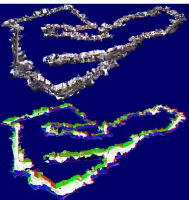
D. More details on III.B&C Result
Fig. 8 shows a global view of the 3D models reconstructed by the method in [2] including the artifact removal method III.B&C. At the end of the process, the surface has 600k triangles and the 3D Delaunay has 2.09M tetrahedra. The computation times for every keyframe is in Fig. 9. We use a 4xIntel Xeon W3530 at 2.8Ghz. The surface reconstruction time for every keyframe has mean 1.87 s. and maximal value 5.39 s. The largest times are at the sequence end, where the large loop is closed. As in [2], this is due to the fact that we reconstruct new points of the loop end at a location where points are already reconstructed at the loop beginning. The joint video shows the progressive surface reconstruction and the final surface.
We observe differences with [2]: the artifact removal step (previously named handle removal) is not the most costly step anymore, and the global times are roughly divided by 1.5-2.
Fig. 8. Global overview of the final surface obtained by our incremental surface reconstruction method including III.B&C as visual artifact removal. We show a textured view (top) and color coded normals (bottom). The triangles on the sky are removed for visualization purposes.
0 1 2 3 4 5 6 7 0 200 400 600 800 1000 1200 1400 Ti m e (s ) Key frame Time statistics Artifacts removal Artifacts detection Post-processing Grow Ray tracing Triangulation Shrink
Fig. 9. Computation times at every keyframe for the steps of our incremental surface reconstruction method including III.B&C as visual artifact removal. Note that these times are accumulated for steps shrink, . . . , artifact removal.
These improvements are the consequences of both our artifact removals (our contribution) and reasons in the Appendix.
V. CONCLUSION
This paper improves the visual artifact removal step of a recent incremental method which reconstructs a 2-manifold surface from sparse Structure-from-Motion data. We replace this step by the same method restricted on particular cases of visual artifacts (handles) and preceded by another method which escapes from the local extrema of the objective function. Then the processing time of the step is greatly reduced without loss of surface quality. We experiment on a 2.5km. long video sequence taken by an omnidirectional camera moving in an
urban environment.
Future work includes improvements of calculation time and surface quality, e.g. reconstruct and integrate the image contours in the 3D Delaunay triangulation, improve the interest point matching, investigate other objective cost functions.
REFERENCES
[1] M. Lhuillier and S. Yu, “Manifold surface reconstruction of an envi-ronment from sparse Structure-from-Motion data,” Computer Vision and Image Understanding, vol. 117, no. 11, pp. 1628–1644, 2013. [2] V. Litvinov and M. Lhuillier, “Incremental solid modeling from sparse
and omnidirectional Structure-from-Motion data,” in Proc. British Ma-chine Vision Conference (BMVC), 2013.
[3] Q. Pan, G. Reitmayr, and T. Drummond, “ProFROMA: Probabilistic feature-based on-line rapid model acquisition,” in Proc. British Machine Vision Conference (BMVC), 2009.
[4] D. Lovi, N. Birkbeck, D. Cobzas, and M. Jagersand, “Incremental free-space carving for real-time 3D reconstruction,” in Proc. 3D Imaging, Modeling, Processing, Visualization, Transmission (3DIMPVT), 2012. [5] C. Hoppe, M. Klopschitz, M. Donoser, and H. Bischof, “Incremental
surface extraction from sparse Structure-from-Motion point clouds,” in Proc. British Machine Vision Conference (BMVC), 2013.
[6] O. Faugeras, E. Le Bras Mehlman, and J. Boissonnat, “Representing stereo data with the Delaunay triangulation,” Artificial Intelligence, pp. 41–47, 1990.
[7] R. Chaine, “A geometric convection approach of 3D reconstruction,” Eurographics Symposium on Geometry Processing, pp. 218–229, 2003. [8] Z. Wood, H. Hoppe, M. Desbrun, and P. Shr¨oder, “Removing excess topology from isosurfaces,” ACM Transactions on Graphics (TOG), vol. 23(2), pp. 190–208, 2004.
[9] Q. Zhou, T. Ju, and S. Hu, “Topology repair of solid models using skeletons,” IEEE Transactions on Visualization and Computer Graphics, vol. 13(4), pp. 675–685, 2007.
[10] J. Boissonnat and S. Oudot, “Provably good sampling and meshing of surfaces,” Graphical Models, vol. 67, no. 5, pp. 405–451, 2005. [11] N. Amenta and M. Bern, “Surface reconstruction by Voronoi filtering,”
Discrete Computational Geometry, vol. 22, no. 4, pp. 481–504, 1999. [12] CGAL, “Computational Geometry Algorithms Library,” www.cgal.org. [13] E. Mouragnon, M. Lhuillier, M. Dhome, F. Dekeyser, and P. Sayd, “Generic and real-time Structure-from-Motion,” in Proc. British Ma-chine Vision Conference (BMVC), 2007.
APPENDIX
Corrections are applied to the implementation in [2]. An implementation bug is corrected and the shrinking step is now slower but more accurate than before. We remember that the ideal result of shrinking meet O ∩ B = ∅ where B is a ball where almost all computations are done. Now this condition is not meet in only one of the 1306 keyframes (before: 4.5% of the keyframes). As a consequence, the step of the regular Steiner points grid can be reduced to 10 times mean distance between consecutive camera locations (before: 15 times). We remember that this grid is useful to reduce the size of B and these Steiner points do not break Delaunay property [2].
Moreover, the topology extension step of shrinking and growing is re-implemented in a multi-threaded fashion. As was briefly explained in Sec. II, this step consists mainly in trying to add or remove a pack of tetrahedra to the outside region. In the new implementation, we simply perform many tests simultaneously, so these steps are greatly accelerated.
ACKNOWLEDGEMENTS