HAL Id: hal-00150283
https://hal.archives-ouvertes.fr/hal-00150283
Preprint submitted on 30 May 2007
HAL is a multi-disciplinary open access
archive for the deposit and dissemination of
sci-entific research documents, whether they are
pub-lished or not. The documents may come from
teaching and research institutions in France or
L’archive ouverte pluridisciplinaire HAL, est
destinée au dépôt et à la diffusion de documents
scientifiques de niveau recherche, publiés ou non,
émanant des établissements d’enseignement et de
recherche français ou étrangers, des laboratoires
Classical F_omega, orthogonality and symmetric
candidates
Stéphane Lengrand, Alexandre Miquel
To cite this version:
Stéphane Lengrand, Alexandre Miquel. Classical F_omega, orthogonality and symmetric candidates.
2007. �hal-00150283�
Classical F
ω
,
orthogonality and symmetric candidates
Stéphane Lengrand
1,2and Alexandre Miquel
1 1PPS & Université Paris 7
175 rue du Chevaleret, 75013 Paris, France
2
School of Computer Science, University of St Andrews
North Haugh, St Andrews, Fife, KY16 9SX, Scotland
Abstract We present a version of system Fω, called F
C
ω, in which the layer of type
constructors is essentially the traditional one of Fω, whereas provability
of types is classical. The proof-term calculus accounting for the classical reasoning is a variant of Barbanera and Berardi’s symmetric λ-calculus.
We prove that the whole calculus is strongly normalising. For the layer of type constructors, we use Tait and Girard’s reducibility method combined with orthogonality techniques. For the (classical) layer of terms, we use Barbanera and Berardi’s method based on a symmetric notion of reducibility candidate. We prove that orthogonality does not capture the fixpoint construction of symmetric candidates.
We establish the consistency of FC
ω, and relate the calculus to the
traditional system Fω, also when the latter is extended with axioms for
classical logic.
1
Introduction
Approaches to a Curry-Howard correspondence for classical logic seem to con-verge towards the idea of programs equipped with some notion of control [Par92, BB96, Urb00, Sel01, CH00]. The general notion of reduction/computation is non-confluent but there are possible ways to restrict reductions and thus re-cover confluence.1
It is then tempting to try and build, on such a correspondence for classical logic, powerful type theories, such as those developed in intuitionistic logic (Pure Type Systems [Bar91, Bar92], Martin-Löf type theories [ML84]). Approaches to this task (in natural deduction) can be found in [Ste00], in a framework à la Martin-Löf, and in [BHS97] (but with a confluent restriction of the reductions of classical logic).
1
Two such canonical ways are related to CBV and CBN, with associated semantics given by CPS-translations, which correspond to the usual encodings of classical logic into intuitionistic logic known as “not-not”-translations.
Intuitionistic type theories, however, exploit the fact that predicates are pure functions, which, when fully applied, give rise to formulae with logical meanings. The Curry-Howard correspondence in intuitionistic logic can then describe these pure functions as the inhabitants of implicative types in a higher type layer (often called the layer of kinds).
On the other hand, inhabitants of implicative types in classical logic can be much wilder than pure functions (owing to the aforementioned notion of control), so it is not clear what meaning could be given to those simili-predicates, built from classical inhabitants of implicative types, and whose reductions may not even be confluent. However, such an issue is problematic only in the layer of types, a.k.a the upper layer, which various type theories “cleanly” separate from the layer of terms, a.k.a the lower layer.
This paper, which extends [LM06], shows that it is perfectly safe to have cohabiting layers with different logics, provided that the layer of types is free from any dependency on terms, i.e. that the system has no dependent types. For that we chose to tackle System Fω [Gir72]. We present here a version of it
called FC
ω that is classical in the following sense:
The upper layer is purely functional, i.e. intuitionistic: it is in fact the lambda-calculus extended with constants for logical connectives. Then, for those objects of the layer that are types (a.k.a. formulae), we have a notion of provability with proof derivations and proof-terms in the lower layer, which is here classical instead of intuitionistic.
The motivation for the choice of tackling Fω is threefold:
• System Fωis indeed the most powerful corner of Barendregt’s Cube
with-out dependent types [Bar91, Bar92].
• System F and the simply-typed λ-calculus also cleanly separate the lower layer from the upper layer, but the latter is trivial as no computation happens there, in contrast to System Fω which features computation in
both layers, both strongly normalising. • The version FC
ω with a classical lower layer, in contrast to the intuitionistic
one, features two different notions of computation (one intuitionistic and confluent, the other one classical and non-confluent), also both strongly normalising. Hence, FC
ω represents an excellent opportunity to express
and compare two techniques to prove strong normalisation that are based on the method of reducibility of Tait and Girard [Gir72] and that look very similar, and solve a conjecture raised in [LM06] about one technique not capturing the other.
The strong normalisation of the upper layer (section 3.1) represents an op-portunity to rephrase the reducibility method [Gir72] with the concepts and terminology of orthogonality, which provides a high level of abstraction and potential for modularity, but has a sparse literature (which includes [MV05]).
The technique for the strong normalisation of the lower layer (section 3.2) adapts Barbanera and Berardi’s method based on a symmetric notion of re-ducibility candidate [BB96] and a fixpoint construction. Previous works (e.g.
[Pol04, DGLL05]) adapt it to prove the strong normalisation of various sequent calculi, but (to our knowledge) not pushing it to such a typing system as that of FC
ω (with a notion of computation on types). Note that we also introduce
the notion of orthogonality in the proof technique (to elegantly express it and compare it to the proof for the upper layer).
The method works in fact without any surprise. Difficulties would come with dependent types (the only feature of Barendregt’s Cube missing here), precisely because they would pollute the layer of types with non-confluence and unclear semantics.
The main purpose of presenting together the two proof techniques described above is in fact to express them whilst pointing out similarities, and to exam-ine whether or not the concepts of the symmetric candidates method can be captured by the concept of orthogonality. In this paper we solve the conjecture of [LM06] by proving that it cannot.
Finally we prove the consistency of FC
ω, and establish a formal connection
with the traditional system Fω, also when the latter uses extra axioms to allow
classical reasoning.
Section 2 introduces FC
ω. Section 3 establishes the strong normalisation of
the layer of types, and that of the layer of terms. Section 4 compares the two proofs and solves the conjecture of [LM06]. Section 5 establishes some logical properties of Fωsuch as consistency.
2
Syntax, Reduction and Typing of F
ωC2.1
Syntax
FC
ω distinguishes four syntactic categories: kinds, type constructors (or
construc-tors for short), terms and programs: Kinds Constructors Terms Programs K, K′ ::= ⋆ | K → K′ A, B, C, . . . ::= α | α⊥ | λα : K . B | B A | A ∧ B | A ∨ B | ∀α : K . B | ∃α : K . B t, u, v, . . . ::= x | µxA.p | ht, ui | λxAyB.c | Λα : K . t | hA, ti p ::= {t | u}
Kinds, that are exactly the same as in system Fω[Gir72, BG01], are a system of
simple types for type constructors. (We use the word ‘kind’ to distinguish kinds from the types which appear at the level of type constructors.) The basic kind ⋆ is the kind of types, that is, the kind of all type constructors that represent types of terms—or propositions/formulae through the Curry-Howard correspondence. Type constructors, often shortened as constructors, are basically simply-typed λ-terms with two binary operators A ∧ B (conjunction), A ∨ B
(dis-junction) and two extra binders ∀α : K . A and ∃α : K . A to represent universal and existential quantification. (There is no primitive implication in the system.) As in linear logic [Gir87], negation α 7→ α⊥ is only primitive on variables,
but the extension as an involution A 7→ A⊥ on all type constructors is defined
via de Morgan laws:
(α)⊥ = α⊥ (α⊥)⊥ = α (A ∧ B)⊥ = A⊥∨ B⊥ (A ∨ B)⊥ = A⊥∧ B⊥ (∀α : K . B)⊥ = ∃α : K . B⊥ (∃α : K . B)⊥ = ∀α : K . B⊥ (λα : K . B)⊥ = λα : K . B⊥ (B A)⊥ = B⊥A
Notice how negation propagates through λ-abstraction and application. In our calculus, the notation A⊥ is not only meaningful for types (that is, constructors
of kind ⋆), but it is defined for all type constructors.
With negation extended to all type constructors we can define implication A ⇒ B as (A⊥) ∨ B.
However, one must take care in the way constructor variables are bound. In what follows, we assume that the constructions ∀α : K . B, ∃α : K . B and λα : K . B bind all free occurrences of the variable α in B, including those which correspond to a subterm of the form α⊥. (In other words, the syntactic
con-struction α⊥ is not a variable.) For instance, the type constructor
¬ = λα : ⋆ . α⊥
is closed; this is the type constructor which represents negation as a function (of kind ⋆ → ⋆). The computation rules of negation are incorporated into the calculus by extending the definition of the (external) operation of substitution written B{α\A} to the case where B is a negated variable, as shown in Fig. 1.
(λα : K . A){β\C} = λα : K . A{β\C} α{β\C} = α (if β 6= α) β{β\C} = C α⊥{β\C} = α⊥ (if β 6= α) β⊥{β\C} = C⊥ (A ∧ B){β\C} = A{β\C} ∧ B{β\C} (A ∨ B){β\C} = A{β\C} ∨ B{β\C} (∀α : K . A){β\C} = ∀α : K . A{β\C} (∃α : K . A){β\C} = ∃α : K . A{β\C}
This (extended) notion of substitution satisfies the following properties: Remark 1
1. (A{α\B})⊥= A⊥{α\B}.
2. A{α\B}{β\C} = A{β\C}{α\B{β\C}}
The (proof-)terms of our calculus are basically the terms of Barbanera and Berardi’s symmetric λ-calculus, with the difference that connectives are treated multiplicatively. In particular, disjunction is treated as a negative connective whose proofs are built using a double binder written λxAyB.p. On the other
hand, proofs of conjunction are introduced as usual, using the pairing construct written ht, ui.
Finally, programs are built by making two terms t and u interact using a construction written {t | u}, where each term can be understood as the evalua-tion context of the other term. We assume that this construcevalua-tion is symmetric, that is, that {t | u} and {u | t} denote the same program. Henceforth, terms and programs are considered up to this equality together with α-conversion.
2.2
Reduction and Typing for Types
The reduction relation on the layer of type constructors is β-reduction, which is defined as usual as the contextual closure of the relation
(λα : K . B)A −→β B{α\A} .
However, the extension of the definition of substitution to negated variables me-chanically enhances β-reduction in such a way that we get de Morgan equalities for free:
¬(A ∧ B) =β ¬A ∨ ¬B ¬(A ∨ B) =β ¬A ∧ ¬B
¬(∀α : K . B) =β ∃α : K . ¬B ¬(∃α : K . B) =β ∀α : K . ¬B
(Here, ¬ denotes the type constructor λα : ⋆ . α⊥, and =
βdenotes the symmetric
transitive and reflexive closure of −→β.)
Proposition 2 — The (enhanced) β-reduction on type constructors is conflu-ent.
Proof: This is proved by introducing the corresponding notion of parallel reduction, following Tait and Martin-Löf [Bar84]. ✷
(α : K) ∈ Σ Σ ⊢ α : K Σ ⊢ α⊥: K (α : K) ∈ Σ Σ, α : K ⊢ B : K′ Σ ⊢ λα : K . B : K → K′ Σ ⊢ B : K → K′ Σ ⊢ A : K Σ ⊢ B A : K′ Σ ⊢ A : ⋆ Σ ⊢ B : ⋆ Σ ⊢ A ∧ B : ⋆ Σ ⊢ A : ⋆ Σ ⊢ B : ⋆ Σ ⊢ A ∨ B : ⋆ Σ, α : K ⊢ B : ⋆ Σ ⊢ ∀α : K . B : ⋆ Σ, α : K ⊢ B : ⋆ Σ ⊢ ∃α : K . B : ⋆
Figure 2: Typing rules for type constructors
Typing contexts for variables of type constructors, that we call signatures, are (unordered) lists of declarations of the form (α : K):
Signatures Σ ::= α1: K1, . . . , αn: Kn
The inference rules of the typing judgement Σ ⊢ A : K (‘In the signature Σ, A is a constructor of kind K’) are given in Fig. 2.
The typing system satisfies the following properties:
Proposition 3 1. (Weakening) If Σ ⊢ A : K then Σ, α : K′ ⊢ A : K.
2. (Negation preserves typing) If Σ ⊢ A : K then Σ ⊢ A⊥: K.
3. (Substitution is well-typed) If Σ ⊢ A : K and Σ, α : K ⊢ B : K′ then
Σ ⊢ B{α\A} : K′.
It also satisfies Subject reduction:
Proposition 4 (Subject reduction) — If Σ ⊢ A : K and if A −→β A′,
then Σ ⊢ A′ : K.
2.3
Reduction and Typing for Terms and Programs
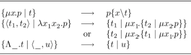
The reduction system of the lower layer of FC
ω, presented in Fig. 3, applies on
programs, but the contextual closure equip both programs and terms with a reduction relation. Recall that the programs {t | u} and {u | t} are identified, so we consider the reduction relation modulo the congruence defined by this identity and we denote it −→FC
{µxA.p | t} −→ µ p{x\t} {ht1, t2i | λxA1xB2.p} −→∧∨l {t1| µx A 1.{t2| µxB2.p}} or −→∧∨r {t2| µx B 2.{t1| µxA1.p}}
{Λα : K . t | hA, ui} −→∀∃ {t{α\A} | u}
Figure 3: Reduction rules on terms and programs
As in Barbanera and Berardi’s symmetric λ-calculus [BB96] or in Curien and Herbelin’s λµ˜µ-calculus [CH00], the critical pair
{µxA.p | µyA′.q}
ւ ց
p{x\µyA′
.q} q{y\µxA.p}
cannot be joined, and in fact reduction is not confluent in general in this layer (see Example 2 below).
Typing contexts for variables of terms, that we simply call contexts, are lists of declarations of the form (x : A):
Contexts Γ ::= x1: A1, . . . , xn: An
Since types A that appear in a context may depend on constructor variables, each context Γ only makes sense in a given signature Σ. In what follows, we say that a context Γ is well-formed in a signature Σ and write wfΣ(Γ) if for all
declarations (x : A) ∈ Γ, the judgement Σ ⊢ A : ⋆ is derivable. From this, we define two judgements, namely:
Γ ⊢Σt : A ‘In the signature Σ and context Γ, the term t has type A’
Γ ⊢Σp ⋄ ‘In the signature Σ and context Γ, the program p is well-formed’
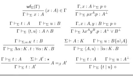
Both judgements are defined by mutual induction from the rules given in Fig. 4. This typing system satisfies the following properties:
Proposition 5 1. (Weakening of signature) If Γ ⊢Σ t : B (resp. Γ ⊢Σ p ⋄)
then Γ ⊢Σ,α : K t : B (resp. Γ ⊢Σ,α : K p ⋄.)
2. (Weakening of context) If Γ ⊢Σt : B (resp. Γ ⊢Σp ⋄) and Σ ⊢ A : K then
Γ, x : A ⊢Σ t : B (resp. Γ, x : A ⊢Σ p ⋄.)
3. (Substitution of constructors is well-typed) If Σ ⊢ A : K and Γ ⊢Σ,α:K t : B
(resp. Γ ⊢Σ,α:K p ⋄) then Γ{α\A} ⊢Σ t{α\A} : B{α\A} (resp.
Γ{α\A} ⊢Σ p{α\A} ⋄).
4. (Substitution of terms is well-typed) If Γ ⊢Σ u : A and Γ, x : A ⊢Σ t : B
wfΣ(Γ) (x : A) ∈ Γ Γ ⊢Σx : A Γ, x : A ⊢Σp ⋄ Γ ⊢ΣµxA.p : A⊥ Γ ⊢Σt : A Γ ⊢Σu : B Γ ⊢Σht, ui : A ∧ B Γ, x : A, y : B ⊢Σ p ⋄ Γ ⊢ΣλxAyB.p : A⊥∨ B⊥ Γ ⊢Σ,α:K t : B Γ ⊢ΣΛα : K . t : ∀α : K . B Σ ⊢ A : K Γ ⊢Σ u : B{α\A} Γ ⊢ΣhA, ui : ∃α : K . B Γ ⊢Σ t : A Σ ⊢ A′: ⋆ A =βA′ Γ ⊢Σt : A′ Γ ⊢Σt : A Γ ⊢Σ u : A⊥ Γ ⊢Σ {t | u} ⋄
Figure 4: Typing rules for terms and programs
And again it also satisfies Subject reduction, despite the non-deterministic nature of reduction: Proposition 6 (Subject-reduction) 1. If Γ ⊢Σt : A and t −→FC ω t ′, then Γ ⊢ Σ t′ : A. 2. If Γ ⊢Σp ⋄ and p −→FC ω p ′, then Γ ⊢ Σ p′ ⋄.
Proof: By simultaneous induction on the judgements Γ ⊢Σt : A and Γ ⊢Σp ⋄.
✷ Example 1 Here is a proof of the Law of excluded middle:
x : α⊥, y : α ⊢α: ⋆x : α⊥ x : α⊥, y : α ⊢α: ⋆y : α x : α⊥, y : α ⊢ α: ⋆{x | y} ⋄ ⊢α: ⋆λxα ⊥ yα.{x | y} : α ∨ (α⊥) ⊢ Λα : ⋆ . λxα⊥yα.{x | y} : ∀α : ⋆ . α ∨ (α⊥)
Example 2 Here is Lafont’s example of non-confluence. Suppose Γ ⊢α: ⋆p1 ⋄
and Γ ⊢α: ⋆ p2 ⋄. With x 6∈ FV(p1) and y 6∈ FV(p2), by weakening we get
Γ, x : α ⊢α: ⋆p1⋄ Γ ⊢α: ⋆ µxα.p1 : α⊥ Γ, y : α⊥ ⊢α: ⋆ p2 ⋄ Γ ⊢α: ⋆ µyα ⊥ .p2 : α Γ ⊢α: ⋆{µxα.p1| µyα ⊥ .p2} ⋄ But {µxα.p 1| µyα ⊥ .p2} −→∗µ p1 or {µxα.p1| µyα ⊥
.p2} −→∗µ p2. And unless the
Note that, in constrast to Barbanera and Berardi’s symmetric λ-calculus, our design choices for the typing rules are such that, by constraining terms and programs to be linear, we get exactly the multiplicative fragment of linear logic [Gir87].
3
Strong normalisation
In this section we prove the strong normalisation of the two layers of FC ω. In
both cases the method is based on the reducibility technique of Tait and Gi-rard [Gir72].
This consists in building a strongly normalising model of the calculus, in-terpreting kinds (resp. types) as sets of strongly normalising type constructors (resp. pairs of strongly normalising terms). By definition, these sets (resp. pairs of sets) contain the basic constructs that introduce a connective (resp. that introduce dual connectives).
This is sufficient to treat most cases of the induction to prove the soundness theorem (which roughly states that being typed implies being in the model, hence being strongly normalising), but for the other cases we need the property that the interpretation of kinds (resp. types) is saturated, so we extend these interpretations by a completion process.
Now the completion process is precisely where the proofs of strong normali-sation of the two layers differ: For the upper layer we simply use a completion by bi-orthogonality and this gives us the desired saturation property. For the lower layer, the completion process is obtained by Barbanera and Berardi’s fixpoint construction. We discuss this difference in section 4.
3.1
Strong normalisation of type constructors
In this section we prove that all well-typed constructors are strongly normal-isable. For that, let us write SNC the set of all strongly normalisable type
constructors.
We call a stack (of type constructors) any finite sequence S = (A1, . . . , An)
of type constructors. Given a type constructor B and a stack S = (A1, . . . , An),
we define the application BS by setting BS = BA1· · · An.
We say that a stack S = (A1, . . . , An) is strongly normalisable when all
its elements A1, . . . , An are strongly normalisable. The set of all strongly
nor-malisable stacks is written SN∗C. In general, applying a strongly normalisable
constructor B ∈ SNC to a strongly normalisable stack S ∈ SN∗C does not yield
a strongly normalisable constructor BS. In the case where BS ∈ SNC, we thus
say that B and S are orthogonal, and write B ⊥ S.
Given a subset X ⊂ SNC, we write X⊥ the subset of SN∗C called the
orthog-onal of X and defined by
X⊥ = {S ∈ SN∗
Similarly, the orthogonal Y⊥⊂ SN
C of a subset Y ⊂ SN∗C is defined as
Y⊥ = {B ∈ SNC | B ⊥ S for all S ∈ Y } .
The operation X 7→ X⊥fulfils the usual properties of orthogonality on SN C
(as well as on SN∗C):
1. X ⊂ X′ entails X′⊥⊂ X⊥ (contravariance)
2. X ⊂ X⊥⊥ (closure)
3. X⊥⊥⊥= X⊥ (tri-orthogonal)
Definition 1 (Reducibility candidate) — We call a reducibility candidate any subset X ⊂ SNC such that X = X⊥⊥.
Notice that reducibility candidates are precisely the subsets X ⊂ SNC of the
form X = Y⊥ for some subset Y ⊂ SN∗
C. In particular, SNC is a reducibility
candidate, since SNC = {()}⊥ (writing () for the empty stack).
Reducibility candidates enjoy the following properties: Proposition 7 — For all reducibility candidates X:
1. X ⊂ SNC;
2. X contains all variables α and negated variables α⊥;
3. X is closed under β-reduction, that is: if B ∈ X and B −→β B′, then B′∈ X;
4. X is saturated, i.e. closed under head β-expansion: if B{α\A} ∈ X and A ∈ SNC, then (λα : K . B)A ∈ X.
Proof: Item 1 holds by definition. Item 2 holds since αS (resp. α⊥S) is
strongly normalisable as soon as the stack S is strongly normalisable. Item 3 holds since strongly normalisable type constructors are closed under β-reduction. Finally, item 4 is a consequence of the following property: If the type construc-tors A and B{α\A}A1· · · An are strongly normalisable, then so is
(λα : K . B)AA1· · · An. ✷
Definition 2 (Set constructions) We define the following abbreviations: X → X′ = {B ∈ SN
C| ∀A∈X, (BA)∈X′}
λX . X′ = {λα : K . B ∈ SN
C | ∀A ∈ X, B{α\A} ∈ X′}
Lemma 8 — For all subsets X ⊂ SNC and Y ⊂ SN∗C,
Proof: Since Y⊥ is a reducibility candidate (Y⊥ = Y⊥⊥⊥), it is
satu-rated, that is, if B{α\A} ∈ Y⊥ then (λα : K . B) A ∈ Y⊥. Hence, we get
λX . Y⊥⊂ X → Y⊥.
Now notice that X → Y⊥= {A :: S | A ∈ X, S ∈ Y }⊥
(where A :: S denotes the consing operation on stacks), so it is a reducibility candidate as well, and thus (λX . Y⊥)⊥⊥⊂ X → Y⊥.
This direction is enough for the proof of strong normalisation, but the reverse direction can also be proved:
Assuming C ∈ X → Y⊥ and S ∈ (λX . Y⊥)⊥, we want to show C ⊥ S.
Since C ∈ SNC and S ∈ SN∗C, any infinite reduction sequence would start with:
C S −→∗β (λα : K . B) S′ with S −→∗ β S′ ∈ (λX . Y⊥) ⊥ and C −→∗ β λα : K . B ∈ (X → Y⊥), for which λα : K . B ∈ λX . Y⊥. ✷ From this, we interpret each kind K as a reducibility candidate:
Definition 3 (Interpretation of kinds) The interpretation [K] of a kind K is a reducibility candidate defined by induction on K as follows:
[⋆] = SNC
[K → K′] = [K] → [K′] = (λ[K] . [K′])⊥⊥
Lemma 9 — If the typing judgment α1: K1, . . . , αn: Kn⊢ B : K is derivable,
then for all A1∈ [K1], . . . , An∈ [Kn] one has
B{α1, . . . , αn\A1, . . . , An} ∈ [K]
(where B{α1, . . . , αn\A1, . . . , An} denotes the parallel substitution of the type
constructors A1, . . . , An to the variables α1, . . . , αn in the type constructor B).
Proof: By induction on the derivation of α1: K1, . . . , αn: Kn⊢ B : K. ✷
From this we get:
Theorem 10 — It Σ ⊢ B : K, then B is strongly normalisable.
Proof: Apply lemma 9 with A1 = α1, . . . , An = αn (identity substitution),
using item 2 of Prop. 7. ✷
3.2
Strong normalisation of terms
This proof is adapted from those of [BB96, Pol04, DGLL05] for the symmetric λ-calculus [BB96], the λµeµ-calculus [CH00], and the dual calculus [Wad03] (which are based on a bi-sided sequent calculi), respectively. They all use Barbanera and Berardi’s symmetric candidates, with a fixpoint construct to capture the non-confluence of classical logic.
As usual with the reducibility method we construct a model of the calculus by interpreting types (here, type constructors and type lists) as sets of terms. However, the second-order quantification that appears in System F or Fω is
conveniently interpreted as a set intersection only if terms do not display type annotations. We therefore start by defining such term and programs, i.e. Curry-style terms and programs:
Curry-style terms t, u, v, . . . ::= x | µx.p | ht, ui | λxy.p | Λ_.t | h_, ti Curry-style programs p ::= {t | u}
The corresponding reduction rules, that are shown in Fig. 5, define the re-ductions −→FC
ω and the set SN of Curry-style terms and Curry-style programs.
{µx.p | t} −→ p{x\t}
{ht1, t2i | λx1x2.p} −→ {t1| µx1.{t2| µx2.p}}
or {t2| µx2.{t1| µx1.p}}
{Λ_.t | h_, ui} −→ {t | u}
Figure 5: Reductions without types
Definition 4 — The type-erasure operation from terms (resp. programs) to Curry-style terms (resp. Curry-style programs) is recursively defined by:
kxk = x
kht, uik = hktk, kuki kλxAyB.pk = λxy.kpk
kµxA.pk = µx.kpk
kΛα : K . tk = Λ_.ktk khA, tik = h_, ktki k{t | u}k = {ktk | kuk}
Note that by erasing the types we still keep, in Curry-style programs, a trace of the constructs introducing the ∀ and ∃ quantifiers. Thus, it is slightly different from the traditional Curry-style polymorphism of system F or Fω, but
this trace turns out to be important in classical logic: if we removed it, we could make some µ-µ critical pair appear that was not present in the original program with type annotations, and one of the two reductions might not satisfy subject reduction.2
2
This is a general problem of polymorphism and classical logic with non-confluent reduc-tion: for instance the spirit of intersection types [CD78], which represent finite polymorphism, is to give several types to the same program, free from any trace of where the typing rules for intersection types have been used in its typing derivation. In that case again, non-confluent reductions of classical logic often fail to satisfy subject reduction.
Lemma 11 — Provided all types in a term t are strongly normalising (for β), if ktk ∈ SN then t ∈ SN.
Proof: Let M(t) be the multiset of all the types and kinds appearing in t, equipped with the multiset order based on the terminating β-reduction on types.
Every reduction from t decrease the pair (ktk, M(t)) in lexicographic order. ✷ Definition 5 (Orthogonality)
• We say that that a Curry-style term t is orthogonal to a Curry-style term u, written t ⊥ u, if {t | u} ∈ SN.
• We say that that a set U of Curry-style terms is orthogonal to a set V of Curry-style terms, written U ⊥ V, if ∀t ∈ U, ∀u ∈ V, t ⊥ u.
Remark 12 — If t{x\v} ⊥ u{x\v}, then t ⊥ u and µx.{t | u} ∈ SN.
Definition 6 — A set U of Curry-style terms is simple if it is non-empty and it contains no Curry-style term of the form µx.p.
Definition 7 — A pair (U, V) of sets of Curry-style terms is saturated if: • Var ⊆ U and Var ⊆ V
• {µx.{t | u} | ∀v ∈ V, t{x\v} ⊥ u{x\v}} ⊆ U and {µx.{t | u} | ∀v ∈ U, t{x\v} ⊥ u{x\v}} ⊆ V.
Definition 8 — Whenever U is simple, we define the following function ΦU(V) = U ∪ Var ∪ {µx.{t | u} | ∀v ∈ V, t{x\v} ⊥ u{x\v}}.
Remark 13 — For all simple U, ΦU is anti-monotone. Hence, for any simple
U and V, ΦU◦ ΦV is monotone, so it admits a fixpoint U′⊇ U.
Theorem 14 — Assume that U and V are simple with U ⊥ V.
There exist U′ and V′ such that U ⊆ U′ and V ⊆ V′, U′⊥ V′ and (U′, V′) is
saturated.
Proof: Let U′ be a fixed point of Φ
U◦ ΦV, and let V′ = ΦV(U′). We have
U′= Φ
U(V′) = U ∪ Var ∪ {µx.{t | u} | ∀v ∈ V′, t{x\v} ⊥ u{x\v}}
V′= Φ
V(U′) = V ∪ Var ∪ {µx.{t | u} | ∀v ∈ U′, t{x\v} ⊥ u{x\v}}
It is clearly saturated. We now prove that U′ ⊥ V′.
Since U ⊥ V and U and V are non-empty, we have U ⊆ SN and V ⊆ SN. We also have Var ⊆ SN. Finally, by Remark 12, we conclude U′ ⊆ SN and V′ ⊆ SN. Now assume u ∈ U′and v ∈ V′. We show u ⊥ v by lexicographical induction
on the length of the longest derivation starting from u ∈ SN and that of the longest derivation starting from v ∈ SN.
If u ∈ U and v ∈ V then u ⊥ v because U ⊥ V. If not, we prove u ⊥ v by showing that whenever {u | v} −→FC
• If {u | v} −→FC ω {u ′ | v} or {u | v} −→ FC ω {u | v ′}, the induction hypothesis applies.
• The only other case is u = µx.p (resp. v = µx.p) and {u | v} −→FC
ω p{x\v}
(resp. {u | v} −→FC
ω p{x\u}). But since u ∈ U
′ and v ∈ V′, we know that
p{x\v} ∈ SN (resp. p{x\u} ∈ SN).
✷ Definition 9 — Now we interpret kinds:
• The interpretation [[K]] of a kind K is defined by induction on K as follows: [[⋆]] = {(U, V) | U ⊥ V and (U, V) is saturated}
[[K → K′]] = [[K′]][[K]] where [[K′]][[K]]
is simply the set of (total) functions from [[K]] to [[K′]].
• Given a pair p ∈ [[⋆]], we write p+ (resp. p−) its first (resp. second)
com-ponent.
• We also define the function swapK: [[K]] → [[K]] by induction on K: swap⋆(U, V) = (V, U)
swapK→K′(f ) = swapK′◦ f
• Let swap : (SK[[K]]) → (SK[[K]]) be the disjoint union of all the swapK.
Definition 10 — Let U and V be sets of Curry-style terms. We set the follow-ing definitions:
hU, Vi = {hu, vi | u ∈ U, v ∈ V}
λU V .⋄ = {λxy.p | ∀u ∈ U ∀v ∈ V p{x, y\u, v} ∈ SN} Λ_.U = {Λ_.u | u ∈ U}
h_, Ui = {h_, ui | u ∈ U} Remark 15
1. The sets hU, Vi, λU V .⋄, Λ_.U and h_, Ui are always simple. 2. If U ⊆ SNFωC and V ⊆ SNF
C
ω then hU, Vi ⊥ λU V .⋄.
3. If U ⊥ V then Λ_.U ⊥ h_, Vi.
Definition 11 — We say that a mapping ρ : VarT → SK[[K]] is compatible with Σ if ∀(α : K) ∈ Σ, ρ(α) ∈ [[K]].
Definition 12 — For each A such that Σ ⊢ A : K for some K, and for each ρ compatible with Σ, we define [[A]]ρ∈ [[K]] as follows:
[[α]]ρ = ρ(α)
[[α⊥]]
ρ = swap(ρ(α))
[[A ∧ B]]ρ = any saturated (U, V) such that
h[[A]]+
ρ, [[B]]+ρi ⊆ U
λ[[A]]+
ρ[[B]]+ρ.⋄ ⊆ V
U ⊥ V
[[A ∨ B]]ρ = any saturated (U, V) such that
λ[[A]]− ρ[[B]]−ρ.⋄ ⊆ U h[[A]]− ρ, [[B]]−ρi ⊆ V U ⊥ V [[∀α : K′. A]]
ρ = any saturated (U, V) such that
Λ_.Th∈[[K′ ]][[A]] + ρ,α7→h⊆ U h_,Sh∈[[K′ ]][[A]] − ρ,α7→hi ⊆ V U ⊥ V [[∃α : K′. A]]
ρ = any saturated (U, V) such that
h_,Sh∈[[K′ ]][[A]] + ρ,α7→hi ⊆ U Λ_.Th∈[[K′ ]][[A]] − ρ,α7→h⊆ V U ⊥ V [[λα : K′. A]] ρ = h ∈ [[K′]] 7→ [[A]]ρ,α7→h [[A B]]ρ = ([[A]]ρ)([[B]]ρ)
The soundness of the definition inductively relies on the fact that [[A]]ρ ∈ [[K]],
ρ keeps being compatible with Σ, and [[A]]+ρ ⊥ [[A]]−ρ. The existence of the
satu-rated extensions in the case of A ∧ B, A ∨ B, ∀α : K′. A and ∃α : K′. A is given
by Theorem 14.
Remark 16 • Note that [[A⊥]]ρ= swap[[A]]ρ.
• [[A]]ρ,α7→[[B]]ρ = [[A{α\B}]]ρ
• If A −→β B then [[A]]ρ= [[B]]ρ.
• If Σ ⊢ A : ⋆, then [[A]]ρ is saturated, with [[A]]+ρ ⊆ SN and [[A]]−ρ ⊆ SN.
Theorem 17 — If x1: A1, . . . , xn : An ⊢Σt : A then for all ρ compatible with
Σ, and for all t1∈ [[A1]]+ρ, . . . , tn ∈ [[An]]+ρ we have:
ktk{x1, . . . , xn\t1, . . . , tn} ∈ [[A]]+ρ
Proof: By induction on the typing tree. ✷ Corollary 18 — If x1: A1, . . . , xn : An ⊢Σt : A then t ∈ SN.
Proof: We first prove that we can find a ρ compatible with Σ (for α : ⋆, take ρ(α) to be any saturated extension of (Var, Var)). Then we can apply Theorem 17 and conclude by Lemma 11. ✷
4
Orthogonality and saturation
As mentioned in the introduction of section 3, the similarity between the proof of strong normalisation of the upper layer and that of the lower layer is striking. However, while in the upper layer the saturation of the interpretation of kinds is obtained by a bi-orthogonal completion, it is important to understand why, for the lower layer, we used another notion of completion using fixpoints instead.
The reason is that in general, if the pair (U, V) is simple and orthogonal, the extension (U⊥⊥, V⊥⊥) might not be saturated in the sense of Definition 7
(while in the upper layer such a completion by bi-orthogonality ensures the corresponding notion of saturation). This was a conjecture set in [LM06], which we prove in this section by providing counter-examples.
Technically, the presence of the µ-µ critical pair makes the proof of Theo-rem 7.3 impossible to adapt to the non-confluent case of the lower layer. This lack of saturation is the motivation for the fixpoint construction in the interpre-tation of types, instead of the bi-orthogonal construction.
Note that [DN05b] already notices that “the technique using the usual candi-dates of reducibility does not work” for the non-confluent reductions of classical logic (that they express in the λµ-calculus [Par92]). However, their counter-examples translate in our setting to the fact that even if t and p{x\t} are in SN, {µx.p | t} need not be in SN. This is quite direct, but the method of completion by bi-orthogonality is more subtle: Indeed, we claim here that a bi-orthogonal extension (U⊥⊥, V⊥⊥) (with V⊥⊥= U⊥and U⊥⊥= V⊥) need not be saturated. In other words, there exist t ∈ V⊥⊥and p{x\t} ∈ SN, such that µx.p 6∈ U⊥⊥(or
the symmetric situation, swapping U and V). Indeed, we do obtain this from {µx.p | t} 6∈ SN, but the counter-examples of [DN05b] only provide this with t ∈ SN instead of t ∈ V⊥⊥⊆ SN.
4.1
A counter-example
Remark 19 — We have the following equivalences for all programs p, q and for all terms t:
1. {µx.p | µy.q} ∈ SN iff p{x\µy.q} ∈ SN and q{y\µx.p} ∈ SN. 2. If the term t is not a µ-abstraction, then
{µx.p | t} ∈ SN iff t ∈ SN and p{x\t} ∈ SN.
We write p + q for the non-deterministic composition of programs {µ_.p | µ_.q} . (where _ denotes any fresh variable), which reduces to both p and q. We have the equivalence:
(p + q) ∈ SN iff p ∈ SN and q ∈ SN . Let δ = µx.{x | x}. The counter-example is the following:
Proposition 20 (Counter-example to saturation) — The pair ({δ}⊥, {δ}⊥⊥) is not saturated.
To prove this proposition, let us consider the program p = {x | a} + {x | b} , where a and b are two normal terms such that
{a, b} ⊥ δ and a 6⊥ b .
Obvious choices for a and b are hδ, δi and λx1x2.{x1| x2}, respectively.
Lemma 21 — For all t ∈ {δ}⊥⊥, we have p{x\t} ∈ SN.
Proof: Let t ∈ {δ}⊥⊥. Since a, b ∈ {δ}⊥, we have {t | a} ∈ SN and
{t | b} ∈ SN, hence p{x\t} = {t | a} + {t | b} ∈ SN from Prop. 19. ✷
Lemma 22 — µx.p /∈ {δ}⊥.
Proof: Reduction of {µx.p | δ} yields the following sequence: {µx.p | δ} −→FC ω {µx.p | µx.p} −→FC ω {µx.p | a} + {µx.p | b} −→FC ω {µx.p | a} −→FC ω {a | a} + {a | b} −→FC ω {a | b} ∈ SN ,/ hence µx.p /∈ {δ}⊥. ✷ Lemmas 21 and 22 complete the proof of Prop. 20.
4.2
Perfect normalisation and a refined counter-example
The counter-example presented in section 4.1 relies on two terms a and b that are orthogonal to δ, that is, such that
{a | δ} ∈ SN and {b | δ} ∈ SN .
It is interesting to notice that for the choice of a and b we gave above, the strong normalisation of both programs {a | δ} and {b | δ} relies on the fact that all reduction sequences eventually block on an ‘incestuous program’ of the form {ht1, t2i | hu1, u2i} or {λx1x2.p | λy1y2.q}, that is, on a program
formed by applying two constructions related to the same connective (instead of constructions related to dual connectives):
{a | δ} = {hδ, δi | δ} −→FC
ω {hδ, δi | hδ, δi} and
{b | δ} = {λx1x2.{x1| x2} | δ} −→FC
Of course, the computations above should be considered as ill-typed in any reasonable typing system, and thus should be rejected.
On the other hand, the orthogonality relation t ⊥ u is intended to express some kind of correctness about the execution of the program {t | u}. Thus if we consider that the strong normalisation of {a | δ} and {b | δ} is purely artificial, one should restrict the definition of orthogonality in such a way that the pairs (a, δ) and (b, δ) are rejected. This naturally leads to the following definition: Definition 13 (Perfectly normalising program) — A program p (resp. a term t) is said to be perfectly normalising if it is strongly normalising, and if for all p′ such that p −→∗FC
ω p
′ (resp. all t′ such that t −→∗ FC
ω t
′), the program p′
(the term t′) contains no incestuous program as a sub-term.
The set of all perfectly normalising programs and terms —which is a subset of the set SN of all strongly normalising programs and terms— is written PN. Perfect normalisation enjoys similar properties as strong normalisation: Remark 23 — We have the following equivalences for all programs p, q and for all terms t:
1. {µx.p | µy.q} ∈ PN iff p{x\µy.q} ∈ PN and q{y\µx.p} ∈ PN. 2. If the term t is not a µ-abstraction, then
{µx.p | t} ∈ PN iff t ∈ PN and p{x\t} ∈ PN.
The notion of perfect normalisation induces a new orthogonality relation —still written t ⊥ u— on the set PN of perfectly normalising terms, setting:
t ⊥ u = {t | u} ∈ PN .
In this setting, the counter-example of section 4.1 does not work anymore, since a, b /∈ {δ}⊥ (using the new definition of the operator U 7→ U⊥).
Thus, we can still ask the question whether pairs of sets of terms of the form (U⊥⊥, V⊥⊥) (according to the new definition of orthogonality) are always
saturated or not.
Again, the answer is negative, but the counter-example is more subtle. We replace the symmetric application δ = µx.{x | x} by a notion of self-application coming from the λ-calculus
δ = µx.{x | hx, zi} , where z denotes a fixed free variable.
Proposition 24 — The pair ({δ}⊥, {δ}⊥⊥) is not saturated. (Where ⊥ refers
Again, the idea is to consider two terms a and b such that {a | δ} ∈ PN, {b | δ} ∈ PN (intuitively: the λ-terms aa and bb strongly normalise), but such that {b | ha, zi} /∈ PN (intuitively: the λ-term ba diverges). For that, consider the following terms
∆ = λxy.{x | hx, yi} (≈ λx . xx) a = λ_y.{∆ | y} (≈ K∆)
b = λxy.{x | hz, h∆, yii} (≈ λx . xz∆) and set again
p = {a | x} + {b | x} . Lemma 25 — For all t ∈ {δ}⊥⊥, we have p{x\t} ∈ PN.
Proof: In order to check that {a | δ} ∈ PN and {b | δ} ∈ PN, we now have to check that these programs do not reduce to programs containing incestuous pairs. Indeed, the only reductions of these programs are:
{a | δ} −→FC ω {a | ha, zi} −→F C ω {∆ | z} {b | δ} −→FC ω {b | hb, zi} −→F C ω {b | hz, h∆, zii} −→F C ω {z | hz, h∆, h∆, ziii}
Hence a, b ∈ {δ}⊥. Assume that t ∈ {δ}⊥⊥. We thus have {a | t} ∈ PN and
{b | t} ∈ PN, hence {a | t} + {b | t} = p{x\t} ∈ PN from Prop. 23. ✷
Lemma 26 — µx.p /∈ {δ}⊥.
Proof: Reduction of {µx.p | δ} yields the following sequence: {µx.p | δ} −→FC ω {µx.p | hµx.p, zi} −→FC ω {a | hµx.p, zi} + {b | hµx.p, zi} −→FC ω {b | hµx.p, zi} −→FC ω {µx.p | hz, h∆, zii} −→FC ω {a | hz, h∆, zii} + {b | hz, h∆, zii} −→FC ω {a | hz, h∆, zii} −→FC ω {∆ | h∆, zi} −→FC ω {∆ | h∆, zi} ∈ PN/ hence µx.p /∈ {δ}⊥. ✷ Lemmas 25 and 26 complete the proof of Prop. 24.
5
Logical Properties
5.1
Consistency
The consistency of FC
ω follows from Corollary 18 using a simple combinatorial
argument. Let us first notice that all untyped programs that are in normal form are of one of the following thirteen forms:
Variable-Variable Variable-Pair Variable-Lambda Variable-∀Lambda Variable-∃Witness Pair-Pair Lambda-Lambda ∀Lambda-∀Lambda ∃Witness-∃Witness Lambda-∀Lambda Pair-∀Lambda Lambda-∃Witness Pair-∃Witness {x | y} {x | λxAyB.p} {x | ht, ui} {x | Λα : K . t} {x | hA, ti} {ht1, u1i | ht2, u2i} {λxA1 1 yB11.p1| λx2A2yB22.p2} {Λα1: K . t1| Λα2: K . t2} {hA1, t1i | hA2, t2i} {λxA1 1 y B1 1 .p1| Λα : K . t2} {ht1, u1i | Λα : K . t2} {λxA1 1 y B1 1 .p1| hA2, t2i} {ht1, u1i | hA2, t2i}
However, the last eight forms are incestuous, so if we consider only typed pro-grams, they are ruled out for typing reasons, indeed:
Lemma 27 There is no closed typed program in normal form.
Proof: In each of the eight last forms, both members introduce a main con-nective or quantifier which is not the dual of the one introduced on the other side, which contradicts the typing rule of programs. All the remaining forms have a free variable, namely x. ✷
Hence we get the logical consistency of system FC ω.
Theorem 28 (Consistency) There is no closed typed program in FC ω.
Proof: It suffices to combine Lemma 27 with Corollary 18 and Theorem 6. ✷
5.2
Translating F
ω+ DNE
into F
ωCThe definition of implication A ⇒ B as (A⊥)∨B naturally suggests a translation
from system Fω to system FωC. We annotate sequents in Fωusing ⊢Fω.
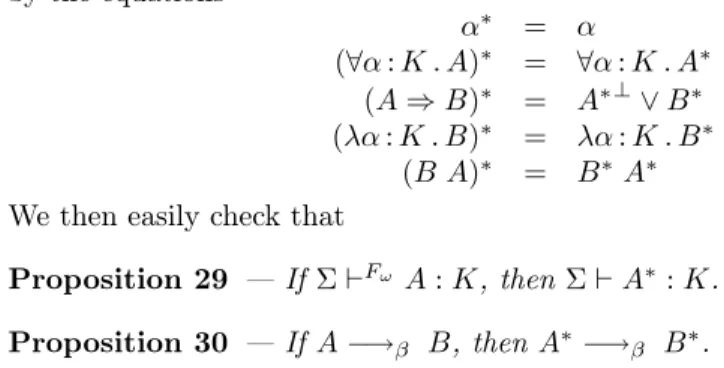
The translation proceeds as follows: each kind of Fω is translated as itself,
by the equations α∗ = α (∀α : K . A)∗ = ∀α : K . A∗ (A ⇒ B)∗ = A∗⊥∨ B∗ (λα : K . B)∗ = λα : K . B∗ (B A)∗ = B∗A∗
We then easily check that
Proposition 29 — If Σ ⊢Fω A : K, then Σ ⊢ A∗: K.
Proposition 30 — If A −→β B, then A∗−→β B∗.
We now translate proof-terms, adapting Prawitz’s translation of natural de-duction into sequent calculus, this time using Curry-style terms and programs, because without a typing derivation for the terms of Fω we lack some type
annotations to place in the encoding.
Definition 14 (Encoding of terms) The encoding u∗ of a term u of F ω is
defined by induction on u as described in Fig. 6. It relies on an auxiliary encoding that maps u to a program u∗
t and that is parameterised by a term t of
FC ω. x∗ = x λxA.u∗ = λxy.u∗ y Λα : K . u∗ = Λ_.u∗ u∗ = µy.u∗ y otherwise (u u′)∗ t = u∗hu′ ∗,ti (u A)∗t = u∗ h_,ti v∗ t = {v∗| t} otherwise
Figure 6: Encoding of terms
Remark 31 For a Curry-style term t and a Curry-style program p of FC ω, 1. If t −→FC ω t ′ then u∗ t −→FC ω u ∗ t′. 2. {u∗| t} −→∗ FC ω u ∗ t 3. u∗ t{x\u′∗ } −→∗FC ω u{x\u ′}∗ t{x\u′ ∗ } and u∗{x\u′∗ } −→∗ FC ω u{x\u ′}∗ .
The encoding of terms allows the simulation of reductions: Theorem 32 (Simulation of β for terms)
If u −→Fω u ′, then u∗ t −→ + FC ω u ′∗ t and u∗−→ + FC ω u ′∗.
Proof: By simultaneous induction on the derivation of the reduction step,
The translation preserves typing:
Theorem 33 (Preservation of typing for terms) 1. If Γ ⊢Fω
Σ u : A, then there exists a term t of system FωC (with type
anno-tations) such that ktk = u∗ and Γ∗ ⊢
Σ t : A.
2. If Γ ⊢Fω
Σ u : A and Γ∗, ∆ ⊢Σ t : A∗⊥, then there exists a program p of
system FC
ω (with type annotations) such that kpk = u∗ktkand Γ∗, ∆ ⊢Σp ⋄.
Proof: By induction on derivations, using Theorem 30 for the conversion rule. ✷ Since FC
ω is classical, we have a proof of the axiom of double negation
elim-ination:
Let ⊥ = ∀α : ⋆ . α (in Fω and FωC) and ⊤ = ∃α : ⋆ . α (in FωC), and let
DNE = ∀α : ⋆ . ((α ⇒ ⊥) ⇒ ⊥) ⇒ α in system Fω. We have
DNE∗= ∀α : ⋆ . ((α⊥∨ ⊥) ∧ ⊤) ∨ α. Let
C= Λα : ⋆ . λxByα⊥
.{x | hλx′αy′⊤.{x′| y}, hα⊥, yii}, where B = (α ∧ ⊤) ∨ ⊥.
We have
⊢ C : DNE∗
Hence, provable propositions of system Fω+ DNE become provable
propo-sitions of system FC ω:
Theorem 34 (Fω captures Fω+ DNE) For all derivable judgements of the
form
z : DNE, Γ ⊢Fω
Σ u : A
there exists a term t of system FC
ω (with type annotations) such that ktk = u∗
and we have
Γ∗ ⊢Σt{z\C} : A∗
Through the translation A 7→ A∗, system FC
ω appears as an extension of
system Fω+ DNE, and hence the consistency of FωC, proved in section 5.1,
implies that of Fω+ DNE.
We then set the following conjecture: Conjecture 35 (FC
ω is a conservative extension of Fω+ DNE)
There exists a mapping B of the upper layer of FC
ω into that of Fω such that:
1. If Σ ⊢FωA : ⋆, then there exist two terms u and u′ such that
⊢Fω
Σ u : A → B(A∗) and ⊢FΣω u′ : B(A∗) → A.
2. If Γ ⊢Σt : A then there exists a term u of Fω such that
B(Γ), z : DNE ⊢Σ u : B(A).
As mentioned in section 4, the mapping that forgets the information about duality is obviously not a good candidate to prove this conjecture, but ongoing work is about refining it for that purpose.
6
Conclusion
In this paper we have introduced a classical version of system Fω, called FωC.
Its upper layer is intuitionistic, its lower layer is classical, and both are strongly normalising.
We have adapted Tait and Girard’s reducibility methods for the two strong normalisation results, using orthogonality and, for the lower layer, Barbanera and Berardi’s symmetric candidates.
FωC thus provides an opportunity to tackle the two variants of the
reducibil-ity method, which we do in section 4, proving the conjecture set in [LM06] that orthogonality does not capture the fixpoint completion of the symmetric can-didates. It is worth noting that the counter-examples are not specific to FC
ω
at all. First, they hold in propositional logic (they do not involve polymor-phism or type constructors), and second they could easily be given for other symmetric calculi for classical logic such as the symmetric λ-calculus [BB96], the λµeµ-calculus [CH00] or the dual calculus [Wad03], as long as their untyped versions feature some infinite computations related to the λ-term ∆∆.
This point being made, it is clear that alternative proofs could have been given instead. For the upper layer we could simply have simulated the reduction in the simply-typed λ-calculus, forgetting all the information about duality (A and A⊥ would be mapped to the same term) which plays no computational role
in this layer.3
However, such an encoding, while preserving the notion of computation, loses all information about duality. This has two consequences:
• It cannot be used to establish a reflection between the upper layer of FC ω
and the simply-typed λ-calculus (or the upper layer of Fω).
• Since it loses all the logical meaning of type constructors, it cannot be used for a type-preserving encoding of FC
ω into e.g. Fω+DNE, which we
need to prove the conservativity conjecture (Conjecture 35 of section 5.2). Ongoing work is about refining this forgetful mapping by encoding in λ-terms the information about duality, i.e. some notion of “polarity”, in a way that is useful for the above two points.
For the lower layer we could try to adapt to Fω simpler proofs of strong
normalisation of symmetric and non-confluent calculi for classical logic, such as those of [DN05a] or [Dou06] which do not involve the fixpoint construction. We do not know whether these proofs break, for a typing system as strong as that of FωC. While we have seen that the fixpoint completion is not captured by
orthogonality, it would be interesting to see whether these simpler proofs are captured by it (although they are not expressed in the framework of reducibility to which orthogonality pertains).
3
For instance, α and α⊥would be mapped to the same term, A ∧ B and A ∨ B would both
be mapped to x∧∨A Band ∀α : K . B and ∃α : K . A would both be mapped to x∀∃λα.Afor
two particular variables x∧∨and x∀∃that are never bound because they represent the logical
References
[Bar84] H. P. Barendregt. The Lambda-Calculus, its syntax and semantics. Studies in Logic and the Foundation of Mathematics. Elsevier, 1984. Second edition.
[Bar91] H. P. Barendregt. Introduction to generalized type systems. J. Funct. Programming, 1(2):125–154, 1991.
[Bar92] H. P. Barendregt. Lambda calculi with types. In S. Abramsky, D. M. Gabby, and T. S. E. Maibaum, editors, Hand. Log. Comput. Sci., volume 2, chapter 2, pages 117–309. Oxford University Press, 1992.
[BB96] F. Barbanera and S. Berardi. A symmetric lambda-calculus for classi-cal program extraction. Inform. and Comput., 125(2):103–117, 1996. [BG01] H. Barendregt and H. Geuvers. Proof-assistants using dependent type systems. In J. A. Robinson and A. Voronkov, editors, Handbook of Automated Reasoning, pages 1149–1238. Elsevier and MIT Press, 2001.
[BHS97] G. Barthe, J. Hatcliff, and M. H. Sørensen. A notion of classical pure type system. In S. Brookes, M. Main, A. Melton, and M. Mislove, editors, Proc. of the 13th Annual Conf. on Math. Foundations of Programming Semantics, MFPS’97, volume 6 of ENTCS, pages 4– 59. Elsevier, 1997.
[CD78] M. Coppo and M. Dezani-Ciancaglini. A new type assignment for lambda-terms. Archive f. math. Logic u. Grundlagenforschung, 19:139–156, 1978.
[CH00] P.-L. Curien and H. Herbelin. The duality of computation. In Proc. of the 5th ACM SIGPLAN Int. Conf. on Functional Programming
(ICFP’00), pages 233–243. ACM Press, 2000.
[DGLL05] D. J. Dougherty, S. Ghilezan, P. Lescanne, and S. Likavec. Strong normalization of the dual classical sequent calculus. In G. Sutcliffe and A. Voronkov, editors, Proc. of the 12th Int. Conf. on Logic for Programming, Artificial Intelligence, and Reasoning (LPAR’05), vol-ume 3835 of LNCS, pages 169–183. Springer-Verlag, December 2005. [DN05a] R. David and K. Nour. Arithmetical proofs of strong normalization results for the symmetric λµ. In P. Urzyczyn, editor, Proc. of the 9th Int. Conf. on Typed Lambda Calculus and Applications (TLCA’05), volume 3461 of LNCS, pages 162–178. Springer-Verlag, April 2005. [DN05b] R. David and K. Nour. Why the usual candidates of reducibility do
and M. Zaionc, editors, Post-proc. of the 2nd Work. on Compu-tational Logic and Applications (CLA’04), volume 140 of ENTCS, pages 101–111. Elsevier, 2005.
[Dou06] D. Dougherty. Personal communication, August 2006.
[Gir72] J.-Y. Girard. Interprétation fonctionelle et élimination des coupures de l’arithmétique d’ordre supérieur. Thèse d’état, Université Paris 7, 1972.
[Gir87] J.-Y. Girard. Linear logic. Theoret. Comput. Sci., 50(1):1–101, 1987. [LM06] S. Lengrand and A. Miquel. A classical version of Fω. In S. van
Bakel and S. Berardi, editors, 1st Work. on Classical logic and Com-putation, July 2006.
[ML84] P. Martin-Löf. Intuitionistic Type Theory. Number 1 in Studies in Proof Theory, Lecture Notes. Bibliopolis, 1984.
[MV05] P. Melliès and J. Vouillon. Recursive polymorphic types and para-metricity in an operational framework. In P. Panangaden, editor, 20th Annual IEEE Symp. on Logic in Computer Science, pages 82– 91. IEEE Computer Society Press, June 2005.
[Par92] M. Parigot. λµ-calculus: An algorithmique interpretation of classical natural deduction. In A. Voronkov, editor, Proc. of the Int. Conf. on Logic Programming and Automated Reasoning (LPAR’92), volume 624 of LNCS, pages 190–201. Springer-Verlag, July 1992.
[Pol04] E. Polonovski. Strong normalization of lambda-mu-mu/tilde-calculus with explicit substitutions. In I. Walukiewicz, editor, Proc. of the 7th Int. Conf. on Foundations of Software Science and Computation Structures (FOSSACS’04), volume 2987 of LNCS, pages 423–437. Springer-Verlag, March 2004.
[Sel01] P. Selinger. Control categories and duality: on the categorical seman-tics of the λµ-calculus. Math. Structures in Comput. Sci., 11(2):207– 260, 2001.
[Ste00] C. A. Stewart. On the formulae-as-types correspondence for classical logic. PhD thesis, University of Oxford, 2000.
[Urb00] C. Urban. Classical Logic and Computation. PhD thesis, University of Cambridge, 2000.
[Wad03] P. Wadler. Call-by-value is dual to call-by-name. In Proc. of the 8th ACM SIGPLAN Int. Conf. on Functional programming (ICFP’03), volume 38(9), pages 189–201. ACM Press, September 2003.